Object Detection and Viewpoint Estimation with Auto-masking Neural Network Linjie Yang1 , Jianzhuang Liu1,3 , and Xiaoou Tang1,2 1
Department of Information Engineering, The Chinese University of Hong Kong 2 Shenzhen Key Lab of Computer Vision and Pattern Recognition Shenzhen Institutes of Advanced Technology, Chinese Academy of Sciences, China 3 Media Lab, Huawei Technologies Co. Ltd., China
[email protected],
[email protected],
[email protected]
Abstract. Simultaneously detecting an object and determining its pose has become a popular research topic in recent years. Due to the large variances of the object appearance in images, it is critical to capture the discriminative object parts that can provide key information about the object pose. Recent part-based models have obtained state-of-theart results for this task. However, such models either require manually defined object parts with heavy supervision or a complicated algorithm to find discriminative object parts. In this study, we have designed a novel deep architecture, called Auto-masking Neural Network (ANN), for object detection and viewpoint estimation. ANN can automatically learn to select the most discriminative object parts across different viewpoints from training images. We also propose a method of accurate continuous viewpoint estimation based on the output of ANN. Experimental results on related datasets show that ANN outperforms previous methods.
1
Introduction and Related Work
Category-level object detection has attracted a great deal of attentions in computer vision research. Aside from locating the object in an image, determining the pose of the object is also essential for practical tasks such as autonomous driving and robotic operation. Due to the large variance of the appearance of the object category, pose estimation remains a challenging task and a popular research topic in recent years. Part-based models have attracted a great deal of attention in object detection and viewpoint estimation. Recently proposed models include the star shape model [29], [24], [1], constellation model [7], [23], graphical model [25], and deformable part model (DPM) [6], [15], [19], [18]. The DPM in [6] initializes and learns object parts in a data-driven way without intensive human operations. Later, the DPM is extended to 3D DPM that can infer 3D positions of object parts [19], [18]. The integration of rendered images from CAD models provides viewpoint ground truth and more information about object appearance in training [14], [23].
2
Linjie Yang, Jianzhuang Liu, and Xiaoou Tang
To obtain viewpoint estimation, Pepik et al. [19] quantized the viewing circle into discrete bins and formulated the estimation as a multi-class classification problem. Later, they used an interpolation scheme from the predefined viewpoint bins to approximate the continuous viewpoint [18]. Other works to have targeted continuous viewpoint estimation are [28] and [30]. Teney et al. [28] fit a Gaussian distribution to the main peaks of voted scores to obtain an estimation of the continuous viewpoint, while Torki et al. [30] designed a regression function based on local features and their spatial arrangement. The part-based approaches have greatly improved the performance of object detection and viewpoint estimation. However, they require manually defined object parts with extensive human operation and intervention, or need to design a complicated algorithm to find object parts. Deep models have been successfully used recently in computer vision tasks such as pedestrian detection [21], face verification [9], face parsing [16], and classification [13], [22]. The research works of deep models focus on designing network structures [10], [2], [26] and feature learning algorithms [11], [27]. The convolutional neural network (CNN) [10] is one of the most popular deep models currently used to deal with computer vision problems [13], [21], [9], [26]. However, it still faces difficulties when applied to fine-grained tasks such as viewpoint estimation. The main reason is that although CNN is good at extracting global features, it does not emphasize local discriminative features which are critical for fine-grained tasks. Besides, the capability of CNN for continuous output tasks such as viewpoint estimation has rarely been explored, despite the fact that it succeeds in multi-class classification [9], [13]. In this paper, based on CNN, we propose a novel network structure, called Auto-masking Neural Network (ANN) for object detection and viewpoint estimation. ANN contains multiple CNNs and a mask layer that can select the most discriminative features from the input and pass them to the next level. It can also deal with multiple tasks such as object detection and viewpoint estimation simultaneously. Besides, a new method is presented to estimate the continuous viewpoint, which makes the estimation more accurate. Our experimental results show ANN outperforms the state-of-the-art algorithms.
2
Auto-masking Neural Network (ANN)
We have designed a deep neural network for the combined task of object detection and viewpoint estimation. Specifically, we have focused on a long-lasting and challenging task: car detection and viewpoint estimation. Our method is based on sliding windows, similar to the related works. At evaluation, it makes a prediction for each image patch. The structure of ANN is shown in Fig. 1, which has the following three parts: (i) the mask generator takes an image (patch) as input, and generates a mask; (ii) the mask operator does a mask operation between the input image and the mask, resulting in a masked image; and (iii) the target predictor outputs a detection label and a viewpoint from the masked image.
HOG ...,Ii ,... Image
CNN M
..., xj,...
CNNV
Mask ..., mi ,... Layer
3
...
Title Suppressed Due to Excessive Length
qV Masked Image
E ( p D , pV , q D , qV , m )
...,Iim,...
Mask Generator HOG Image ..., I ,... i
CNN D
qD Mask Operator
Target Predictor
Fig. 1. Structure of ANN.
ANN utilizes a mask layer and three CNNs to extract discriminative features from images. The three CNNs have different purposes. CN NM finds the positions of discriminative features from an input patch, while CN ND detects the object and CN NV estimates the viewpoint. The components of ANN are described in more detail in the following subsections.
2.1
Convolutional neural network (CNN)
CNNs have demonstrated their powerful capability in pedestrian detection [21], face verification [9], face alignment [26], and classification [13]. As an effective tool for learning global features, CNN’s capability to select discriminative features for fine-grained tasks such as continuous viewpoint estimation has rarely been explored in the literature. Fig. 2(a) shows the structure of CN NM , which contains one convolution layer followed by max pooling [10], and one locally connected layer followed by another max pooling. The purpose of the convolution layer is to discover positioninsensitive features in the image, while the purpose of the locally connected layer is to detect the position-sensitive patterns on top of the position-insensitive features. Fig. 2(b) shows the structure of CN ND (or CN NV ). The first four layers of CN ND (or CN NV ) have the same layer type as those of CN NM , but one more fully connected layer is appended in CN ND (or CN NV ). This fully connected layer is used to obtain the detection (or viewpoint estimation) result q D (or q V ). In our work, each image is rescaled to eight scales and image patches of size 200 × 200 are cropped using a sliding window. The input to ANN is a HOG image [3] with 23 × 23 blocks extracted from an image patch. The intensities of the HOG image are normalized to [0, 1]. The parameters (layer sizes) of the networks can be seen in Fig. 2.
4
Linjie Yang, Jianzhuang Liu, and Xiaoou Tang Input
Convolution
23
23 11 2
9
7
2
9
11
23
23
7
32 Max Pooling 32
36 Input
(a)
Convolution
23
23 11 2
3
7
2
3
7
11
23
23
32 Max Pooling 36
Locally Connected 11 5 2 2 5 11 32 Max Pooling 32
32
Fully Connected Locally Connected 11 5 2 2 5 11 32 Max Pooling 32
(b)
Fig. 2. (a) The structure of CN NM , (b) The structure of CN ND (or CN NV ). The sizes of the input, convolution, max pooling, and locally connected layers are illustrated by the cuboids with the numbers on their three dimensions. The local receptive fields of the neurons in the layers are illustrated by the small squares on the cuboids.
2.2
Mask layer
The mask layer is the key component of ANN. The whole network is trained automatically with the input HOG images and the target ground truth information (detection labels and viewpoints) through back-propagation. For each HOG image, ANN generates a specific mask, automatically finding important parts from the input and allowing only these parts to pass to the target predictor. The mask layer is fully-connected to the output of CN NM with bounded rectified linear neurons, the outputs of which are X mi = min{1, max{0, wij xj }}, i = 1, 2, ..., N, (1) j
where mi ∈ [0, 1] is the response of a node in the mask layer, xi is the response of a node in the output of CN NM , wij is the weight between nodes i and j of the two layers, and N is the size of the mask, which is 529 (23 × 23) in our setting (see Figs. 1 and 2). The mask operation is an element-wise minimum operation between the HOG image and the mask, resulting in the masked image with its intensities being Iim = min{mi , Ii }, i = 1, 2, ..., N,
(2)
where the mask and the HOG image are of the same size and Ii ∈ [0, 1] is the ith intensity of the HOG image. It is easy to see the masking effect: when mi = 0, the corresponding pixel i from the input is blocked by the mask; when mi ≥ Ii , it is passed completely (Iim = Ii ).
Title Suppressed Due to Excessive Length
5
Usually, only several key parts of an object in an image provide significant information for detection and viewpoint estimation. For example, the existence of a round wheel provides a strong indication that this image has a car that is viewed from the side. Therefore, we should enforce sparseness on the mask (i.e., mi close to 1 are sparse and most mi should be close to 0). Furthermore, considering that the features on the object should be more discriminative than those from the background, the positions with mi close to 1 should concentrate on the object. When a region larger than the object is cropped as the input (see Section 3 for the detail), the positions with mi close to 1 should form clusters on the object in the mask. Thus, considering mi as mass points on a plane, we minimize the following moment of inertia of mi in order to satisfy the sparseness and clustering requirements, X Esc = mi ri2 , (3) i
where ri is the distance from pixel i to the center of the mass of mi . Figs. 5 and 6 in the section of experimental results provide some examples of the masks superimposed on the corresponding images. We can see that the masks are sparse and the positions (bright) with mi close to 1 form clusters on the object. 2.3
Target prediction
In the target predictor, two CNNs, CN ND and CN NV , are used for object detection and viewpoint estimation simultaneously. Since the two tasks are quite different and require different filters that aim at different features, we allow them to have separate CNNs but to share the same masked image as the input. Their outputs are both probability distributions, where CN ND produces two outputs (object or non-object) and CN NV has Nvp outputs. For discrete viewpoint estimation, the Nvp outputs of CN NV represent Nvp probabilities of viewpoints within Nvp bins uniformly located on the viewing circle. The centers of the bins 360 i, i = 0, 1, ..., Nvp − 1. are θi = N vp In training, the cost for one input patch is the sum of the cross-entropy errors of the two CNNs and the sparseness and clustering cost, E=−
1 X i=0
Nvp −1 D D pD i log qi − p1
X
pVi log qiV + λEsc ,
(4)
i=0
D where pD = (pD 0 , p1 ) is the ground truth probability distribution for detection D (p = (1, 0) for a negative sample and pD = (0, 1) for a positive sample), pV = (pV0 , pV1 , ..., pVNvp −1 ) is the ground truth probability distribution for viewpoint (only one component of pV is 1 and the others are 0), q D and q V are the corresponding estimates for detection and viewpoint, respectively, and λ is a weighting factor. Here, the cost for viewpoint estimation is meaningful only when the input is a positive sample, which is why the second term on the right-hand side of (4) is multiplied by pD 1 .
6
2.4
Linjie Yang, Jianzhuang Liu, and Xiaoou Tang
Discrete and continuous viewpoint estimation
The most straightforward way of ANN training for viewpoint estimation is to set one of the pV ’s components (say, pVj ) to 1 and the other components to 0, where θjV is the center of the jth bin within which the viewpoint of the training object is located. We refer to this training scheme as discrete viewpoint training. In testing, for a predicted positive sample, the estimated viewpoint is set to θi if the largest component of q V is qiV . However, from our experiments, we find that ANN trained this way does not generate sufficiently precise viewpoint estimation because a lot of the information is lost when each of the continuous viewpoints of the training objects is abruptly quantized to only one component of pV . Next, we present an interpolation method to handle this problem. Let the ground truth viewpoint be θ, which is located between two neighboring viewpoint bin centers θj and θj+1 . Then pVj (θ) =
θj+1 − θ , L
pVj+1 (θ) =
θ − θj , L
pVk (θ) = 0, k ∈ / {j, j + 1},
(5)
360 where L = N is the size of a bin, and pVj , pVj+1 , and pVk are the components vp V of p . In this method, although there are only two non-zero components pVj and pVj+1 in pV when θ ∈ (θj , θj+1 ), pVj and pVj+1 implicitly encode all possible continuous viewpoint angles in [θj , θj+1 ], because from (5) we can have θ = pVj θj + pVj+1 θj+1 ∈ [θj , θj+1 ]. We call the training with pV defined by (5) PNvp −1 V continuous viewpoint training. Since j=0 pj = 1, pV can still be considered as a probability distribution. Objects of the same kind usually have similar appearances when they are in close viewpoints. The similarity between two objects in viewpoints θa and θb can be defined as
s(θa , θb ) = max{0, 1 −
|θa − θb | }, θT
(6)
where θT is a threshold, which makes the similarity to be 0 when |θa − θb | ≥ θT . 360 If θT is set to the size of a bin N , then vp pVj (θ) = s(θ, θj ), j = 0, 1, ..., Nvp − 1.
(7)
This relation indicates that pVj (θ) can also be regarded as the similarity between two objects in viewpoints θ and θj , respectively. V In testing, with the output q V = (q0V , q1V , ..., qN ) of ANN, on the manivp −1 V V ∗ fold p (θ) defined by (5), we find a point p (θ ) closest to q V with the pseudodistance Kullback-Leibler divergence [12], and use θ∗ to be the estimated viewpoint; i.e., Nvp −1
θ∗ = argmin {DKL (pV (θ)||q V )} = argmin { θ
θ
X j=0
pVj (θ) log
pVj (θ) }. qjV
(8)
Title Suppressed Due to Excessive Length
7
Fig. 3. Four examples of the non-photorealistic images of size 200 × 200 rendered from different 3D models in different views.
To solve the problem (8), we can start by finding all the local optimal solutions θi∗ ∈ [θi , θi+1 ), i = 0, 1, ..., Nvp − 1, and then obtain the global optimal solution θ∗ =
argmin θi∗ ,0≤i≤Nvp −1
{DKL (pV (θi∗ )||q V )}.
(9)
For θ ∈ [θi , θi+1 ), the problem (8) becomes Nvp −1
θi∗ = argmin { θ∈[θi ,θi+1 )
X
pVj (θ) log
j=0
pVj (θ) } qjV
(10)
pV (θ) pVi (θ) + pVi+1 (θ) log i+1 } V V qi qi+1 θ θi+1 − θ θi+1 − θ θ − θi θ − θi log log V }. = argmin { + V L L Lq Lqi+1 θ i
= argmin {pVi (θ) log
By
d θi+1 −θ dθ ( L
log
θi+1 −θ LqiV
+
θ−θi L
log
θ−θi ) V Lqi+1
θi∗ = θi +
= 0, we have
V qi+1 L . V V qi + qi+1
(11)
V Since qiV , qi+1 ∈ [0, 1], it is easy to verify that θi∗ ∈ [θi , θi+1 ].
3
ANN Training and Testing
Previous approaches [19], [18], [14], [23] have used not only real images but also non-photorealistic images rendered from 3D CAD models for training. These rendered objects are with known viewpoints (ground truth) and provide more information about object appearances. In our work, we also use the rendering of 3D CAD models for ANN training. Note that, like previous studies, we have only considered the estimation of viewpoint in horizontal directions without considering object tilt angles. We collected 93 3D car models from the internet and render the non-photorealistic images according to [4]. These models cover a wide variety of cars, including
8
Linjie Yang, Jianzhuang Liu, and Xiaoou Tang
Foreground Box Background
Fig. 4. The foreground box and the background on an image patch of size 200 × 200. The center of the foreground box is also at the center of the image patch.
limousines, pickups, SUVs, and vans. Four examples are shown in Fig. 3. We choose a fixed camera-to-car distance to generate all the non-photorealistic images from the 3D models. Each 3D model results in 180 projections (images) with a viewpoint difference of 2◦ between two neighboring projections. Each projected car is located approximately at the center of the image whose size is 200 × 200. In order to cover more car appearances in training, each projected 2D car C is used to generate four more car images, as follows. (i) C is rotated by an angle that is a sample from the Gaussian distribution with zero mean and standard variance of 2◦ . (ii) The rotated C is resized with these four scales 0.9, 0.95, 1.05, and 1.1. All these rendered (synthetic) images are used as positive samples for training. The previous template-based object detection methods work with a set of sliding windows with different scales and aspect ratios [8]. The sliding windows of different aspect ratios are used to cover the large shape variations of the objects in images. For example, Gu et al. [8] used 4–16 aspect ratios in their experiments. To obtain training samples from real images, when moving a sliding window on an image, an image patch under the sliding window is regarded as a positive A1 , sample if a ratio T1 is larger than a threshold (say, 60%). T1 is defined by A 2 where A1 is the area of the overlapping part between the sliding window and the bounding box of the object, and A2 is the sum of the sliding window area and the bounding box area minus A1 . We design a different sliding window method to obtain positive and negative training samples from real images, where the sliding window is square with size 200 × 200. An image patch covered by the sliding window is partitioned into two parts, the foreground and the background. The foreground is a rectangular region in the image patch called the foreground box, as shown in Fig. 4. The center of the foreground box is located at the center of the image patch. For an image patch containing an object, the size and shape of the foreground box are determined by the viewpoint of the object, B(I) = fB (θ(I)),
(12)
where B(I) denotes the foreground box in the image patch I, θ(I) is the viewpoint of the object in I, and fB (θ) is a function producing the foreground box from the viewpoint θ. We derive fB (θ) as follows. After normalizing the bound-
Title Suppressed Due to Excessive Length
9
ing boxes of all the objects to the same size (i.e., the same area = length × height), the bounding boxes of the objects in the same viewpoint have similar aspect ratios. Then, the average of the bounding boxes of the objects in the same viewpoint θ is defined as fB (θ). For a training image patch containing an object in viewpoint θ, if a ratio T2 is larger than a threshold, then the patch is 3 regarded as a positive sample; otherwise a negative sample. T2 is defined by A A4 , where A3 is the area of the overlapping part between the foreground box and the bounding box of the object, and A4 is the sum of the foreground box area and the bounding box area minus A3 . In testing, if pD 1 ≥ 0.5 for an input image patch, then the patch is predicted as a positive sample. Suppose that the predicted viewpoint is θ for a positive sample; we then use the foreground box defined by fB (θ) to be the bounding box for this positive sample. Although this foreground box may just be an approximation to the real bounding box of the object, it does show very good detection performance in our experiments. Note that the mask generated by ANN cannot be directly used to infer the bounding box of the object in testing. The positions with mi close to 1 may exist in the background of the patch, and there are only several clusters with mi close to 1 on the object, which do not give enough information to cover the whole object and only the object. HOG feature [3] is able to bridge the representation gap between real images and non-photorealistic images [19]. We extract HOG features (also called HOG images in this paper) from both the real image patches and the synthetic image patches. All these patches are of size 200 × 200, but the size of the HOG images is 23 × 23. In order to cover the size variations of the objects in real images, each real image is rescaled to eight scales in training and testing. Compared with previous sliding window methods, ours does not need a set of sliding windows with different aspect ratios to accommodate different object shapes; instead, our sliding window has only one shape (square), as shown in Fig. 4, which greatly reduces the number of image patches sampled in training and testing. In addition, a positive image patch contains not only the object but also part of the background (see Fig. 4). Incorporating the background around the object can provides more cues for object detection, because objects and their backgrounds usually have certain patterns in the scenes. For example, cars mostly remain still or run on streets, and ships float on water.
4
Experimental Results
In this section, we evaluate our ANN model for car detection and viewpoint estimation, and compare it with several state-of-the-art methods in [19], [18], [28], and [30]. In [19], there are two models, DPM-VOC+VP and DPM-3D-Constraints. The former includes a distinct mixture component for each viewpoint bin, and the latter adds 3D constraints across viewpoints in the DPM model. In [18], the authors construct a 3D DPM model called 3D2 PM. The methods in [28] and [30] give continuous viewpoint estimation via regression. Through cross-
10
Linjie Yang, Jianzhuang Liu, and Xiaoou Tang
validation, the parameter λ in (4) is chosen to be 1E-6 for all the experiments. For the evaluation of the effectiveness of the mask layer, we design a baseline network called CNN-V&D as follows. From ANN, we remove the mask generator and mask operator, with the HOG images directly inputted into CN NV and CN ND , and obtain detection label and viewpoint estimation as output. In the following comparisons, all of the results, except those obtained by our models, come from [19], [18], [28], and [30]. We use the 3D Object Classes car dataset [20] and the EPFL car dataset [17] in our experiments because they provide ground truth for both detection and viewpoint estimation. We train the ANN model using not only the real images from these datasets, but also the synthetic images generated from the 3D models (note that [19] and [18] also use real and synthetic images to train their models). When ANN is trained and tested on one dataset, the training real images are only from this dataset. ANN takes less than 1 second to obtain the result of object detection and viewpoint estimation for one input image of size 300 × 400, on a PC with a NVIDIA GTX 670 GPU. 4.1
Detection and discrete viewpoint estimation
Discrete viewpoint estimation can be regarded as a multi-class classification problem. 3D Object Classes annotates only eight different viewpoint bins, while EPFL provides degree-level annotations. We follow the previous protocols and report results of Mean Precision of Pose Estimation (MPPE) [19], [18], which is the average classification accuracy of multiple classes. The detection performance is evaluated by the widely used criterion Average Precision (AP) established in the Pascal VOC challenge [5]. Table 1 shows the results of AP (for object detection) and MPPE (for viewpoint estimation) obtained by five models on the 3D Object Classes car dataset. 3D2 PM-D is a version of 3D2 PM for discrete viewpoint estimation. ANN-D and CNN-V&D-D are ANN and CNN-V&D trained with the discrete viewpoint training scheme (see Section 2.4), respectively. The studies in [28] and [30] only provide the results of continuous viewpoint estimation and are therefore not available for comparison here. From Table 1, we can see that on this dataset, except CNN-V&D-D, all the models work very well in terms of AP, but ANN-D and DPM-VOC+VP perform the best in both AP and MPPE. Unlike the 3D Object Classes car dataset that gives only eight coarse viewpoint bins, the EPFL car dataset allows much finer comparison in viewpoint estimation. Table 2 shows the comparison results between our work and [18] for 18 and 36 bins. Note that 36 bins are the finest viewpoint estimation in [18], and the work in [19] does not have experiment on this dataset. In Table 2, 3D2 PMC Lin and 3D2 PM-C Exp are two versions of 3D2 PM targeting at continuous viewpoint estimation through linear and exponential combinations of the output scores in the discrete viewpoint bins, respectively. ANN-C and CNN-V&D-C are ANN and CNN-V&D trained with the continuous viewpoint training scheme (see Section 2.4) and evaluated in discrete viewpoints, respectively.
Title Suppressed Due to Excessive Length
11
Table 2 shows that the performances of ANN-C and the previous sate-ofthe-art method 3D2 PM-D are similar for 18 bins, but ANN-C obtains the best results for 36 bins in both detection and viewpoint estimation. It has significant improvement over the models in [18] in fine viewpoint estimation. Our continuous viewpoint estimation model (ANN-C) performs better than the discrete viewpoint estimation model (ANN-D) both for 18 bins and 36 bins. ANN outperforms the baseline model CNN-V&D with a large margin both in discrete viewpoint training scheme and in continuous viewpoint training scheme, which shows the effectiveness of the mask layer. Table 1. AP (for object detection) and MPPE (for viewpoint estimation) obtained by five models on the 3D Object Classes car dataset. AP / MPPE AP / MPPE DPM-3D-Constraints [19] 99.7 / 96.3 DPM-VOC+VP [19] 99.9 / 97.9 3D2 PM-D [18] 99.6 / 95.8 CNN-V&D-D 95.8 / 87.7 ANN-D 99.9 / 97.9
Table 2. AP / MPPE obtained by seven models on the EPFL car dataset. AP / MPPE AP / MPPE 18 bins 36 bins 18 bins 36 bins 3D2 PM-D [18] 99.2 / 71.8 99.3 / 45.8 CNN-V&D-D 96.6 / 62.5 97.0 / 46.4 3D2 PM-C Lin [18] 99.3 / 71.2 99.2 / 52.1 CNN-V&D-C 95.9 / 63.8 95.3 / 46.1 3D2 PM-C Exp [18] 99.2 / 70.5 99.5 / 53.5 ANN-D 99.2 / 70.5 99.9 / 53.1 ANN-C 99.6 / 71.4 99.9 / 58.1
4.2
Continuous viewpoint estimation
This section evaluates our model for continuous viewpoint estimation. Since the EPFL car dataset provides degree-level annotations, it is suitable for this experiment. Two measures are used for the evaluation: Median Angular Error (MAE) and Mean Angular Error (MnAE). Table 3 shows the results obtained by six models that can be used for continuous viewpoint estimation. The authors of [18] do not provide MnAE results. The models in [28] and [30] estimate viewpoints without the need of the parameter of viewpoint bins, while 3D2 PM-C Lin, 3D2 PM-C Exp, CNN-V&D-C and ANN-C are related to this parameter. This table shows that ANN-C outperforms the other models greatly with the much smaller errors. ANN also outperforms CNN-V&D in this experiment. Note that the two datasets are saturated for detection by the state-of-the-art methods, but they are not for viewpoint estimation, especially the EPFL car
12
Linjie Yang, Jianzhuang Liu, and Xiaoou Tang
dataset. For example, under 36 bins, the best MPPE and MnAE are only 58.1 and 27.6, respectively, which show that there are still large gaps for improvement. Table 3. MAE / MnAE obtained by different models on the EPFL car dataset. MAE / MnAE MAE / MnAE 18 bins 36 bins 18 bins 36 bins [28] 5.8 / 39.0 3D2 PM-C Lin [18] 5.6 / 4.7 / [30] 11.3 / 34.0 3D2 PM-C Exp [18] 6.9 / 4.7 / CNN-V&D-C 4.8 / 30.8 4.9 / 32.5 ANN-C 3.3 / 24.1 3.3 / 27.6
4.3
Mask layer
The mask layer plays a significant role for ANN to be the state of the art. It acts as a feature selector and finds the discriminative features for the object of interest to pass to the next stage of ANN. In Fig. 5 and Fig. 6, we superimpose some masks obtained by ANN on their corresponding positive testing samples. The bright parts on the images indicate the large responses of the masks. From our experiments, we have made the following observations. (i) Most large responses on the mask appear on or close to the car, meaning that the mask layer discriminates the car from the background in the image and prefers the features extracted from the car. Besides, the large responses in a mask are sparse and form clusters. (ii) For cars in similar viewpoints, the mask layer generates similar masks, which indicates that ANN can find similar patterns across similar viewpoints. This is true even for the images of cars of different kinds. Fig. 6 shows six different cars each in two views. The masks in the first row (viewpoint 1) are similar, and the masks in the second row (viewpoint 2) are also similar. (iii) Some car parts, such as the wheels, always have large responses on the mask. Wheels have similar shapes in different cars. Their appearances are also a strong indicator of the viewpoint of a car. For example, wheels are round in the side view and oval in the near-front and near-rear view of a car. ANN can capture the parts with discriminative features for the tasks of detection and viewpoint estimation. In Fig. 7, we examine the mask’s responses on negative samples. Note that a car or part of it can be in a negative sample if the overlapping between the bounding box of the car and the foreground box of the image patch is not large enough. The distributions of the large responses of these masks are clearly different from those in Figs. 5 and 6. These different distributions between positive and negative samples greatly benefit object detection and viewpoint estimation. All the above experiments and observations indicate that ANN is effective in dealing with the combined task, object detection and viewpoint estimation. The mask layer in ANN bridges CN NM with CN ND and CN NV , and plays an important role for feature extraction. We believe that the structure of ANN
Title Suppressed Due to Excessive Length
13
Fig. 5. Some positive sample images of the 11th car in the EPFL car dataset superimposed with their corresponding masks.
Fig. 6. Six different cars each in two views superimposed with their corresponding masks.
Fig. 7. Some negative samples from the EPFL car dataset superimposed with their corresponding masks.
14
Linjie Yang, Jianzhuang Liu, and Xiaoou Tang
can also be successfully applied to the detection and/or viewpoint estimation of other object categories.
5
Conclusion
We have proposed a deep model, known as ANN, for object detection and viewpoint estimation. ANN automatically learns to select the most discriminative object parts from training images without human interaction. Despite the simple procedures of ANN training and testing, it achieves the best performance among the state-of-the-art models. The experiments and observations on the masks produced by ANN show its effectiveness to capture the discriminative features from the input for the combined task. We believe that our model can be applied to many other object categories, especially those with relatively rigid objects such as bicycles, chairs, motorcycles, and ships, because compared with cars, they have similar appearance variations in different viewpoints, which is our future work. We also plan to apply ANN to other vision tasks such as object segmentation, classification, and detection.
Acknowledgements This work was supported by a grant from Guangdong Innovative Research Team Program (No. 201001D0104648280).
References 1. Arie-Nachimson, M., Basri, R.: Constructing implicit 3d shape models for pose estimation. In: ICCV (2009) 2. Ciresan, D., Meier, U., Schmidhuber, J.: Multi-column deep neural networks for image classification. In: CVPR (2012) 3. Dalal, N., Triggs, B.: Histograms of oriented gradients for human detection. In: CVPR (2005) 4. DeCarlo, D., Finkelstein, A., Rusinkiewicz, S., Santella, A.: Suggestive contours for conveying shape. In: SIGGRAPH (2003) 5. Everingham, M., Van Gool, L., Williams, C.K.I., Winn, J., Zisserman, A.: The PASCAL Visual Object Classes Challenge 2007 (VOC2007) Results. http://www.pascal-network.org/challenges/VOC/voc2007/workshop/index.html 6. Felzenszwalb, P.F., Girshick, R.B., McAllester, D., Ramanan, D.: Object detection with discriminatively trained part-based models. T-PAMI 32(9), 1627–1645 (2010) 7. Fergus, R., Perona, P., Zisserman, A.: Object class recognition by unsupervised scale-invariant learning. In: CVPR (2003) 8. Gu, C., Ren, X.: Discriminative mixture-of-templates for viewpoint classification. In: ECCV (2010) 9. Huang, G.B., Lee, H., Learned-Miller, E.: Learning hierarchical representations for face verification with convolutional deep belief networks. In: CVPR (2012) 10. Jarrett, K., Kavukcuoglu, K., Ranzato, M., LeCun, Y.: What is the best multistage architecture for object recognition? In: ICCV (2009)
Title Suppressed Due to Excessive Length
15
11. Kavukcuoglu, K., Sermanet, P., Boureau, Y.L., Gregor, K., Mathieu, M., Cun, Y.L.: Learning convolutional feature hierarchies for visual recognition. In: NIPS (2010) 12. Kullback, S., Leibler, R.A.: On information and sufficiency. The Annals of Mathematical Statistics 22(1), 79–86 (1951) 13. Lee, H., Grosse, R., Ranganath, R., Ng, A.Y.: Convolutional deep belief networks for scalable unsupervised learning of hierarchical representations. In: ICML (2009) 14. Liebelt, J., Schmid, C., Schertler, K.: Viewpoint-independent object class detection using 3d feature maps. In: CVPR (2008) 15. Lopez-Sastre, R.J., Tuytelaars, T., Savarese, S.: Deformable part models revisited: A performance evaluation for object category pose estimation. In: ICCV Workshops (2011) 16. Luo, P., Wang, X., Tang, X.: Hierarchical face parsing via deep learning. In: CVPR (2012) 17. Ozuysal, M., Lepetit, V., Fua, P.: Pose estimation for category specific multiview object localization. In: CVPR (2009) 18. Pepik, B., Gehler, P., Stark, M., Schiele, B.: 3d2 pm - 3d deformable part models. In: ECCV (2012) 19. Pepik, B., Stark, M., Gehler, P., Schiele, B.: Teaching 3d geometry to deformable part models. In: CVPR (2012) 20. Savarese, S., Fei-Fei, L.: 3d generic object categorization, localization and pose estimation. In: ICCV (2007) 21. Sermanet, P., Kavukcuoglu, K., Chintala, S., LeCun, Y.: Pedestrian detection with unsupervised multi-stage feature learning. In: CVPR (2013) 22. Sohn, K., Zhou, G., Lee, C., Lee, H.: Learning and selecting features jointly with point-wise gated Boltzmann machines. In: ICML (2013) 23. Stark, M., Goesele, M., Schiele, B.: Back to the future: Learning shape models from 3d cad data. In: BMVC (2010) 24. Su, H., Sun, M., Fei-Fei, L., Savarese, S.: Learning a dense multi-view representation for detection, viewpoint classification and synthesis of object categories. In: ICCV (2009) 25. Sudderth, E.B., Torralba, A., Freeman, W.T., Willsky, A.S.: Learning hierarchical models of scenes, objects, and parts. In: ICCV (2005) 26. Sun, Y., Wang, X., Tang, X.: Deep convolutional network cascade for facial point detection. In: CVPR (2013) 27. Taylor, G.W., Fergus, R., LeCun, Y., Bregler, C.: Convolutional learning of spatiotemporal features. In: ECCV (2010) 28. Teney, D., Piater, J.: Continuous pose estimation in 2d images at instance and category levels. In: Comp. and Rob. Vis (2013) 29. Thomas, A., Ferrar, V., Leibe, B., Tuytelaars, T., Schiel, B., Van Gool, L.: Towards multi-view object class detection. In: CVPR (2006) 30. Torki, M., Elgammal, A.: Regression from local features for viewpoint and pose estimation. In: ICCV (2011)