IEEE TRANSACTIONS ON COMPUTERS, VOL. C-18, NO. 12, DECEMBER 1969
1098
An
Algorithm
Decomposition Network Constraints for NAND
EDWARD S. DAVIDSON, Abstract-A branch-and-bound algorithm is presented for the synthesis of multioutput, multilevel, cycle-free NAND networks to realize an arbitrary given set of partially or completely specified combinational switching functions. In a programmed version of the algorithm, fan-in, fan-out, and level constraints may be specified. Cost may be specified as a nonnegative integer linear combination of gates and gate inputs. Further constraints and cost criteria are compatible with the algorithm. A first solution is constructed by a sequence of local decisions, and backtracking is executed to find improved solutions and to prove the optimality of the final solution. The completeness, consistency, and finite convergence of the algorithm are proven. Representative results from the computer program implementation of the algorithm are presented. Index Terms-Branch-and-bound algorithm, circuit constraints, combinational logic synthesis, decomposition, logic design automa-
tion, NAND synthesis.
I. PROBLEM DESCRIPTION AND THE BRANCH-AND-BOUND APPROACH C URRENT TRENDS in circuit fabrication toward large-scale integrated circuitry have greatly increased the need for an effective algorithmic approach to NAND network design. The NAND function is as basic to logic design, by virtue of its completeness, as it is to circuit fabrication, by virtue of its direct relation to the simplest of circuits. It is not unlikely that more complex logic functions used as "gates" by the logic designer -would be built up from NAND gates by the circuit designer at the most basic level. Within an LSI slice, one can thus expect an array of NAND gates and simple flip-flops. It is the contention of the author that in such a situation substantially more effective algorithms can be obtained using only NAND gates for atomic combinational logic modules than by using a larger and more complex collection of functions and their "gates" [3], [4]. The apparently nonintuitive nature of NAND logic design to the human designer makes an algorithmic approach to design imperative. In a complete logic design automation system, the specifications of a digital logic system accepted as input
would be partitioned into subsystem specifications of the logical complexity of single LSI slices. Within each slice, a state assignment problem would be solved. The subsystem specification would thereby be reduced to a Manuscript received November 22, 1968. This work was supported in part by the National Science Foundation under Grant GK-1663, and by the Office of Naval Research under Grant NONR225-83. The author was with the Coordinated Science Laboratory, University of Illinois, Urbana, Ill. He is now with Stanford Electronics Laboratories, Stanford, Calif. 94305.
Under
MEMBER, IEEE
set of assigned flip-flops and a set of combinational logic functions: one function for each subsystem output and flip-flop lexcitation function. Input variables for these functions are subsystem inputs and flip-flop outputs. An algorithm such as the one proposed here would then be executed to decompose each set of combinational functions to a set of NAND functions, i.e., to generate a NAND network to realize the undecomposed set of functions at its outputs. This task is referred to as NAND decomposition." Following NAND decomposition, other algorithms would be executed for flip-flop and NAND gate placement and routing of the interconnections between them. In the integrated circuit environment, network constraints will play an ever increasing role with respect to cost criteria. In the future, one can expect formulation both of network constraints and of cost criteria which are unfamiliar at present. Thus, any proposed algorithm to be of lasting value must be compatible with such new developments as they arise. Fan-in, fan-out, and level constraints are implemented in the computer program of the algorithm proposed here. Positive integers may be given to limit fan-in for gates, fan-out for gates, fan-out for variables, and the number of levels in the solution network for each required function. Any nonnegative integer linear combination of gates and gate inputs may be specified as the cost function. Thus, for example, gates or gate inputs (interconnections) or their sum (terminal pads) could be specified as the cost function. Further constraints and cost criteria are compatible with the algorithm and may be added in a straightforward manner due to the branch-and-bound structure of the algorithm. The algorithm generates solution networks of very
general form. Multioutput, multilevel, cycle-free, non-
tree-type networks are provided which realize a given set of partially or completely specified functions of a given set of completely specified variables. Due to the
reduced importance of finding optimum solutions, the algorithm was designed to produce a "good" solution relatively quickly and then to produce successively lower cost solutions, if necessary, until an optimum solution is found. A branch-and-bound technique was developed for the algorithm because this technique is directly related to the above goal of fairly general solutions to a broadly based set of problems employing a potentially wide variety of constraints and cost criteria. Branch-and-
DAVIDSON: ALGORITHM FOR NAND DECOMPOSITION
bound algorithms were originally named and described by Little et al. to characterize their approach to the traveling salesman problem [13]. In branch-and-bound algorithms, each terminal node of a solution tree represents a class of feasible solutions to the problem. Collectively they represent the class of all feasible solutions. Infeasible solutions, those which violate constraints, are discarded from solution classes as they are recognized. The algorithm begins by assigning the class of all feasible solutions to a single node treated as the original tree. Branching is employed to replace a selected terminal node of the tree with a set of terminal nodes whose solution classes partition the class of solutions of the replaced terminal node. A cost bound is then assigned to each new terminal node. The cost bound associated with a node is a lower bound on the cost of any solution in the solution class of the node. If the class is empty, the bound is infinite. These cost bounds determine a desirability order among terminal nodes which is used in the later selection of nodes for branching. The algorithm halts when every terminal node either represents a complete solution which has been generated by the algorithm, or has a cost bound which equals or exceeds the cost of the last solution found. The present algorithm is organized to consider for selection for branching only those terminal nodes which were added by the previous branching step. A first solution can thus be found relatively quickly since a single path of the tree is pursued until a solution is generated. After a solution is found, or if the terminal nodes considered have excessive cost bounds, backtracking [6] through the solution tree is employed to select the next terminal node. When no terminal node can be selected by backtracking, either the optimum solution has been found or no solution exists under the specified constraints. The generality of this approach to NAND network design is substantially greater than other known design algorithms. For example, Gimpel's extension to NAND networks of the 2-level, AND/OR, single-output QuineMcCluskey procedure imposes 3-level and single output restrictions [5]. Under these restrictions, however, Gimpel's algorithm has been programmed and is quite efficient. Some comparative results are given in Section V. Even in the more extensively explored AND/OR network design problem, approaches generalize only to the 2-level, multi-output case [1], [9] or the multilevel single-output case [12]. They generally remain incompatible with network constraint specification and some are restricted to a single cost function. Furthermore, in case an optimum solution cannot be obtained in the allotted time, no solution at all is obtained. Another class of algorithms based on functional decomposition techniques [10], [11], [15] is quite similar in philosophy if not in detail to the algorithm of this paper. The functional decomposition approach is in fact not restricted to NAND gates, but can accept a variety of modules. However, the efficiency of these algorithms appears to decrease rapidly as the number
1099
and complexity of the modules to be used increases [3], [4]. Comparative NAND network design results are discussed in Section V. II. PRELIMINARY DESCRIPTION AND NOTATION
Solution networks are generated by the algorithm, starting from the output gates of the network, each of which is to realize a required function. Uncovered true vectors of required functions are sequentially selected for covering. As vectors are covered, inputs are assigned to gates, new required functions and gates are added to the partial solution, and previously required functions become more completely defined. Vectors are selected according to a carefully developed set of heuristics based on difficulty of covering, so that only a small percent of the total number of vectors need be explicitly selected for covering. The particular cover to be implemented for a selected vector is chosen from a complete set of possible covers by another set of heuristics and is generally the cover with the lowest cost bound. A solution is obtained when all true vectors of required functions are covered. Although heuristics are employed by the algorithm, it is not a heuristic, i.e., nonoptimal, approach since backtracking is employed to insure that an optimum solution is always eventually found and proven optimum. When constraints are employed, possible covers which violate the constraints are simply not considered for implementation. Thus, any constraint for which such a violation test can be formulated is compatible with the algorithm. The particular cost bounding technique is also not basic to the algorithm. Cost criteria are compatible with the algorithm provided only that a lower bound can be calculated for the cost of solutions in a solution class. Naturally, possible constraints whose violation can be predicted early, and possible cost criteria yielding relatively tight bounding procedures would be preferred with respect to the efficiency of the algorithm. It should be reiterated that the algorithm deals intrinsically with multi-output, multilevel networks to realize partially or completely specified functions and that the algorithm provides a sequence of successively lower cost solutions, so that it may be halted before completion if fully optimum solutions are not required. The required combinational switching functions and the available input variables are represented by disjoint sets T and F of true and false input vectors, respectively. An input vector is an ordered sequence of zeros and ones; the value of the ith position of the sequence corresponds to the value of the ith input variable. These vectors in turn are represented by the decimal equivalent of the sequence of zeros and ones treated as a binary number. Thus, for example, the function g3 of Fig. 1 may be represented by true set T3 = { 1, 4, 5, 6, 71 and false set Fs = 10, 2, 3 1. Variable A, referred to as go, may likewise be represented by To = {1, 3, 5, 7 } and Fo = fO, 2, 4, 6}. The T and F sets are not simply complementary for partially specified functions whose un-
1100
IEEE TRANSACTIONS ON COMPUTERS, DECEMBER 1969
ified, initially required functions as well as initially required functions which can be realized with no gates, O 1 i.e., constant 0, constant 1, or a function identical to 0 O O 0 10 01 some variable, can be extracted prior to running the 1 1 0 1 algorithm. Second, minimum cost cycle-containing 1 1 0 1 combinational networks are a very restricted class and may possess undesirable properties [2]. The third Fig. 1. Truth table for function g3. Note: A =go; B-g1; C-g2. condition is achieved for NAND gate networks by the use of connectibility and by the solution of a covering specified vectors are neither in T nor in F. For consis- problem. tency then, both T and F sets are used throughout for Definition 2: A function or variable gI is connectible to definition of functions and variables. (is a possible input to) gate J if and only if FJC Tr (set The subscripts of T and F indicate the function or FJ is contained in TI). A function gi can be made convariable involved. Variables are numbered 0 through nectible to gate J if and only if F gTr, but F iF1 = q5. n -1 and functions n through m for an n variable probDefinition 3: A function or variable gi is a conceivable lem with m - n +1 required functions. The value of m input to gate J, IE CIj, if and only if gr is connectible increases as new required functions are added by the or may be made connectible to gate J, IdIIPj, and algorithm during the solution process. Required func- IEII Si. tions are at all times uniquely assigned to NAND gates Connectibility arises naturally from the nature of the of a partial solution so that function gj is assigned to NAND function. Consider, for example, gate J with gate J which is to realize gj at its output. Gates are inputs gt*, gj=A(gi, g12 * g18, gl2 y. g1,) thus likewise numbered from n to m. =grlVgi2 * * VgI If all functions are completely deEach gate of a partial solution is assigned a number fined, as in a network realization, TJ = F11UJF2 of inputs which may be variables or outputs of other UFI, and FJ= T1nT 26\ *.*OT18, which implies gates. Other interconnections, such as shorting two gate FjC TIk for k = 1, 2, * * * s. The conceivable inputs outputs together, are illegal. Thus, a variable or a gate include functions and variables which are connectible or output may be connected only to 0, 1, or more gate can be made connectible, and exclude functions and inputs. Gate J is said to be an immediate successor of gi, variables which are already inputs and those which i.e., JEISI, if and only if gate J has gi assigned as an would form cycles. input. Gate J is a successor of gi, JESI if there exists a Definition 4: A function or variable gI covers vector V , 1., gr8, such that of TJ if and only if JEISi and VE FI. Vector V of TJ series of functions grl, gi2, g. JEIS18, I.CIS18l, * *, I2EIS11, and I1CISi. I is is then type COV (covered). an immediate predecessor of gj, i.e., I&IPj, if and only Again, if all functions are completely defined, for gate if JC-ISI. I is a predecessor of gj, i.e., I(EP, if and only J inputs gl, gI2, * * *, gI8, TJ = F1UYFI2U . * F18. if JEES. A partial solution network may be completely Thus, the vectors of TJ must be covered by the vectors defined by the T and F sets of all functions and variables of F11, F12, * * , FI8. In a partial solution, vectors of T and the IP set of each gate. All other properties may be sets which are covered are of no further concern. derived from these. Definition 5: An uncovered vector V of TJ may Definition 1: A solution network of NAND gates for a become covered in one of a variety of ways: set of required functions is a well-formed network if and 1) by extending an input (immediate predecessor) only if: 1) each originally required function is assigned gI of gate J, i.e., adding V to FI provided V$E TI, to a unique gate in the network, 2) there are no cycles in an EXP (extend an immediate predecessor) the network, and 3) each required function is realized cover; by its assigned gate. 2) by adding J to ISI for a variable gr with gl E CIj It is assumed in the above definition that gates are and VC F1, a VAR (variable) cover; defined by stating their required functions and their 3) by adding J to IS, for a function gI with gl E CIj, input functions and variables, and that functions and gI connectible to gate J, and VE F1, an FCN variables are defined by their disjoint T and F sets. A (function) cover; cycle in a network is a sequence of gates such that each 4) by adding J to ISI and replacing TI by TIUF1 gate is an input to the next and the last gate is an input for function gI with gI E CiJ, gl not connectible a to the first. The first two conditions of the definition are to gate J, and VC FI, an MCF (make connectible imposed for the convenience of the algorithm, although a function) cover; in some cases it is profitable to assign two or more dis5) by adding J to ISI and V to FI for a function gI tinct partially specified initially required functions to with giECI1, gI connectible to gate J, VdF1, the same gate or to design cycle-containing combinaand VI TI, an EXF (extend a function) cover; tional networks. In defense of these restrictions it should be stated first that identical, completely spec6) by adding J to IS,-, V to Fi, and replacing Tr by C
B
o
o
A
0 O 1 10 1 1
3 0
.
.
,
-
.
.
DAVIDSON: ALGORITHM FOR NAND DECOMPOSITION
1101
TI'JFJ for a function gI with gi ECIJ, gI not tracking, the optimum solution has been found, or if no connectible to gate J, VEEFI, and VMET1, an solution has been found, no feasible solution exists. EXMCF (extend and make connectible a funcIII. EXPLANATION OF THE ALGORITHM FLOW CHARTS tion) cover; or 7) by creating a new required function gI, with In this section the algorithm is presented in detail. TI=FJ,Fi={V},andISs={J}, an NF (new Several refinements of the strategies for vector selecfunction) cover. tion, order of cover implementation, and backtracking can be presented only at such a detailed level. These These cover types are presented here in order by an refinements are the result of several months of careful a priori judgement of desirability, i.e., likelihood of pro- experimentation with the algorithm and are to a great ducing a minimum cost solution. This order has been extent responsible for the effectiveness of the algorithm. refined in the light of experimental results with the A comparative study of the results of each implemented strategy modification may be found in [2]. algorithm (see Section III). The algorithm begins with the initialization routine Definition 6: The type of a vector V of TJ is the type of its most desirable possible cover in the partial solu- of Fig. 3 which sets up the initial present partial solution at hand: COV, EXP, VAR, FCN, MCF, EXF, tion. A separate program has been implemented which EXMCF, or NF. The type of a function gj is the least converts variables and functions represented in sum-ofproducts form to the form required by the algorithm. desirable type among the types of vectors of TJ. Definition 7: Vector V of TJ is 1-COV if it is type The cost function is specified by two nonnegative EXP and there is a possible EXP cover by gI such that integers: input weight and output weight. The cost of a for all gK in IPI, VeTK and, if gI is not type COV or solution is then computed as: input weightXnumber of gate inputs +output weight X number of gates. Constraint EXP, then for all variables gK in ClI, VC TK. The type of function gJ is thus the least desirable information, e.g., fan-in, fan-out, and level limits, is cover type which is required in order to cover all vectors entered. The cost cutoff is a nonnegative integer which of TJ, assuming each vector is covered by its most desir- functions as a constraint on allowable solution cost. It able cover type. For example, T sets of EXP functions is updated at block 35, Fig. 2. The algorithm seeks contain only EXP and COV vectors. Their gates may only solutions with cost less than the cost cutoff. not require additional inputs. FCN functions would A and B are integers (B > A > 0) which are used in backrequire at least one additional input from some gate. tracking for reconstructing partial solutions (cf. blocks 1-COV vectors are a subclass of EXP vectors. They are 33, 40, and 41 of Fig. 2 and block 14 of Fig. 3). The loop of blocks 2 through 9 calculates the CI sets nearly covered and are not explicitly selected for coverby Definition 3. Any new functions added within this ing (see discussion of Theorem 2, Section IV). The algorithm begins by assigning each function to loop are not properly defined until block 10. They are be realized to a unique gate. NF vectors are removed by thus not added to CI sets within the loop. Since these adding the necessary new required functions and gates. new functions are not yet added to CI sets, a vector can A cost bound is then assigned this initial present partial apparently be type NF, but can have a cover by a solution. A vector, not type COV or 1-COV, is selected previously added new function (cf. block 4). In such a from some T set of the present partial solution. Each of case the test at block 6 will fail. F sets of new functions its possible covers is examined (branching). A tentative are reduced by block 6 to obtain either FLC TM or partial solution is constructed and a tentative cost bound FMC TL for each previously added new function gM. If is calculated for each possible cover (bounding). One of this relation can be achieved, then all the new functions these covers is then implemented by making its tentative added are necessary. If for some gL the relation cannot partial solution the present partial solution (and its be achieved, gL is not necessary and is abandoned. The tentative cost bound the cost bound). This process of test is arranged to add as many of the necessary new vector selection, cover evaluation, and cover implemen- functions as possible and to add no unnecessary new tation continues until either a solution is found (no functions. After the loop is executed for each originally required vector can be selected) or no acceptable solution can be derived from the present partial solution (no cover can function, blocks 10 and 11 properly incorporate the be implemented). When a solution is found, it is printed. new functions into the present partial solution. A In either case backtracking through the solution tree FCNTAG (function tag) item is added to the solution follows to find an unimplemented cover for a previously tree to record each new function added. A FCNTAG selected vector which might yield an "acceptable" solu- item for a new function gL includes the ISL element and tion, i.e., a feasible solution of cost lower than any solu- the FL element which together suffice to allow recontion yet found. The tentative partial solution of the struction of the partial solution. The loop of blocks 3 cover found by backtracking becomes the present par- through 9 is then executed for each new function. Some tial solution, and branching and bounding resume. of these may themselves possess NF vectors and require When no such cover can be found in the tree by back- additional new functions to be added. However, such
1102
IEEE TRANSACTIONS ON COMPUTERS, DECEMBER 1969
15a.
FAIL
Execute Algorithm Initializatio PASS
FAIL
1.Execute Constraint Routines I PASS
IF NO VECTOR SELECTED
16. Select VECTOR, an element from some
Ti
set not type COV or I-COV by:
goal 1: maximize difficulty of best cover goal 2: minimize number of possible covers
tree, Select first COVTAG item with lowest Effective Tentative Cost Bound from last group in tree satisfying: _i) Tentative Cost Bound < Cost Cutoff, and ii) Effective Tentative Cost Bound > Effective Tentative Cost Bound of CURTAG item (may be = if after CURTAG item in tree)
17. Push:
VECTAG item, Determine possible covers, gi, for VECTOR of Tj, Put
covering g 'Is in queue in order by cover
VAR, EXP, FCN, MCF, EXF, EXMCF
V
I F NONE I
18. Select a possible cover, gI, from queue
I
Cutoff = Solution Cost
36. Pop: REJTAG' items from end of
IF VECTOR SELECTED
type:
15. Print Solution, Set Cost
IF ONE
19. Calculate Tentative Partial Solution from Present Partial Solution: If FI S Tj: Tj = Tj UFI
NO SUCH ITEI ITEM NO GROUP IN GROUP SELECTED IN TREE 7. Print "LAST SOLPop:last 37. UTION PRINTED IS group from tree PTIMUM'"|
If J%ISI: CIK = CIKn([gKjUSJ) VKe([gI IUP) If FJ ¢ I: TI = TI UFJ If VECTOR
TK
=
CIK = CI n
Ci
==
OFI: FI= FIU
HALT
{VECTOR}, U IS,),
38. If CURTAG item Cover Type
TKU [VECTOR) VKe(IPI I VK3 ICCIK and CIifn[g4) VKeCII3
VAR, MCF,
VECTOR eFK, VECTOR
)
eFK
or
is EXP, 1 FCN, Push: REJTAG item , .~~~~~~~~~~~~~~~~~~~~~
39. Change CURTAG to COVTAG, Change selected COVTAG to CURTAG
40. Present Partial Solution = i) Solution B if number of CURTAG items > B, otherwise ii) Solution A if number of CURTAG items > A, otherwise iii) Solution 0
Find i) B+1
iii) 1
,
a
ii) A+1
at
or
VECTAG item in tree
Set VECTOR, J from VECTAG item
I
Set Cost Bound, I, Cover Type from next CURTAG item
Cost Cutoff
30. Add
as required functions the new functions as in FCNTAG items following CURTAG item
gL,
(and
Set
TL
in CURTAG item if Cover Type is = [gK: ISL element in
tree),
ISL
NF),
FK2 FL = [FL element in tree), CIL, Add gL to CI sets
=
*32. 13Calculate
Generate
31. If FI ¢:-T If JIS1: CIK
T =
If FJ ¢; TI J-
I
Tj
U
TI
TI
U
FjJ
VKe
([1)UPM)
OFI: FI = FI U [VECTOR) TK U (VECTOR) VKe (IPI U isI) Ci n {gI) VK3E ICCIK and VECTOR cFK
If VECTOR
TK
CIK
=
VKeCI)I3
NO
Inputs t.]~~~~~~~~~~~~
33. If number of CURTAG items in tree = A or B, Save Present Partial Solution
FI
CIjKl([g-JUSJ)
YES
ciII = CI IIn { fK I VECTOR Add J to IS1,I Delete I from CI
eFK
Fig. 2. Algorithm flow.
I~~~
1103
DAVIDSON: ALGORITHM FOR NAND DECOMPOSITION
Fig. 4. Typical constraint routine flow.
Fig. 3. Algorithm initialization routine.
additional new functions will be type VAR and cannot require further new functions. When all required functions are properly defined and no NF vectors are present, block 12 is executed. Inputs is a lower bound on the number of gate inputs of any complete solution derived from the present partial solution. It is sec equal to the number of elements in all IS sets plus 1 for each function which is not type COV or EXP. The cost bound is then input weightXinputs +output weightXnumber of gates in the present partial solution. If the cost bound is not less than the cost cutoff, no acceptable solution is obtainable and the algorithm halts. Otherwise, the present partial solution is saved for use in backtracking and block 15b of Fig. 2 is entered. A typical constraint routine flow is presented in Fig. 4. Constraint routines have been implemented for fanout, fan-in, and level constraints. Any combination of these constraints may be set for a particular prQblem
(cf. block 48). A fan-out limit for variables and a fanout limit for functions may be specified. These are upper bounds on the number of elements allowed in IS sets of variables and functions, respectively. The fan-in limit is an upper bound on the number elements in any IP set. Level limits may be specified for each function independently. The level limit for gj is an upper bound on the number of functions (not variables) which can ba listed in sequence ending with gj such that each function in the sequence, except for the first, is an element of the IS set of the previous function. At block 49 a check is made on the present partial solution for violation of the constraint under consideration. Some prediction of the inevitability of future violation is also included here. If constraint violation is found, the present partial solution is abandoned and backtracking is executed. Otherwise, any element I of a CGI set which would violate the constraint if it were added as input to gate J is deleted from CGj. For each such deletion a REJTA G' (reject tag for constraint purposes) item is added to the tree recording I and J for reconstruction of partial solutions. The loop of blocks 51 through 54 is then executed to
1104
add new functions required to remove any NF vectors created by deletions from CI sets. Here new functions are incorporated into the present partial solution as they arise rather than by the two step addition process of blocks 5, 6, 7, and 10. If there is a new function in ISK at block 52, an infinite string of new functions would be required since two new functions in succession are not sufficient due to the constraint. This condition is detected and backtracking is executed. At block 54 it is necessary to add only those CI set elements which would be considered legal by previously executed constraint routines. Again, if any would-be CI set element is illegal, a REJTAG' item is added to the tree. After no NF vectors are present, the cost bound is calculated for the modified present partial solution and a comparison to the cost cutoff is made. The constraint routines are called by block 15b of Fig. 2 each time a new present partial solution is constructed either by implementing a cover or by backtracking. Vector selection is accomplished by blocks 16 and 17, cover evaluation by blocks 18 to 28, cover selection and implementation by blocks 29 to 34, printing of solutions by block 35, and backtracking by blocks 36 to 47 and 32 to 33. Goal 1 of block 16 is realized by selecting the first function encountered which has the least desirable type of any function in the present solution. The function scan is from low- to high-numbered functions for all but VAR and EXP type functions. These are scanned from high to low. During early experimentation with the algorithm several types of VAR and EXP vectors were defined. "Bad" VAR vectors are least desirable among these, next are two types of "bad" EXP vectors, several types of "good" VAR vectors, and most desirable, "good" EXP vectors. It was only with such a refinement of desirability for vector selection that acceptable convergence of the algorithm was obtained. Selection of the vectors most difficult to cover tends both to increase the cost bound rapidly and to reduce the number of alternative covers eventually requiring examination. Goal 1 was temporized only when a potential redefinition of desirability in accordance with goal 1 led to first solutions of lower quality. Slower convergence from a good first solution usually implied less total running time than faster convergence from a bad first solution. Thus, for example, vectors which to be covered require the addition of their function to the IS set of some other function are selected in the order FCN, MCF, EXF, and EXMCF which is the reverse of least desirability order, but yields better first solutions. Realization of goal 2 directly reduces the number of alternatives at each branching and avoids some unnecessary decisions. Goal 2 is realized, once the type and function are selected, by selecting from the T set of the selected function the vector of the selected type with the fewest possible covers. The effectiveness of these strategies is evidenced by the 3- and 4-variable single function problems for which the average number of covers per se-
IEEE TRANSACTIONS ON COMPUTERS, DECEMBER 1969
lected vector was only 2.5, even though the minimum possible number is 2 (one for the selected cover type and one for the NF cover). In addition, the number of vector selections required to achieve a solution was on the order of the number of interconnections in the solution, which is but a small percent of the total number of vectors in the T sets of all gates. While the number of covers per vector selection tended to increase for larger problems, the number of vector selections required to characterize a complete solution continued to approximate the number of interconnections of the solution. A VECTAG (vector tag) item records J, the function selected, and VECTOR, the vector selected from TJ, in the tree at block 17. Possible covers are put in a queue in order by most desirability, except that VAR type covers are entered first. The ever-possible NF cover is not placed in the queue but is evaluated beginning at block 27. Block 19 begins to construct the tentative partial solution for each possible cover selected from the queue. TJ is enlarged if necessary to include FI, since gJ will be the NAND of gr and other inputs. Elements of CI sets which would form cycles due to the new interconnection of I to J are deleted. If gI must be made connectible to gate J, TI is enlarged to include FJ. If gI must be extended to cover VECTOR, VECTOR is added to FI. New elements of F sets must be added to the T sets of immediate predecessors to preserve connectibility, and to the T sets of immediate successors to preserve the NAND function. Finally, elements with VECTOR in their F sets are deleted from ClI and I is deleted from CI sets of functions with VECTOR in their F sets. This completes construction of the tentative partial solution except for the possibility of NF vectors being present. Any vectors which have become type NF due to the above manipulations are removed by adding the necessary new functions in blocks 20 through 23. This process is similar to that used in algorithm initialization (cf. Fig 3, blocks 4 through 11). When all NF vectors have been removed from all functions of the tentative partial solution, new functions included, the tentative cost bound is calculated. If the tentative cost bound is less than the cost cutoff and the removal of NF vectors did not violate constraints, the possible cover is recorded in the tree at block 26. A COVTAG (cover tag) item is PUSHed recording I, the cover type of the possible cover, and the tentative cost bound. Following this item a FCNTAG item is entered for each new function of the tentative partial solution. After each possible cover in the queue is evaluated, the NF cover is evaluated. The new function gI is set up by block 28. None of the operations of block 19 is required. NF vectors may only be found in gI itself at block 20. At block 29 one of the COVTAG items following the last VECTAG item must be selected for implementation. The tag of the selected item is changed to CUR-
DAVIDSON: ALGORITHM FOR NAND DECOMPOSITION
TAG to indicate that it is a currently implemented cover. The tree may thus begin with a string of FCNTAG items. The rest of the tree may be divided into groups of items each of which is begun by a VECTAG item (vector selection). Each group contains 0, 1, or more COVTAG items, and after implementation, 1 CURTAG item (one item per allowable cover). Each COVTAG or CURTAG item may be followed by 0, 1, or more FCNTAG items for new functions required by the cover. Each group (and the initial FCNTAG items if any) may end with a string of REJTAG items (introduced in backtracking) and REJTAG' items (introduced by constraint routines). The effective tentative cost bound is used to select the COVTAG item. The effective tentative cost bound equals the tentative cost bound except for VAR type covers for which it is reduced from the tentative cost bound by input weight plus output weight. The effective tentative cost bound thus favors the implementation of VAR type covers. It was found by experimentation that VAR covers, which should be implemented, frequently had a higher tentative cost bound than some other cover. The effective tentative cost bound was thus introduced and the quality of first solutions found by the algorithm was improved dramatically. In case of two or more COVTAG items with equal effective tentative cost bound, the first of these is selected. This strategy favors implementation of more desirable cover types first, and again favors VAR type covers (cf. order of evaluation of cover types at block 17). In the event no COVTAG item is present in the last group, all possible covers caused the NO exit to be used at block 25, and no acceptable cover exists for the last vector selected. The VECTAG item is POPped and backtracking is executed. If a COVTAG item is selected, block 30 begins construction of the tentative partial solution of the selected cover from the tree information. The required new functions, if any, are added. Block 31 for cover implementation essentially duplicates block 19 for cover evaluation. Much time could certainly be saved here and in backtracking by the use of a computer with enough fast storage to store and recover tentative partial solutions efficiently. In the absence of such storage capability, the Ath and Bth as well as the 0th (cf. blocks 1 and 14) present partial solutions are saved for use in reconstruction when backtracking. After the selected cover is implemented, the constraint routines are executed prior to selection of the next vector. If each vector in the T set of every required function or 1-COV, no vector can be selected at block 16, COV is a and complete solution has been obtained. This solution is printed at block 35. The cost cutoff is reduced and backtracking is executed to begin the search for a
lower cost solution.
Backtracking begins at block 36 at which a new CURTAG item for the last group of the tree is sought. The REJTAG' items which are associated with the
1105
present CURTAG item of the group are POPped. Condition i) insures that the potential CURTAG item is allowable; condition ii) insures that the potential CURTAG item has not been implemented previously. If no such item exists in the group, the entire group is POPped and the new last group of the tree is examined. If no groups remain in the tree, no improvement on the last solution found can be made. The last solution is then optimum and the program halts. If no solution has been found, then none exists within the constraints specified and with cost below the cost cutoff specified. If a new CURTAG item is found, block 38, in most cases, PUSHes a REJTAG (reject tag) item prohibiting the vector selected in the last group from also being covered by the cover of the previous CURTAG item. For a cover type in the previous CURTAG item of VAR, MCF, or FCN the previously covering gi is deleted from CIj, since the consequences of I in IPJ have just been investigated. The format of this REJTAG item is the same as for REJTAG' items. For cover type EXP, the selected vector is added to Tr, since the consequences of the vector being in FI have just been investigated. This type of REJTAG item records VECTOR and J. REJTAG items would be more complicated and less often used for cover types EXF, EXMCF, and NF and they are thus not employed. REJTAG items are POPped from the tree when their group is POPped at block 37. The introduction of REJTAG items allows the partitioning of solution classes by branching to be more nearly disjoint partitioning. The convergence of the algorithm was significantly improved by the introduction of REJTAG items. Block 40 determines the most recently saved partial solution which still obtains and uses it for beginning the reconstruction of the new present partial solution. Block 41 locates the first group in the tree not implemented in the saved partial solution. Blocks 42 through 45 implement the remaining groups of the tree. This process is similar to implementing a cover except for the possibility of REJTAG and REJTAG' items which are implemented by block 45. Any such items in the last group may raise the cost bound to or beyond the cost cutoff which necessitates the check at block 46. The YES exit rejects the new partial solution and returns to continue backtracking. Otherwise the new present partial solution is valid and blocks 32 and 33 are executed. The specified constraint routines, if any, are then executed prior to selection of the next vector.
IV. CONSISTENCY, COMPLETENESS, AND FINITE CONVERGENCE The theorems of this section are restatements of the theorems found in [2 ]. The proofs are omitted here, but may be found in the reference cited. Theorem 1: A cycle-free NAND network in which each initially required function is assigned a unique gate and in which each required function is covered and each
1106
IEEE TRANSACTIONS ON COMPUTERS, DECEMBER 1969
gate input is connectible is a well-formed network. Here, as previously, it is assumed that interconnections of a network are from a gate output to one or more gate inputs and never between gate outputs. Theorem 1 shows connectibility and covering to be at least as strong a condition as realizability of required functions. Definition 8: The completely specified function realized by gate J is gj* defined by TJ* and Fj*, where gj* = gi1Vgi2 V Vgin for gate J inputs gi1, gi2, * , gin. For variables, gj* and gj are the same. The above definition, of course, applies only to cyclefree networks. Definition 9: A vector V of TJ is Q- CO V (quasicovered) if and only if V is not type COV and possesses an EXP cover by a function gI with VCFI*. Theorem 2: For any well-formed network, all gate inputs are connectible and all vectors in the T sets of required functions are covered or quasi-covered. Thus, it appears that connectibility and covering together are a stronger condition than realizability. However, without modifying the interconnections of a network, unspecified vectors of required functions gj may be assigned as they are in gj*. After such an assignment, all vectors in the T sets of required functions will be covered. Connectibility and covering are thus only stronger than realizability with respect to the specification of vectors. They are equivalent conditions with respect to network topology. 1-COV vectors remaining in a complete solution network found by the algorithm are Q-COV. It is therefore not necessary to select 1-COV vectors for covering. Avoiding the selection of 1-COV vectors allows some unnecessary assignments of unspecified vectors to be likewise avoided. The concepts of 2-COV, 3-COV, etc., could be defined, but they would be progressively more complicated and difficult to use as well as less useful. Theorem 3: Given a set of variables and an originally required set of functions of those variables, a cost function and a cost cutoff, and a well-formed network with cost less than the cost cutoff, the algorithm will produce a well-formed network of cost equal to or lower than that of the given network. The proof of Theorem 3 develops a relation between the given network and the solution tree generated by the algorithm. The algorithm will depart from constructing a duplicate of the given network only to investigate seemingly more attractive alternatives. However, backtracking will always eventually return the algorithm to continuing construction of the duplicate network unless a solution of equal or lower cost is generated by the algorithm. Eventually the duplicate will be completed or a solution of equal or lower cost will be .
.
.
generated. 'Theorem 4: The algorithm will halt after a finite number of tree items have been generated. The proof of this theorem derives loose upper bounds on the number of VECTAG items in a tree at any one time (length of tree), on the number of COVTAG and
CURTAG items in any group (width of tree), and on the number of FCNTAG items after any COVTAG or CURTAG item or in the initial segment of the tree. The number of REJTAG and REJTAG' items is clearlyfinite since they delete elements from a finite number of finite CI sets and add elements to a finite number of bounded F sets. Thus, an upper bound is obtained on the total number of tree elements generated which includes any which may be generated but not PUSHed into the tree. It may be assumed that the real time between generation of tree items is finite. V. RESULTS In this section, representative solution networks and running times are presented as achieved by a programmed version of the algorithm. The program was written in ILLAR, an assembler with extensive macro capabilities developed at the Coordinated Science Laboratory. The program was executed on a CDC 1604 computer, which has a 6.4-,us (4.8 /is effective) memory cycle time and 32K words of 48 bit per word core memory. Approximately 5K of memory is reserved for storage of the solution tree, and 20K of memory for storage of the four partial solutions (the 0th, Ath, Bth, and present partial solutions). Solution networks are thereby restricted to no more than 86 gates for functions of no more than ten variables. The three-variable functions form an interesting class of functions for study. They are few and simple enough to consider all of them in a reasonable time, and they present design problems varied enough to test an algorithm effectively. There are 80 classes of threevariable functions under permutation of inputs. Of these, three trivial classes are not considered: constant 0, constant 1, and the class of functions identical to some input variable. A representative function was selected from each of the remaining 77 classes. These 77 functions were run in sequence as separate design problems under a variety of cost and constraint conditions. Spectra, pk'tting the number of functions against the number of required executions of backtracking, are shown in Fig. 5 and total run analysis statistics in Fig. 6. Time is recorded exclusive of input-output time. The cost function is presented as: (input weight, output
weight).
The first few runs are unconstrained and test various cost functions. Gate minimization (cost (0, 1)), run a), appears far preferable to the other cost functions used: (1, 10) minimizing gates, and secondarily, gate inputs, run b), and (1, 1) minimizing gates plus gate inputs, not shown. Under cost function (1, 1), the fourteenth function required over an hour and the run was stopped. Here, as in every other unconstrained problem studied, the running time of the algorithm increased significantly with the ratio of input weight to output weight. Also evident is that the time for a run of the 77 functions is largely consumed by very few of these functions. For run a), over half the total backtracking is consumed
DAVIDSON: ALGORITHM FOR NAND DECOMPOSITION
1107
found without difficulty, the "tree pruning" effect causes much faster convergence of the algorithm. HowA ~ 2rw0 IE9 ip ~~~~~~~~~ ever, if the first solution has a much more complex 50 100 200 300 400 500 ADDITIONAL FUNCTIONS FOR (b) solution tree or if it is found with great difficulty, the ---~~~~~~~~~~~~~~~~~~~ (a) 4 total time required by the algorithm may increase. i (b) --c--2 Level constraints tend to speed up the algorithm more wQyA. UI ;wi _ ,% than fan-in and fan-out constraints. 6 For functions as simple as the three-variable funcUl) z 5 0 tions, there is actually little difference in optimum solu4 3 tions as cost functions and constraints are changed as z 2 are here. Function 63 is most sensitive to the cost they 10 0 and constraint conditions used. It has four distinct 4 w optimum solutions under the six cost and constraint co conditions. These solutions are presented in Fig. 7. z For comparison's sake, Gimpel's IBM 7094 FORTRAN 6 6 program [5] required 59 seconds to solve the 80 func5,io 4 tions a 3-level constraint. The time required here under 2 -I -+. v .3 2C, is 99 for the 77 functions. A 4-variable, 3-level, seconds 2, single function problem taken from Gimpel's paper 10 required 9.8 seconds by his program as opposed to 4.9 6 f seconds required by this program. An exhaustive search procedure was used by Hellerman with an IBM 7090 10 20 30 40 50 NUMBER OF BACKTRACKS REQUIRED computer [8] to find optimum solution networks for the 80 functions of three variables with a (1, 10) cost funcFig. 5. Required backtracks spectra for 3-variable functions. tion and a set of priority rules for constraints. His approach required over 25 hours. a e b c d f The functional decomposition algorithm of Karp Cost (0, 1) (1, 10) (0, 1) (1, 1) (1, 0) (0, 1) et al. [11] was also programmed for an IBM 7090. The c 3 3 3 3 Levels oo c c cc 3 Fan-In x X of [11] for which optimality was proven are examples co cc c cc co 3 Fan-Out (Gates) 1246 6300 652 996 1166 721 Vectors Selected the 3-variable functions. It was stated that the majority Possible Covers Evaluated 2722 16068 1140 1878 2336 1281 980 4390 543 792 918 592 Covers Implemented was realized and proven optimum in nine secfunction 266 1910 114 274 338 169 Number of Backtracks 4:18 27:49 1:39 2:57 3:39 2:11 Time (Min: Sec) onds with NOR and 0 AND' building blocks. The longest realization and proof time for any 3-variable function Fig. 6. Run analysis: 3-variable functions. was ten minutes. The comparable figures for the algorithm of this paper using NAND (equivalently NOR) by 7 of the 77 functions; for run b), by 3 of the 77. building blocks are one second and one-half minute. When a level constraint of three levels is introduced, While a direct comparison of these times is improper a reduction in running time from four minutes and 18 due to the use of somewhat different gates and different seconds to one minute and 39 seconds occurs for cost computers, the substantial difference in times leads one function (0, 1), run c). This reduction is due to the "tree to speculate that the partitioning of solution classes by pruning" effect of the constraint. Furthermore, under functional decomposition alternatives as in [11] may the added constraint, the running time of the algorithm not be as efficient as by the vector selection technique varies comparatively little as the ratio of input weight of this paper. Several more difficult problems were to output weight is increased. Cost functions (1, 1), run presented in [11]. For these, first solutions of compad), and (1, 0), run e), require less than four minutes rable quality were found by the two algorithms, yet with a 3-level constraint, whereas previously, the more neither approach proved optimality in the allotted efficient cost function (1, 10), run b), required one-half time. A more fully discussed comparison of results may be found in [2]. hour and (1, 1) would have required many hours. For more complicated examples than these, no comAddition of a fan-in constraint of three and a fan-out limit for gates of three (with variables unrestricted in parisons with other methods are available. A fairly fan-out), run f), actually causes a slight increase in straightforward 6-function, 9-variable problem was running time with respect to a 3-level constraint alone, solved in three minutes and three seconds, yielding a with cost (0, 1), run c). Four of the functions possess no 14-gate, 31-input minimum gate solution. Yet some solution with the added constraint. These four are 4-variable, 1-function problems were found which could among the most time-consuming six functions. The not be solved optimally in ten minutes, although apother 73 functions yield the same solution networks as in run c). These results are fairly typical of the effects 1 The 0 AND is a no-cost AND function formed by connecting two of adding constraints. If reasonable first solutions are or more NOR gate outputs together. 50
40 30 20 10 6
-
I
It
-
0
11
50
0
1108
IEEE TRANSACTIONS ON COMPUTERS, DECEMBER 1969
VI. MODIFICATIONS
APPLICATIONS An algorithm which is quite general in its applicability
A5
B
B
~
~
~
~
(a)CostL=(, 1) or (1, 10), 6 C,7~~~~~~~~~ ate)3 15 inputs. gates,
A _g
B
~~
(b) Levels=3, cost=(O, 1) (1, 1), 7 gates, 17 inputs.
or
A
B
C
Fig.
r
(d) No
solution
possible
for
levels=3,3.fan-in=3, fan-out (gates)
A
=
(c) Levels=3, cost=(1, 0),
8
gates, 16 inputs.
Fig. 7.
Optimum solutions for function
parently good these
were
63:
ABVBCVACVAfiC.
were generally found. Most of easily solved with the addition of a
solutions
later
3-level constraint. The
running time of the algorithm
found to increase sharply as the number of variables increased, provided the most difficult functions of each number of variables are selected. This increase can be controlled somewhat by the proper use of constraints. The effect of adding required functions to a problem is not so straightforward. For example, the most difficult 3-variable functions were selected. A new problem was constructed from each of these by adding, as required functions, the output function of each gate in the optimum gate solution for the selected function. In each case, the algorithm immediately interconnected the gates, added input variables, and indicated that the optimum solution had been found. No other algorithm is known to the author which can actually decrease running time due to the addition of functions for simultaneous realization. There are, of course, multifunction problems which are more difficult to solve than their single functions alone. Such a case, for example, is the simultaneous realization of functions of completely different variables. As a final example, a 77-function, 3-variable problem was constructed from the 77 representative 3-variable functions used previously. An 82 gate first solution was found in 3 minutes and 50 seconds. After the NF vectors were removed, an 81-gate bound was calculated. In fact an 81-gate minimum gate solution is suggested by a careful examination of the 82-gate solution produced by the algorithm. Although backtracking through the solution tree in an attempt to remove the extra gate would probably be prohibitive, the easily attainable near optimum solution to a problem of this magnitude appears remarkable. was
AND
has been presented for NAND network synthesis. Its range of applicability and rate of convergence bear favorable comparison with other known algorithms which can be applied to NAND network synthesis. In this section several modifications of the basic approach are suggested. Their effect on the efficiency of the algorithm might be studied with reference to a particular
application. First, nonoptimal strategies should be considered. Such strategies would be particularly appealing as applied to problems large enough so that optimum
solutions would not likely be produced by the algorithm in the allotted time. Some measure, perhaps based on cover types of functions and cost bound, could be used to reject unappealing partial solutions while backtracking. Alternatively, the cost cutoff could be set to 80 or 90 percent of the cost of solutions found rather than 100 percent. This strategy would cause some tree pruning, yet would still guarantee optimality to within 20 or 10 percent. Some nonoptimum strategies could be extended to 2-pass optimum strategies, if necessary. Alternative optimum strategies form a second set of possible modifications for the algorithm. 1) Additional constraints and cost criteria can be added which might improve the efficiency of the
algorithm. 2) A more global covering problem could be formu-
lated. Rather than the covering of a single vector, the resolving of conflict situations could be investigated. Such an approach might yield a better cost bounding procedure and would be useful if excessive time were not required to find conflicts and determine their possible resolutions. 3) Unusual ways of proceeding from partial solutions to complete solutions could be incorporated in special situations. Such complete solutions could then be examined for areas of possible improvement. The algorithm could also be adapted for use as a solution improvement technique by introducing a CURTAG' tree item. This item would be used for the first implemented COVTAG item of a group. Condition ii) at block 36 would be waived when backtracking in a group with a CURTAG' item. Such a procedure would allow construction of a tree, or a final set of groups of a tree, to match a given or unusually generated solution. The search for improvement would begin by backtracking in the generated tree. CURTAG' items would revert to COVTAG' items indicating that they were previously implemented by an unusual selection procedure. Such a formulation would also allow for the application of one set of strategies when expecting a solution, seeking good solutions, and another set when expecting no solution, seeking fast rejection of bad solutions. 4) Certain vectors, particularly input vectors with a single 0, could be given special attention due to their form rather than their immediate covering potential.
DAVIDSON: ALGORITHM FOR NAND DECOMPOSITION
These vectors possess at most one variable cover. Since the number of these vectors is NUMVAR, rather than 2NUMVAR, and since they are expected to be influential, their selection and covering with some priority could help characterize a solution quickly. Also there is some evidence that type VAR vectors should be even more favored than at present. Very likely, a penalty should be associated with a cover which changes a function type from VAR, or a more desirable type, to a type less desirable than VAR. In another scheme, vectors whose selection caused abandonment of a partial solution and backtracking might be selected for covering with high priority if they are present in the new partial solution. Such a strategy might provide faster rejection of related sets of unproductive partial solutions. Each of the modifications in this second group seems appealing a priori. Each has an element of risk and could actually make the algorithm less efficient. However, they seem to the author to be worthy of further con-
sideration. Finally, more direct speedups of the algorithm can be undertaken. Use of a faster machine with more storage capability has an obvious advantage. More, if not all, tentative partial solutions could be stored and retrieved efficiently. Tentative partial solutions now implicitly constructed during cover evaluation could be explicitly constructed and then used directly for implementation at the next opportunity or after backtracking. Also, information about the tentative partial solution could be more easily extracted from such an explicit construction. Such information would be useful for constraint checks while evaluating covers, as well as for making a more careful decision on the order of cover implementation. This order could be made completely at will by simply pushing alternative covers into the tree in the desired order of implementation after all covers have been evaluated for a selected vector. Backtracking would then be appropriately modified. Naturally, a machine with some parallel processing capability might allow expansion of several paths of the solution tree concurrently. More information would then be present concerning areas of the tree to be further expanded immediately or temporarily abandoned when such a decision is to be made. Two applications of this algorithm come readily to mind. One is the application which motivated the development of the algorithm: the generation of NAND networks for a user faced with the problem of implementing sets of combinational switching functions with NAND gates. For this application, a method for partitioning larger design problems into subproblems would be highly desirable. Each subproblem could then be run until optimum solutions were provided. Output functions of gates of already realized subproblems could be introduced as "dependent" variables for the remaining subproblems. Such variables would not enlarge the T and F set size, nor would they be counted toward the 10-variable maximum. They would, however, be stored in memory and their number would be deducted from
1109
the 86-gate maximum. If necessary, after a solution to the partitioned problem has been found, improvements in the solution for the entire problem could be sought, provided the suggested modification for using the algorithm as an improvement technique were implemented. A second application of the algorithm is as a source of supply of NAND networks or optimum NAND networks, under constraints, for those who wish to study the properties of such networks. How should one partition a large problem? Are networks with few levels easier to diagnose? How much fan-in is useful for a 4-variable network? Do optimum networks for highly regular functions have highly regular interconnections? The list of such important, but as yet unanswered, questions is effectively infinite.
ACKNOWLEDGMENT The author is deeply indebted to Prof. G. Metze of the Coordinated Science Laboratory for his patient and enlightened guidance during the development of this algorithm. The assistance of C. Arnold of the Coordinated Science Laboratory, who is responsible for the programmed implementation of the algorithm, is gratefully acknowledged. The author also wishes to thank Prof. S. Muroga of the Department of Computer Sciences, University of Illinois, for the hours of illuminating discussions on integer linear programming and logic
design.
REFERENCES
[1] T. C. Bartee, "Computer design of multiple output logical networks," IRE Trans. Electronic Computers, vol. EC-10, pp. 21-30, March 1961. [21 E. S. Davidson, "An algorithm for NAND decomposition of combinational switching functions," Coordinated Science Laboratory, University of Illinois, Urbana, Rept. R-382, June 1968. [3] E. S. Davidson and G. Metze, "Comments on 'An algorithm for synthesis of multiple-output combinational logic,"' IEEE Trans. Computers (Short Notes), vol. C-17, pp. 1091-1092, November 1968. , "Module complexity and NAND network design algorithms," Proc. 6th Ann. Allerton Conf. on Circuit and System Theory, October 2-4, 1968. [5] J. F. Gimple, "The minimization of TANT networks," IEEE Trans. Electronic Computers, vol. EC-16, pp. 18-38, February
[4]
1967. [6] S. W. Golomb and L. D. Baumert, "Backtrack programming," J. ACM, vol. 12, pp. 516-524, October 1965. [7] B. B. Gordon, R. W. House, A. P. Lechler, L. D. Nelson, and T. Rado, "Simplification of the covering problem for multiple output logical networks," IEEE Trans. Electronic Computers, vol. EC-15, pp. 891-897, December 1966. [8] L. Hellerman, "A catalogue of three-variable Or-Invert and And-Invert logical circuits," IEEE Trans. Electronic Computers, vol. EC-12, pp. 198-223, June 1963. [9] R. W. House and T. Rado, "On a computer program for obtaining irreducible representations for two level multi-input-output logic systems," J. ACM, vol. 10, pp. 48-77, January 1963. [10] R. M. Karp, "Functional decomposition and switching circuit design," J. Soc. Ind. Appl. Math., vol. 11, pp. 291-335, June 1963. [11] R. M. Karp, F. E. McFarlin, J. P. Roth, and J. R. Wilts, "A computer program for the synthesis of combinational switching circuits," Proc. AIEE Symp. on Switching Circuit Theory and Logical Design, pp. 182-194, October 17-20, 1961. [12] E. L. Lawler, "An approach to multi-level Boolean minimization," J. ACM, vol. 11, pp. 283-295, July 1964. [13] J. D. C. Little, K. G. Murty, D. W. Sweeney, and C. Karel, "An algorithm for the traveling salesman problem," Operations Res., vol. 11, pp. 972-989, 1963. [14] S. Muroga, "Threshold logic," class notes, University of Illinois, Urbana, 1966. [15] P. R. Schneider and D. L. Dietmeyer, "An algorithm for synthesis of multiple-output combinational logic," IEEE Trans. Computers, vol. C-17, pp. 117-128, February 1968.