Lower Frame Rate Neural Network Acoustic Models Golan Pundak, Tara N. Sainath Google Inc., New York, NY, USA {golan, tsainath}@google.com
Abstract Recently neural network acoustic models trained with Connectionist Temporal Classification (CTC) were proposed as an alternative approach to conventional cross-entropy trained neural network acoustic models which output frame-level decisions every 10ms [1]. As opposed to conventional models, CTC learns an alignment jointly with the acoustic model, and outputs a blank symbol in addition to the regular acoustic state units. This allows the CTC model to run with a lower frame rate, outputting decisions every 30ms rather than 10ms as in conventional models, thus improving overall system speed. In this work, we explore how conventional models behave with lower frame rates. On a large vocabulary Voice Search task, we will show that with conventional models, we can slow the frame rate to 40ms while improving WER by 3% relative over a CTC-based model. Index Terms: speech recognition, recurrent neural networks, connectionist temporal classification.
1. Introduction Conventional hybrid neural network acoustic models output frame-level predictions for each content-dependent (CD)-state acoustic unit at every frame (i.e., 10ms) [2]. These CD-states are used as emission probabilities of a Hidden Markov Model (HMM). While the first generation of hybrid systems used Deep Neural Networks (DNNs) [3], more recently recurrent architectures, including Long Short Term Memory (LSTM) recurrent neural networks [4] and Convolutional Long Short Term Memory Deep Neural Networks (CLDNNs) [5] have shown additional improvements in hybrid systems. These models are typically trained using a frame-level cross-entropy criterion, followed by a sequence discriminative criterion [6]. One of the drawbacks of conventional models is that they require a framelevel alignment for cross-entropy training. To address the frame labeling issue, RNN-type architectures trained with a connectionist temporal classification (CTC) criterion were proposed [7]. CTC provides a mechanism to learn an acoustic model while mapping a sequence of input frames to a sequence of output labels. To allow for output sequences that are shorter than the input sequences, a blank output symbol is used in addition to the regular acoustic units in conventional models. In [1] it was shown that CTC-LSTM acoustic models outperform conventional LSTM models. To facilitate CTC training these CTC-LSTM models used one-state, context dependent phones (CD-Phones) [8]. One of the benefits of CTC with CD-Phones is that it allowed the model to output a symbol every 30ms, rather than the conventional 10ms. This lower frame rate reduced the length of both the input and output sequences, which reduces the computational cost during decoding and provided improvements in latency. In addition, at training time,
this setup reduces the number of possible different alignments of each output sequence which in turn reduces the difficulty of the task, yielding efficient training. While CTC does not require a pre-existing alignment, it also has a few drawbacks as well. First, [9] demonstrated that CTC models severly overfit to the training data, and could only match the performance of conventional models when trained with over 40,000 hours of data. Second, a consequence of using the CTC objective is that the time at which an output target is detected can be arbitrarily delayed after its corresponding input event. This means that a CTC-trained model is unable to produce accurate alignment of the input and output sequences. Therefore, additional latency might be introduced due to the delayed output. To overcome the latency problem, in [1] only alignments that do not deviate more than a 100ms from a given forced-alignment were used. This constraint was removed from the subsequent sequence training stage and the resulting models performed as well as unconstrained models, but resulted in a system with about 150ms of latency, compared to the conventional models which had only 50ms of latency. Third, while adding convolutional layers to the LSTM architecture was shown to help in [5] for conventional models, [1] did not find the additional layers to be helpful when trained with the CTC objective. The purpose of this paper is to explore how conventional LSTM-type models behave when trained with lower frame rates and CD phones. We will refer to this model as a lower frame rate (LFR) model. These models are trained using the standard cross-entropy and sequence training criteria. We note that although CTC models can be trained with lower frame rates as well, we use the term LFR to refer to conventional models, as these are the focus of investigation in this paper. On a large vocabulary Voice Search task, we will show that LSTM LFR models can match the performance of CTC models, both trained with 30ms frame rates. In addition, we address many of the concerns with CTC models addressed above. First, we will show that we can obtain an additional 3% relative improvement using a CLDNN with LFR compared to CTC. Second, with the LFR model we can increase the frame advance to 40ms with only an 80ms output delay, compared to the 30ms frame rate 150ms output delay with CTC. Finally, the LFR model is much more robust to smaller dataset sizes compared to CTC. The rest of the paper is organized as follows. In Section 2 we describe conventional and CTC training, as well as the LFR models explored in this work. In Sections 3 and 4 we discuss experiments and results, and finally conclude in Section 5.
2. Acoustic Modeling with LSTM RNNs In this section, we describe various approaches for acoustic modeling with neural networks. Once the acoustic unit is chosen (i.e., CD-states, CD-phones), training can use either hard
(Viterbi) or soft (Baum-welch) alignments. In addition, various objective functions can be used to train these models, including cross-entropy (CE), CTC and sequence training (ST). We will describe these different factors in the following section, including our proposed LFR model. For a more detailed summary of these different factors, we refer the reader to [9]. 2.1. Conventional Models Trained with Cross-Entropy Denote the input sequence for an utterance of length T as x = x1 , . . . , xT , where xt ∈ RN is a frame-level feature vector (i.e., log-mel feature), and w the output word word sequence. The acoustic likelihood can be written as follows, using the Viterbi approximation: p(x|w) =
T Y
2.1.2. LFR models Stateful, recurrent acoustic models are capable of processing more input before emitting a prediction, thus there is no need to assume signal stationarity. It follows that there is no need to break a phone into sub-units, and instead the HMM can use phones directly (e.g. CD-Phones [8]). These modifications allow us to remove the 10ms restriction, and in LFR modeling, we compute the output label lt at a lower frame rate, or equivalently, higher frame advance (i.e., 20ms, 30ms, etc.). While alternative front-ends are conceivable, in this work we use a typical 10ms log-mel frontend, but stack consecutive frames together to make up for the lower rate, and then subsample the frames to the desired frame rate, as in [4]. Soft-target label class posteriors are created by averaging across the 10ms posteriors in the desired frame rate window.
p(xt |lt )p(lt |lt−1 ),
t=1
Here l1 , . . . , lT is the label sequence computed by forced alignment of the utterance with the word sequence w, and is typically performed by a pre-existing model such as a GMM or neural network 1 . In hybrid decoding, the emission probabilty of the HMM is given as p(xt |lt ) = p(lt |xt )p(xt )/p(lt ), Here the label posterior is given by the output of a neural network acoustic model, and can be computed using using a context of L frames to the left and R frames to the right of the current frame, denoted as p(lt |xt ) ≈ p(lt |xt−L : xt+R ). This allows the neural network to incorporate acoustic context when making frame-level predictions for lt . The label prior p(lt ) is obtained by counting the label frequency produced from the forced alignment. The data likelihood p(xt ) does not depend on labels and thus can be ignored for training and decoding purposes [2]. Given input sequence x and corresponding frame level alignment l of equal size, the neural network acoustic model is first trained to maximize the CE loss on all acoustic frames, as follows |x| XX LCE = − log p(lt |xt ). (1) (x,l) t=1
Here p(l|x) is the label posterior after the softmax output layer of the neural network. A weakness of this criterion is timeindependent treatment of each label. This can be fixed with additional training using a seqeunce discriminative criterion, as discussed below. 2.1.1. Conventional modeling Most ASR systems make the assumption that on a 10ms time scale the speech signal can be approximated as a piecewisestationary process, giving rise to locally shift invariant representations produced by a frontend every 10ms (e.g. xt are logmel filterbanks). As phones emerge on longer time scales, each phone is typically broken into 3 piecewise-stationary models, where the corresponding HMM topology is a 3-state, left-toright model, with self loops. Stateless acoustic models (e.g. GMM, DNN) are trained to provide a distribution p(xt |st ) over the HMM states every 10ms thus matching the frontend frame rate. CE training is then carried out as described above with fixed alignments provided by a trained 10ms model. 1 It should be noted that while most conventional models do require a fixed alignment, there has been work with conventional models where the alignment is learned online [10]
2.2. Acoustic Models trained with CTC The connectionist temporal classification (CTC) [7] approach is a training criterion for sequential models such as RNNs, where the acoustic model is learned jointly with the label sequence. CTC models differ from conventional framewise models in two ways. First, CTC models introduce an additional blank label to relieve the network from making label predictions at a frame when it is uncertain. Second, the training criterion operates at a sequence level, and optimizes the log probability of state sequences, rather than the log likelihood of independent input frames as in Equation 1. The CTC loss function is defined as the sum of negative log probability of correct labelings for each training example: X LCT C = − lnp(z l |x) (2) (x,l)
where x is the input sequence of acoustic frames, l is the target label sequence (e.g. phonetic transcription for the utterance), z l is the lattice encoding all possible alignments of x with l which allows label repetitions possibly interleaved with blank labels. The probability for correct labelings p(z l |x) can be estimated using the following equation: XY t p(z l |x) = y πt (3) π∈z l
t
yst
Where is the softmax output at time t for symbol s, and π enumerates over all paths in z l . The tractable forward-backward algorithm is used to compute the summation (See [7] for more details). As seen in equation 3, the output labels are considered independent given the internal state of the network, which hinders the incorporation of language model information. This weakness can be alleviated with additional training using a seqeunce discriminative criterion. In this work, the label sequence we explore for CTC is the same one used for the conventional models, namly CD-phones. 2.3. Sequence Discriminative Training After CTC or CE training is done, typically the model is retrained using a sequence-level discriminative training criterion, which is more closely matched in objective function to the ASR WER objective [11]. In practice, ST has been shown to improve neural network models trained with either cross-entropy or CTC training [12, 13, 9]. In this paper, we explore training all of our models with the state-level minimum Bayes risk (sMBR) criterion [12].
3. Experimental setup 3.1. Neural Network Architecture The acoustic features used for all experiments are 80dimensional log-mel filterbank energies computed on 25ms window every 10 ms. At the current frame t, these features are stacked with l = 7 frames to the left and downsampled to the desired frame rate, to produce a 640-dimensional feature xt−l : xt . This is the same feature used for all NN experiments in this paper, and is similar to the features used in [4] Similar to [4], the LSTM models used in this work for CTC training consist of 5 LSTM layers, with 640 hidden units per layer and no projection layer. This amounts to ∼20M parameters. The CLDNN [5] models used for LFR-modeling have convolutional, LSTM and DNN layers. First, the 8 × 80 time×frequency log-mel feature is fed into a single convolutional layer with a filter size of 8 × 15 and 256 feature maps. After convolution, we use non-overlapping max pooling in frequency only with a window size of 6. The output of the convolution layer is passed to a linear bottleneck layer with 256 outputs, followed by 3 LSTM layers with 832 cells and a 512 unit projection layer. Finally, we pass the output of the LSTM to a fully connected ReLU layer with 1,024 hidden units. Again, to reduce the number of parameters, the softmax layer is factored into two with an intermediate 512-node linear low-rank layer [14]. The CLDNN model also has ∼20M parameters. All acoustic models have 9,287 CD-phone output targets [8]. 3.2. Training procedure The LFR models are initially trained with CE using asynchronous stochastic gradient descent (ASGD) optimization [15]. The models use an existing forced-alignment generated by an existing 10ms CD-state model. Features are extracted and stacked, and we keep every n-th feature-frame (e.g. n=3 for 30ms) and drop the rest. CTC models were trained using the same frontend configuration producing frames every 30ms. (see [1] for more details). For LFR models we map the CD-states to CD-Phones and subsample by averaging n 1hot target labels, producing soft targets. All LFR models are trained with a 1-state HMM. Models are then further trained sequence-discriminatively using sMBR with a setup similar to [6]. During training, recurrent networks are unrolled for 20 time steps for training with truncated back-propagation through time (BPTT) [16]. All results are reported after ST. In addition, the output state label is delayed by k frames, where k is chosen experimentally to strike a good tradeoff between accuracy and latency, as will be shown in the results.
overall SNR is between 5dB and 30dB. Samples of noise were taken from YouTube and daily life noisy environmental recordings. We use 20 different noise and reverberation conditions for each utterance. The full dataset consists of roughly 40,000 hrs, though only 2,000 unique label-alignments. Our evaluation set consists of a separate set of about 30,000 utterances (over 20 hours) with similar noise conditions to the training set.
4. Results 4.1. Factors in LFR Models First, we sweep different parameters in the CLDNN LFR models to understand their behavior. 4.1.1. Language Model Weight Whenever a new acoustic model is explored, language model weights are typically readjusted [4]. Typical viterbi decoders attempt to maximize the probability of emitting word sequence, w, given a sequence of acoustic observations, x: p(w|x) ∝ p(x|w)p(w)α
(4)
In this equation, α, the Language Model Weight (LMW), is a scaling factor which is introduced to compensate for the fact that acoustic scores are computed every frame while LM scores are applied every word. The LMW is important during decoding and for ST lattice generation. Since the number of frames per word increases with the frame rate, we expect that lower frame rates will require lower LMW. For each CE trained model, the LM weight which produces the lowest WER was determined by sweeping a range of possible values, as shown in Figure 1. As expected the optimal LMW was found nearly linearly proportional to the frame rate.
3.3. Decoding procedure All acoustic models are decoded with a single pass WFST-based decoder which uses a 100-million n-gram language model and a vocabulary larger than 5 million words. The decoder performings beam search and only keeps 7,000 active arcs at any point in time.
Figure 1: Word Error Rate (%) versus Language Model Weight for various frame durations. 4.1.2. Delayed Output
3.4. Data Sets For our experiments we use a mutli-style training procedure [17], where we first start with clean 3m utterances (about 2,000 hrs) which are anonymized and hand-transcribed voice search queries, and are representative of Google’s voice search traffic. Next, we create a noisier version by adding varying degrees of noise and reverberation at the utterance level, such that
The CTC models trained in [1] produce about 150ms of latency between input events and output symbol emission. For fair comparison, we trained LFR models with outputs delayed for a few frames to roughly match 150ms. As can be seen in table 1 WER decreases with lower frame rates up to 40ms, and then starts to increase. We will provide some intuition for this behavior in the next section.
Table 1: Word Error Rates (%) and Output Delays Model Output Delay WER (%) CTC-30ms 150ms 12.3 LFR-10ms 150ms 13.0 LFR-20ms 140ms 12.1 LFR-30ms 150ms 11.9 LFR-40ms 160ms 11.8 LFR-50ms 150ms 12.0 LFR-60ms 120ms 12.5 LFR-70ms 140ms 13.9
the alignment jointly with the labeling. Perhaps including a convolutional layer, which makes the CTC network have 6 layers, makes the optimization more difficult. Table 2: Models with and without convolution Model No Convolution With Convolution CTC 30ms 12.6 12.9 LFR 30ms 12.3 11.9 4.3. Shorter output delay
4.1.3. WER Analysis In order to gain some insight into the effect of lower frame rate, Figure 2 compares the insertions, deletions and substitution rate of the different LFR models. We first observe that the 10ms model suffer from high degree of insertions. This can be attributed to the 1-state HMM topology which forces minimal duration of 10ms per phone as opposed to the 30ms that is typically used with a 3-state HMM. On the other hand, the number of deletions increases as the frame rates increases above 40ms. To understand this phenomena better, we examined the distribution of phone duration, according to forced alignment and found that 10% of the phones have duration of 40ms or less. This means that for lower frame rates the more phones are likely to occupy the same frame. Since the decoder has to choose one of them, some deletions are expected. Another hypotheses we have for the degradation in WER when the frame rates are too long is that the 30ms model, for example, is trained on twice the number of frames as the 60ms model. Smaller amounts of training data can also lead to degradations in WER.
So far we have shown that LFR models can reduce the frame rate below 30ms with improved WER, and the same 150ms output label delay that CTC introduces (Table 1). In [1] it was found that below 150ms output label delay CTC model preformance degrades. We were curious to see if the same is true for CLDNN-LFR models. Table 3 shows that for conventional models we can reduce the output delay to 80ms, about half that in CTC, and still maintain roughly a 3% relative improvement over the CTC model. To summarize, we have found that the CLDNN LFR model offers an improvement in both accuracy and latency with respect to the LSTM CTC model. Table 3: Word Error Rates (%) and Output Delays Model Frame Duration Output Delay CD-Phone CTC 30ms 150ms CD-Phone CLDNN 40ms 0ms CD-Phone CLDNN 40ms 80ms CD-Phone CLDNN 40ms 160ms
WER 12.3 13.9 11.9 11.8
4.3.1. Training Data Finally, as noted in [4], CTC is very sensitive to the amount of training data used, since it must learn alignments. Therefore, we compared CTC vs. LFR performance as we vary the amount of training data. Table 4 shows how the conventional model degrades more gracefully than CTC, requiring about fourth of the data to reach the same performance. Table 4: Training with smaller amounts of data Training hrs CTC LFR 30ms 500 22.8 17.8 20.4 16.1 1000 2000 17.7 15.7
Figure 2: Word Error Rate (%) versus frame durations. 4.2. Comparison of LFR vs. CTC Models In this section, we compare LFR to CTC models. 4.2.1. Convolution Previous LSTM-CTC models did not show gains when combined with convolution. In this work we compared a conventional LSTM with a conventional CLDNN at lower frame rates. To match the number of parameters we added another LSTM layer to the non-convolutional model (totaling 4 layers), so both models have ∼20M parameters. As shown in Table 2, convolution gives about 0.5% improvement for the LFR model, while the CTC model seems to degrade with it. One hypothesis we have is that CTC models are difficult to train, as they must learn
5. Conclusions In this paper, we presented a CLDNN LFR model. We have shown that these models can achieve a 3% relative improvement over the CTC model with reduced latency and graceful degradation on smaller datasets.
6. Acknowledgements The authors would like to thank Michiel Bacchiani and Johan Schalkwyk for suggesting and supporting the research and Olivier Siohan and Hasim Sak for useful discussions.
7. References [1] A. Senior, H. Sak, F. de C. Quitry, T. N. Sainath, and K. Rao, “Acoustic modeling with CD-CTC-SMBR LSTM RNNs,” in Proc. ASRU, 2015. [2] H. Bourlard and N. Morgan, Connectionist speech recognition. Kluwer Academic Publishers, 1994. [3] G. Hinton, L. Deng, D. Yu, G. Dahl, A. Mohamed, N. Jaitly, A. Senior, V. Vanhoucke, P. Nguyen, T. N. Sainath, and B. Kingsbury, “Deep Neural Networks for Acoustic Modeling in Speech Recognition,” IEEE Signal Processing Magazine, vol. 29, no. 6, pp. 82–97, 2012. ˙ [4] H. Sak, A. Senior, K. Rao, O. Irsoy, A. Graves, F. Beaufays, and J. Schalkwyk, “Learning acoustic frame labeling for speech recognition with recurrent neural networks,” in Proc. ICASSP, 2015, pp. 4280–4284. [5] T. N. Sainath, O. Vinyals, A. Senior, and H. Sak, “Convolutional, long short-term memory, fully connected deep neural networks,” in Proc. ICASSP, 2015. [6] G. Heigold, E. McDermott, V. Vanhoucke, A. Senior, and M. Bacchiani, “Asynchronous stochastic optimization for sequence training of deep neural networks,” in Proc. ICASSP, 2014. [7] A. Graves, S. Fern´andez, F. Gomez, and J. Schmidhuber, “Connectionist temporal classification: Labelling unsegmented sequence data with recurrent neural networks,” in ICML, 2006, pp. 369–376. [Online]. Available: http://doi.acm.org/10.1145/1143844.1143891 [8] A. Senior, H. Sak, and I. Shafran, “Context dependent phone models for LSTM RNN acoustic modelling,” 2015, pp. 4585–4589. [9] H. Sak, A. Senior, K. Rao, and F. Beaufays, “Fast and accurate recurrent neural network acoustic models for speech recognition,” in INTERSPEECH. ISCA, 2015, pp. 1468–1472. [10] M. Bacchiani, A. Senior, and G. Heigold, “Asynchronous, Online, GMM-free Training of a Context Dependent Acoustic Model for Speech Recognition,” in Proc. Interspeech, 2014. [11] D. Povey, “Discriminative training for large vocabulary speech recognition,” Ph.D. dissertation, Cambridge, England, 2004. [12] B. Kingsbury, “Lattice-based optimization of sequence classification criteria for neural-network acoustic modeling,” in Proc. ICASSP, Taipei, Taiwan, Apr. 2009, pp. 3761–3764. [13] B. Kingsbury, T. N. Sainath, and H. Soltau, “Scalable minimum Bayes risk training of deep neural network acoustic models using distributed Hessian-free optimization,” in INTERSPEECH, 2012. [14] T. N. Sainath, B. Kingsbury, V. Sindhwani, E. Arisoy, and B. Ramabhadran, “Low-rank matrix factorization for deep neural network training with high-dimensional output targets,” in Proc. ICASSP, 2013. [15] J. Dean, G. S. Corrado, R. Monga, K. Chen, M. Devin, Q. V. Le, M. Z. Mao, M. Ranzato, A. Senior, P. Tucker, K. Yang, , and A. Y. Ng, “Large scale distributed deep networks,” in Proc. Advances in NIPS, 2012. [16] A. Robinson and F. Fallside, “The utility driven dynamic error propagation network,” University of Cambridge, Tech. Rep. CUED/F-INFENG/TR.1, 1987. [17] R. P. Lippmann, E. A. Martin, and D. B. Paul, “Multi-style training for robust isolated word speech recognition,” in Proc. ICASSP, 1987.