LECTURE 15: FOURIER METHODS • We discussed different bases for regression in lecture 13: polynomial, rational, spline/gaussian… • One of the most important basis expansions is Fourier basis: Fourier (or spectral) transform • Several reasons for its importance: the basis is complete (any function can be Fourier expanded) • ability to compute convolutions and spectral densities (power spectrum) • Ability to convert dome partial differential equations (PDE) into ordinary differential equations (ODE) • Main reason for these advantages: fast Fourier transform (FFT)
Definition and properties of Fourier transforms
• Complete basise
Properties of Fourier transforms
• Convolution theorem
Correlation function and power spectrum
Power spectrum in higher dimensions
Discrete sampling: sampling theorem • We sample interval in points of length D: hn=h(nD) • Nyquist frequency: fc=1/2D • Sampling theorem: if the function h(t) does not have frequencies above fc (h(f)=0 for f>fc) it is bandwidth limited. Then h(t) is completely determined by hn: • This says that the information content is limited. If we know the maximum bandwidth frequency then we know how to sample the function using fc=1/2D to get the full information content
If we are not bandwidth limited we get aliasing
• All the power outside –fc
Discrete Fourier transform (DFT) • We measure a function on an interval ND. Maybe the function is 0 outside the interval, otherwise we assume periodicity (periodic boundary conditions), because sin and cos are periodic • Frequency range from –fc to fc • DFT: • H(-fc)=H(fc) • Inverse DFT • Parseval’s theorem
Fast Fourier Transform (FFT) • How expensive is to do FT? Naively it appears to be a matrix multiplication, hence O(N2) • FFT: O(Nlog2N) • The difference is enormous: these days we can have N>1010. FFT is one of the most important algorithms of numerical analysis • FFT existence became widely known in 1960s (Cooley & Tukey), but known (and forgotten) since Gauss (1805)
How FFT works? • Assume for now N=2M: one can show that FT of length N can be rewritten as the sum of 2 FTs of length N/2 (Danielson & Lanczos 1942): even (e) and odd (o)
• This can be recursively repeated, until we reach the length of 1, at which point we have for some n
Bit reversal • To determine n we take the sequence eoeeoo…oee, reverse the pattern of e and o, assign e=0 and o=1, and we get n in binary form.
Extensions • So far this was FFT of a complex function. FFT of real function can be done as FFT of complex of length N/2. • FFT of sine and cosine: it is common to use FFT to solve differential equations. The classic problem in physics are oscillations on a string. If the string ends are fixed the values are 0 there, hence we use sine. If they are open we often use derivative=0, for which we use cosine expansion.
FFT in higher dimensions • One can write it as a sequence of 1d FFTs
• 2d FFT of real function used in image processing: high pass, low pass filters, convolutions, deconvolutions… • 3d FFT: solving Poisson’s equation…
Image processing
Low pass filter: smoothly set high f/w to 0 High frequency sharpening: increase high f/w Derivative operator in FT: multiply Fourier modes with iw
(De)convolutions with FFT
• We have data that have been convolved with some response. For example, we observe the sky through the telescope which does not resolve angles below l/R, where R is its diameter. Here response is Airy function. To simulate the process we convolve data s(t) with r(t), by multiplying their FTs. • If the data are perfect (no noise) we can deconvolve the process: we FT the data r*s(t) to get r(f)s(f) and divide by the convolution term r(f) to get s(f), then inverse FT to get s(t).
Discrete version
• Discrete convolution assumes periodic signal on the intervale
Zero padding • Because discrete FFTs assume periodicity we need to zero pad the data. If r has non-zero support over M and is symmetric then zero pad M/2 pixels beyond the data.
Power spectrum and correlation function • Cross correlation function Corr(g,h)=FT-1[FT(g)FT(h)*] • Cross-power spectrum FT(g)FT(h)* • Auto-power spectrum (power spectrum density PSD, or periodogram) Pg(fk)=FT(g)FT(g)*
Window effects
• Because we observe on a finite interval the data are multiplied with the top-hat window, and the power spectrum is convolved with FT of top hat window • Top hat window has large side-lobes leaking from one f to another: mode mixing
• Top hat has sharp edges: if we smooth it then the side-lobes are reduced and the leakage is reduced (see project 2)
Apodization or windowing We multiply the signal with a window function, reducing sidelobes Note that we are reducing signal at the edges: suboptimal
w • w
w • w
w • w
w • w
Optimal (Wiener) filtering • Suppose we have noisy and convolved time stream of gaussian data and we wish to determine its best reconstruction in absence of noise and smearing • In absence of noise we would deconvolve, but in presence of noise this would amplify noise • This corresponds to a gaussian process: how do we choose the kernel KN? KN=Corr. • We also have kernel-basis function duality: a gaussian process corresponds to an infinite basis. Fourier basis is complete, so we can rewrite the kernel in terms of Fourier basis: Corr becomes power spectrum.
Wiener filter derivation • • • • •
Response convolution Noise Ansatz: determine F Least squares: minimize c2 No cross-term between N and S
• Take derivative wrt F: • Typically: F(f)=1 for low f, F(f)=0 for high f.
Wiener filter
typically leads to smoothed images
Matched filtering • We have stationary but not diagonal noise and a template for signal, but we do not know the signal origin. • Example from project 2: LIGO chirp template on top of a correlated noise
Derivation of matched filter: 2d image • Stationary noise • Template t(x) • Linear ansatz • Bias • Variance • We minimize variance subject to zero bias: Lagrange multiplier
Matched filter
• Minimizing L wrt y
• MF solution filters out frequencies where signal to noise t/P is low • Signal to noise estimate • Procedure: we want to evaluate S/N for every point, so we want to convolve data with matched filter: we FT D(x) and template t, evaluate y(k), multiply with D(k), FT back, divide by s to get S/N, look for S/N peaks.
Project 2: LIGO matched filter analysis • W
Summary • Fourier methods revolutionized fields like image processing, Poisson solvers, PDEs, convolutions… • At the core is FFT algorithm scaling as Nlog2N • Many physical sciences use these techniques: see project 2, LIGO analysis of black hole black hole merger event
Literature • NR, Press etal. 12, 13