LARGE SCALE ANOMALY DETECTION AND CLUSTERING USING RANDOM WALKS
A thesis submitted in fulfilment of the requirements for the degree of Doctor of Philosophy in the School of Information Technologies at The University of Sydney Nguyen Lu Dang Khoa September 2012
c Copyright by Nguyen Lu Dang Khoa 2012 ° All Rights Reserved
ii
I have examined this thesis and attest that it is in a form suitable for examination for the degree of Doctor of Philosophy.
(Professor Sanjay Chawla) Principal Adviser
iii
I hereby certify that the work embodied in this thesis is the result of original research and has not been submitted for a higher degree to any other University or Institution.
Nguyen Lu Dang Khoa Sydney September 12, 2012
This work was carried out under the supervision of Professor Sanjay Chawla
Acknowledgements I owe my gratitude to all people who have made this thesis possible. The deepest gratitude is to my advisor, Professor Sanjay Chawla, for his strong support and guidance throughout this long journey. He has been always available to listen and give insightful advices. His scientific expertise, encouragement, patience, and support helped me overcome many difficulties in the research and even in personal life and they all have been essential for my thesis and my achievements in the future. I also want to thank my associate supervisor, Dr. Bernhard Scholz, who organized a friendly and enjoyable research environment. I am also indebted to members of the Pattern Mining Research Group for their various forms of support during my study. Particularly, I would like to express my sincere thanks to Wei, Tim, Sakshi, Tara, Georgina, Didi, and Linsey for their valuable discussion and technical support. Moreover, I appreciate the financial support from Capital Markets CRC with the PhD scholarship. Last but not least, none of this would have been possible without the support and care of my family. My immediate family, to whom I deeply appreciate, always has been a continuous source of support and encouragement throughout all these difficult years. And I would like to express my hearty gratitude to my wife, Le Tran, for her love, patience, and care throughout my life and study in Sydney.
vi
Publications This thesis is based on the following publications: 1. Robust Outlier Detection Using Commute Time and Eigenspace Embedding Nguyen Lu Dang Khoa and Sanjay Chawla In proceedings of the 14th Pacific-Asia Conference on Knowledge Discovery and Data Mining (PAKDD ’10), Hyderabab, India, 2010, pp. 422-434. 2. Network Anomaly Detection Using a Commute Distance Based Approach Nguyen Lu Dang Khoa, Tahereh Babaie, Sanjay Chawla and Zainab Zaidi In proceedings of the 10th IEEE International Conference on Data Mining Workshop Sydney, Australia, 2010, pp. 943-950. 3. Online Anomaly Detection Systems Using Incremental Commute Time Nguyen Lu Dang Khoa and Sanjay Chawla In CoRR abs/1107.3894, 2011 4. Large Scale Spectral Clustering Using Resistance Distance and Spielman-Teng Solvers Nguyen Lu Dang Khoa and Sanjay Chawla In proceedings of the 15th International Conference on Discovery Science (DS 2012) Lyon, France, 2012, pp. 7-21.
vii
viii
Abstract Many data mining and machine learning tasks involve calculating ‘distances’ between data objects. Euclidean distance is the most widely used metric. However, there are situations where the Euclidean distance or other traditional metrics such as Mahalanobis distance and graph geodesic distance are not suitable to use as a measure of distance. Commute time is a robust measure derived from random walks on graphs. In this thesis, we present methods to use commute time as a distance measure for data mining tasks such as anomaly detection and clustering. However, the computation of commute time involves the eigen decomposition of the graph Laplacian and thus is impractical to use in large graphs. We also propose methods to efficiently and accurately compute commute time in batch and incremental fashions. • We show that commute time can capture not only distances between data points but also the data density. This property results in a novel distance-based method using commute time which can capture global, local, and group anomalies. • We apply the anomaly detection method using commute time to detect intrusions in network traffic data. It is shown that the commute time based approach has better detection abilities compared to PCA and typical distance-based and density-based approaches. • We propose a fast and accurate approximation for spectral clustering using an approximate commute time embedding. The proposed method is faster than the state-of-the-art approximate spectral clustering techniques while maintaining better clustering accuracy. • We design a fast distance-based anomaly detection method using an approximate commute time embedding. Moreover, we propose a method to incrementally estimate the commute time in constant time and use it for online anomaly detection. ix
Contents List of Tables
xiv
List of Figures
xvi
1
2
Introduction
1
1.1
Contributions of This Thesis . . . . . . . . . . . . . . . . . . . . . . .
3
1.2
Organization . . . . . . . . . . . . . . . . . . . . . . . . . . . . . . . .
4
Background
5
2.1
Anomaly Detection . . . . . . . . . . . . . . . . . . . . . . . . . . . .
5
2.1.1
Distribution-based Approach . . . . . . . . . . . . . . . . . . .
5
2.1.1.1
Univarite Data . . . . . . . . . . . . . . . . . . . . .
5
2.1.1.2
Multivariate Data . . . . . . . . . . . . . . . . . . .
6
2.1.1.3
Weakness of Statistical Approach . . . . . . . . . . .
8
Principal Component Based Approach . . . . . . . . . . . . . .
8
2.1.2.1
Using PCA for Detecting Anomalies . . . . . . . . .
9
2.1.2.2
Weakness of Principal Component Based Approach . 11
2.1.2
2.1.3
Clustering-based Approach . . . . . . . . . . . . . . . . . . . . 11 2.1.3.1
2.1.4
2.1.5
Distance-based Approach . . . . . . . . . . . . . . . . . . . . 11 2.1.4.1
Pruning Rule . . . . . . . . . . . . . . . . . . . . . . 12
2.1.4.2
Weakness of Distance-based Approach . . . . . . . . 14
Density-based Approach . . . . . . . . . . . . . . . . . . . . . 15 2.1.5.1
2.2
Weakness of Clustering-based Approach . . . . . . . 11
Weakness of Density-based Approach . . . . . . . . 17
Random Walks on Graphs and Commute Time . . . . . . . . . . . . . 17 2.2.1
Similarity Graph . . . . . . . . . . . . . . . . . . . . . . . . . 17
x
3
2.2.2
Random Walks on Graphs . . . . . . . . . . . . . . . . . . . . 18
2.2.3
Hitting Time and Commute Time . . . . . . . . . . . . . . . . 20
Robust Anomaly Detection Using Commute Time 3.1
Introduction . . . . . . . . . . . . . . . . . . . . . . . . . . . . . . . . 23
3.2
Commute Time Distance Based Anomaly Detection . . . . . . . . . . . 26
3.3
3.4
3.2.1
A Proof of Commute Time Property for Anomaly Detection . . 26
3.2.2
Anomaly Detection Using Commute Time . . . . . . . . . . . 27
Graph Component Sampling and Eigenspace Approximation . . . . . . 28 3.3.1
Graph Sampling . . . . . . . . . . . . . . . . . . . . . . . . . 29
3.3.2
Eigenspace Approximation . . . . . . . . . . . . . . . . . . . . 29
3.3.3
Algorithm . . . . . . . . . . . . . . . . . . . . . . . . . . . . . 30
3.3.4
The Complexity of the Algorithm . . . . . . . . . . . . . . . . 31
Experiments and Analysis . . . . . . . . . . . . . . . . . . . . . . . . 31 3.4.1
3.4.2
3.5 4
23
Synthetic Datasets . . . . . . . . . . . . . . . . . . . . . . . . 31 3.4.1.1
An illustrated example . . . . . . . . . . . . . . . . . 31
3.4.1.2
Effectiveness of the Proposed Method . . . . . . . . 33
Real Datasets . . . . . . . . . . . . . . . . . . . . . . . . . . . 35 3.4.2.1
Basketball Dataset . . . . . . . . . . . . . . . . . . . 35
3.4.2.2
Spam Dataset . . . . . . . . . . . . . . . . . . . . . 36
3.4.3
Real Graph Data . . . . . . . . . . . . . . . . . . . . . . . . . 37
3.4.4
Relationship between LOF, EDOF, and CDOF . . . . . . . . . 39
3.4.5
Commute Time and Node Degree . . . . . . . . . . . . . . . . 42
3.4.6
Impact of Parameters . . . . . . . . . . . . . . . . . . . . . . . 42
Summary . . . . . . . . . . . . . . . . . . . . . . . . . . . . . . . . . 44
Application to Network Anomaly Detection
46
4.1
Introduction . . . . . . . . . . . . . . . . . . . . . . . . . . . . . . . . 46
4.2
Background . . . . . . . . . . . . . . . . . . . . . . . . . . . . . . . . 48 4.2.1
Network Anomaly Detection Problem . . . . . . . . . . . . . . 48
4.2.2
Related Work . . . . . . . . . . . . . . . . . . . . . . . . . . . 50
4.3
Network Anomaly Detection Using Principal Component Analysis . . . 51
4.4
Anomaly Detection Techniques Using Data Mining Approaches . . . . 53
4.5
Experiments and Results . . . . . . . . . . . . . . . . . . . . . . . . . 55
xi
4.6 5
4.5.1
Datasets . . . . . . . . . . . . . . . . . . . . . . . . . . . . . . 55
4.5.2
Evaluation Strategy . . . . . . . . . . . . . . . . . . . . . . . . 55
4.5.3
Experimental Results . . . . . . . . . . . . . . . . . . . . . . . 56 NICTA Dataset . . . . . . . . . . . . . . . . . . . . 56
4.5.3.2
Abilene Dataset . . . . . . . . . . . . . . . . . . . . 56
Summary . . . . . . . . . . . . . . . . . . . . . . . . . . . . . . . . . 61
Large Scale Spectral Clustering
62
5.1
Introduction . . . . . . . . . . . . . . . . . . . . . . . . . . . . . . . . 62
5.2
Spectral Clustering . . . . . . . . . . . . . . . . . . . . . . . . . . . . 65
5.3
Related Work . . . . . . . . . . . . . . . . . . . . . . . . . . . . . . . 65
5.4
Approximate Spectral Clustering . . . . . . . . . . . . . . . . . . . . . 67 5.4.1
5.5
6
4.5.3.1
Analysis
. . . . . . . . . . . . . . . . . . . . . . . . . . . . . 70
Experimental Results . . . . . . . . . . . . . . . . . . . . . . . . . . . 71 5.5.1
Evaluation Criteria . . . . . . . . . . . . . . . . . . . . . . . . 71
5.5.2
Methods and Parameters . . . . . . . . . . . . . . . . . . . . . 71
5.5.3
An example . . . . . . . . . . . . . . . . . . . . . . . . . . . . 72
5.5.4
Real Datasets . . . . . . . . . . . . . . . . . . . . . . . . . . . 74
5.5.5
Parameter Sensitivity . . . . . . . . . . . . . . . . . . . . . . . 76
5.5.6
Graph Datasets . . . . . . . . . . . . . . . . . . . . . . . . . . 76
5.6
Discussion . . . . . . . . . . . . . . . . . . . . . . . . . . . . . . . . . 78
5.7
Summary . . . . . . . . . . . . . . . . . . . . . . . . . . . . . . . . . 78
Large Scale and Online Anomaly Detection
79
6.1
Introduction . . . . . . . . . . . . . . . . . . . . . . . . . . . . . . . . 79
6.2
Motivation Examples . . . . . . . . . . . . . . . . . . . . . . . . . . . 81
6.3
Fast Anomaly Detection Using Approximate Commute Time Embedding 83
6.4
Incremental Estimation of Commute Time . . . . . . . . . . . . . . . . 84 6.4.1
Rank One Perturbation . . . . . . . . . . . . . . . . . . . . . . 85
6.4.2
Rank k Perturbation . . . . . . . . . . . . . . . . . . . . . . . 86
6.5
Online Anomaly Detection Algorithm . . . . . . . . . . . . . . . . . . 87
6.6
Analysis . . . . . . . . . . . . . . . . . . . . . . . . . . . . . . . . . . 89 6.6.1
Batch Algorithm . . . . . . . . . . . . . . . . . . . . . . . . . 89
6.6.2
Incremental Algorithm . . . . . . . . . . . . . . . . . . . . . . 90
xii
6.7
Experiments and Results . . . . . . . . . . . . . . . . . . . . . . . . . 90 6.7.1
Batch Mode . . . . . . . . . . . . . . . . . . . . . . . . . . . . 90 6.7.1.1
6.7.2
6.7.3
7
Experiments on Effectiveness . . . . . . . . . . . . . 90
Incremental Mode . . . . . . . . . . . . . . . . . . . . . . . . 92 6.7.2.1
Approach . . . . . . . . . . . . . . . . . . . . . . . 92
6.7.2.2
Synthetic Datasets . . . . . . . . . . . . . . . . . . . 93
6.7.2.3
Real Datasets . . . . . . . . . . . . . . . . . . . . . 96
6.7.2.4
Graph Dataset . . . . . . . . . . . . . . . . . . . . . 99
Summary and Discussion . . . . . . . . . . . . . . . . . . . . . 99
6.8
Related Work . . . . . . . . . . . . . . . . . . . . . . . . . . . . . . . 100
6.9
Summary . . . . . . . . . . . . . . . . . . . . . . . . . . . . . . . . . 101
Conclusions and Future Work
102
7.1
Conclusions for the Thesis . . . . . . . . . . . . . . . . . . . . . . . . 102
7.2
Related Issues and Future Work . . . . . . . . . . . . . . . . . . . . . 104
Bibliography
106
xiii
List of Tables 2.1
Different situations in using pruning rule. . . . . . . . . . . . . . . . . 14
3.1
The Euclidean distance and the commute time for the graph. . . . . . . 24
3.2
The anomalous NBA players. . . . . . . . . . . . . . . . . . . . . . . . 36
3.3
Top 15 features for each method in spam dataset. . . . . . . . . . . . . 38
4.1
False positives. . . . . . . . . . . . . . . . . . . . . . . . . . . . . . . 58
4.2
False negatives. . . . . . . . . . . . . . . . . . . . . . . . . . . . . . . 59
5.1
Complexity comparisons. . . . . . . . . . . . . . . . . . . . . . . . . . 70
5.2
UCI Datasets. . . . . . . . . . . . . . . . . . . . . . . . . . . . . . . . 74
5.3
Clustering accuracy . . . . . . . . . . . . . . . . . . . . . . . . . . . . 75
5.4
Computational time. . . . . . . . . . . . . . . . . . . . . . . . . . . . 75
5.5
Time distribution for CESC. . . . . . . . . . . . . . . . . . . . . . . . 75
5.6
Clustering time for network graphs. . . . . . . . . . . . . . . . . . . . 77
6.1
Robustness of commute time. . . . . . . . . . . . . . . . . . . . . . . . 94
6.2
Effectiveness of the incremental method. . . . . . . . . . . . . . . . . . 96
6.3
Details of performance of the incremental method. . . . . . . . . . . . 97
6.4
The effectiveness of iECT in real datasets. . . . . . . . . . . . . . . . . 98
xiv
List of Figures 2.1
Chi-square distribution with 6 degrees of freedom . . . . . . . . . . . .
7
2.2
Different examples of pruning technique. . . . . . . . . . . . . . . . . 13
2.3
Global and local anomalies. . . . . . . . . . . . . . . . . . . . . . . . . 16
3.1
Example of commute time. . . . . . . . . . . . . . . . . . . . . . . . . 24
3.2
Example showing commute time can capture the data density. . . . . . 25
3.3
The commute time captures data density. . . . . . . . . . . . . . . . . . 27
3.4
The synthetic dataset. . . . . . . . . . . . . . . . . . . . . . . . . . . . 32
3.5
Comparison of the results of EDOF, LOF, ROF, and CDOF. . . . . . . . 33
3.6
Performances of EDOF, LOF, and approximate CDOF. . . . . . . . . . 34
3.7
Effectiveness of the approximate CDOF. . . . . . . . . . . . . . . . . . 35
3.8
Feature analysis of spam dataset. . . . . . . . . . . . . . . . . . . . . . 37
3.9
Anomalies in DBLP data mining co-authorship network. . . . . . . . . 39
3.10 Relationships among EDOF, LOF, and CDOF. . . . . . . . . . . . . . . 40 3.11 Anomaly scores of EDOF, LOF, and CDOF. . . . . . . . . . . . . . . . 41 3.12 Commute time and node degree. . . . . . . . . . . . . . . . . . . . . . 42 3.13 The detection results with different k2 . . . . . . . . . . . . . . . . . . . 43 3.14 The detection results with different k1 . . . . . . . . . . . . . . . . . . . 44 4.1
A typical network . . . . . . . . . . . . . . . . . . . . . . . . . . . . . 49
4.2
Methodologies in network anomaly identification. . . . . . . . . . . . . 50
4.3
The NICTA dataset . . . . . . . . . . . . . . . . . . . . . . . . . . . . 57
4.4
The sensitivity of parameters. . . . . . . . . . . . . . . . . . . . . . . . 60
5.1
A typical spectral clustering workflow. . . . . . . . . . . . . . . . . . . 63
5.2
Approximate spectral clustering methods . . . . . . . . . . . . . . . . 73
5.3
kRP can be quite small. . . . . . . . . . . . . . . . . . . . . . . . . . . 76 xv
6.1
Motivation examples . . . . . . . . . . . . . . . . . . . . . . . . . . . 81
6.2
Rank 1 and rank k perturbation when a new data point arrives. . . . . . 84
6.3
Online anomaly detection system using incremental commute time. . . 88
6.4
Performances of EDOF, LOF, and aCDOF. . . . . . . . . . . . . . . . . 91
6.5
Accuracy of aCDOF. . . . . . . . . . . . . . . . . . . . . . . . . . . . 92
6.6
PCA plot in the first two eigenvectors . . . . . . . . . . . . . . . . . . 95
6.7
Accuracy of iECT in the 1,000 point dataset. . . . . . . . . . . . . . . . 95
6.8
Performance of iECT in the 50,000 point dataset . . . . . . . . . . . . . 97
xvi
Chapter 1 Introduction Many data mining and machine learning tasks involve calculating ‘distances’ between data objects. For example, the nearest neighbour classifier computes distances from a test instance to data instances in a training set. Distance is a quantitative description of how far apart two objects are. Mathematically, a distance or metric is a function describing how data points in some space to be close or far away from each other. For example, an Euclidean distance between two data points in a space is the norm of the difference between two vectors corresponding to these two points. It is the most widely used metric in computer science. However, there are many situations where the Euclidean distance is not suitable to use as a measure of distance. First, the Euclidean distance is extremely sensitive to the scales of the features involved. When dealing with data features of very different scales, large-scale features are dominant to the distance value. This can be avoided by normalizing the data features so that all features have similar scales. Second, the Euclidean distance does not take into account the correlation between features. The Mahalanobis distance solves this problem by considering the covariance among features in calculating distances. However, it is very sensitive to anomalies in the data since anomalies essentially affect the actual mean and covariance of the data [57; 58]. In some algorithms, both Euclidean and Mahalanobis distances cannot take into account the non-linearity in the data. For example, k-means clustering using these distance measures can only detect clusters of spherical shapes. Intuitively, these measures capture a distance as the crow flies between two places in a city where the real path involves many shorter road segments connecting to each other. Graph theory can model
1
CHAPTER 1. INTRODUCTION
2
this situation where vertices represent places, edges represent roads, and weights represent length of roads. The distance between two places is the shortest path connecting them in the corresponding graphs. This is known as the geodesic distance between these two vertices. However, the shortest path is sensitive to noises and cannot capture the neighbourhood density. For example, the geodesic distance between two points may be unchanged even if the neighbourhood around them is denser or sparser. Moreover, this distance may change if there are noisy edges intervening the involved paths and making the distance shorter. These issues can be avoided if we have a measure which is an ensemble of many shortest paths between points. Commute time is a metric which has this novel property. It is a well-known measure derived from random walks on graphs [41]. The commute time between two nodes i and j in a graph is the expected number of steps that a random walk, starting from i will take to visit j and then come back to i for the first time. Commute time has found widespread applications in personalized search [60], collaborative filtering [6; 20], image segmentation [52], and making search engines robust against manipulation [28]. The fact that the commute time is averaged over all paths (and not just the shortest path) makes it more robust to data perturbations and it can also capture the graph density. In this thesis, we have investigated the use of commute time for data mining tasks such as anomaly detection and clustering. Since it is a measure which can capture the geometry structure in the data and is robust to noise, it can then be applied in methods where Euclidean or other distances are used and thus avoid the limitations of those metrics. For example, in the field of anomaly detection, anomalies can be classified as global and local anomalies. A global anomaly is an extreme with respect to every other point in the dataset. A local anomaly is an extreme with respect to its local neighbourhood data, but may not be an extreme with respect to all the other points in the dataset [67]. Unlike Euclidean distance, the commute time between two nodes can capture both the distance between them and the data density so that we can capture both global and local anomalies using distance-based methods such as methods in [5; 34]. Another example of using commute time is k-means algorithm. k-means clustering usually assumes that data have clusters of convex shapes so that using Euclidean distance they can linearly separate them. Using commute time with k-means can avoid its known limitation and the method has similar capability as the advanced spectral clustering techniques. However, the computation of the commute time requires the eigen decomposition
CHAPTER 1. INTRODUCTION
3
of the graph Laplacian matrix which takes O(n3 ) time and thus is not practical to use in large graphs. Therefore, methods to approximate the commute time to reduce the computational time are a need to use commute time in large datasets.
1.1
Contributions of This Thesis
In this thesis, we present methods to use commute time as a distance measure for data mining tasks such as anomaly detection and clustering. We also propose methods to efficiently and accurately compute commute time in batch and incremental fashions and apply them to large scale anomaly detection and clustering tasks. • We show that commute time can capture not only distances between data points but also the data density. This property results in a novel ability that a distancebased method using commute time can capture global, local, and group anomalies. Making use of the distance-based method, the method can use pruning rule to detect top N anomalies effectively. We initially propose a method using graph sampling and subspace approximation to accelerate the computation of commute time. Experiments on synthetic and real datasets show the effectiveness of using commute time as a metric for anomaly detection and the accuracy of the approximate method. • We apply the anomaly detection technique using commute time to detect intrusions in network traffic data. We also address the weaknesses of PCA in detecting anomalies in computer network domain. PCA is very sensitive to the number of eigenvectors chosen and is incapable of detecting large anomalies appearing on the normal subspace. The experimental results show that the commute time distance based approach, which is more robust to data perturbation and is able to generalize both distance-based and density-based anomaly detection techniques, has a lower false positive and false negative rates in anomaly detection compared to PCA and typical distance-based and density-based approaches. • We propose a fast and accurate approximation for spectral clustering using an approximate commute time embedding. The strength of the method is that it does not involve any sampling technique from which the sample may not correctly represent the whole dataset. It does not need to use any eigenvector as well. Instead
CHAPTER 1. INTRODUCTION
4
it uses random projection and a linear time solver which guarantee its accuracy and performance. The experimental results in several synthetic and real datasets with various sizes show the effectiveness of the proposed approaches in terms of performance and accuracy. It is faster than the state-of-the-art approximate spectral clustering techniques while maintaining better clustering accuracy. • We design a fast distance-based anomaly detection method using an approximate commute time embedding. Moreover, we propose a method to incrementally estimate the commute time in constant time and use it for online anomaly detection. The incremental method makes use of the recursive definition of the commute time in terms of random walk measures. The commute time from a new data point to any data point in the existing training data D is computed based on the current commute times among points in D. The experiments show the effectiveness of the proposed methods in terms of accuracy and performance.
1.2
Organization
The rest of the thesis is organized as follows. In Chapter 2, we introduce typical approaches in anomaly detection, their strengths and weaknesses. Moreover, background on random walks and commute time is also described. In Chapter 3, we propose a distance-based anomaly detection method using commute time and a preliminary way to accelerate it. Chapter 4 shows the effectiveness of the commute time distance based anomaly detection method in computer network domain. An effective approximation of spectral clustering using an approximate commute time embedding and a linear time solver is described in Chapter 5. In Chapter 6, we propose two novel approaches to approximate commute time in batch and incremental modes and use them to design corresponding batch and online anomaly detection systems. We conclude in Chapter 7 with a summary of the thesis, discussion of related issues and directions for future work.
Chapter 2 Background 2.1
Anomaly Detection
Outliers or anomalies are data instances which are very different from the majority of the dataset. The critical information translated by the discovery of anomalies in a variety of application domains is very important. They can be frauds detection in credit card usages, insurance and tax claims; network intrusion detection; anomalous pattern detection in medical data; and fault detection in mechanical systems. Chandola, Banerjee, and Kumar in their comprehensive survey classified many approaches in anomaly detection and its applications to many different domains [11]. In this section, we only focus on unsupervised techniques to find anomalies in data. We classify these techniques as distribution-based, principal component based, clustering-based, distance-based, and density-based approaches.
2.1.1 Distribution-based Approach Anomaly detection has been studied extensively by statisticians [27; 58; 4]. Statistical techniques are often model-based and assume that the data follow a distribution. The data are evaluated by their fitness to the model generated by the assumed distribution. If the probability of a data instance is less than a threshold, it is considered an anomaly. 2.1.1.1
Univarite Data
The most common model follows the Normal distribution. The probability that a data instance lies within k standard deviations σ from the mean µ is the area between µ − kσ 5
CHAPTER 2. BACKGROUND
6
and µ + kσ . About 68.3% of the data are within one standard deviation away from the mean; 95.5% of the values are within two standard deviations and about 99.7% of them lie within three standard deviations. So the probability that a data instance lies outside three standard deviations away from the mean is about 0.3%. In practise three standard deviations away from the mean is often used as a threshold to separate anomalies and normal data instances. However, the data distribution is often not known in practise. We can find tail bounds for any distribution types using the Markov’s inequality, 1 P(X > k µ ) < , k where X is a non-negative random variable and k > 0. This inequality is rarely used in practise to determine anomalies because of its weak bound. We can use a tighter bound by using Chebyshev’s inequality which is derived from Markov’s inequality, P(|X − µ | > kσ ) <
1 k2
where X is a random variable, σ is its finite standard deviation, and k > 1. For example, in case of points which are three standard deviations away from the mean, Chebyshev’s inequality gives a bound of 1/32 ≈ 11%. Compared to 3% of the Normal distribution this bound is not tight. Though it gives a weaker bound than that of the case when we know the data distribution, it can be applied to any distribution type with finite standard deviation. 2.1.1.2
Multivariate Data
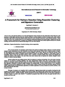
In multidimensional data, more than one variable is used and each has a different distribution. The relationship between Mahalanobis distance and chi-square distribution can be used to detect anomalies. The Mahalanobis distance from a data instance to the data mean is given by, MD(x) = (x − µ )T Σ−1 (x − µ ) where µ is the mean of the data and Σ is the d × d covariance matrix (d is the dimension of the data). For a d dimensional data generated from d Normal distributions, the square of the Mahalanobis distance follows a χd2 distribution, i.e. a chi-square distribution of d degree
CHAPTER 2. BACKGROUND
7
Figure 2.1: Chi-square distribution with 6 degrees of freedom. Those whose Mahalanobis distances are greater than 12.6 are considered anomalies of freedom. Figure 2.1 shows the chi-square distribution with 6 degrees of freedom. Notice the solid area in the long tail of the distribution: there is about 5% of the data whose Mahalanobis distances are greater than 12.6. In this case, it can be used as a cutoff to detect anomalies in the data. Consequently, to find anomalies in the multivariate data whose variables follow the Normal distributions, we can calculate the Mahalanobis distances q for all data instances. Those whose Mahalanobis distances are greater than inv( χd2 (1 − α )) are considered anomalies (α is the percentage of the small area in the long tail, e.g. α = 5%). Mahalanobis distance suffers from the effect where the data mean and covariance matrix are largely affected by significant anomalies. Using Mahalanobis distance to find anomalies in this case is unreliable. In order to avoid that effect, we need to determine the right statistical estimators for the data which are less sensitive to anomalies. The Minimum Covariance Determinant (MCD) proposed by Rousseeuw [57] is a wellknown approach to solve this problem. The MCD estimator is determined by finding from the data a subset of h data instances whose covariance matrix has the lowest determinant. The robust Mahalanobis distances are then computed based on the mean and covariance matrix of the h-size subset. The parameter h used in this way allows the estimator to resist the effect of the top n − h anomalous points.
CHAPTER 2. BACKGROUND
2.1.1.3
8
Weakness of Statistical Approach
The distribution-based approach assumes that the data distribution is known, which is often violated in practise. Extensive statistical tests to find an underlying distribution are also expensive. Moreover, statistical tests measuring anomalies based on how far they are from the mean will fail in the situation that anomalies locate near the mean position of the data.
2.1.2 Principal Component Based Approach Principal Component Analysis (PCA) is a vector space transformation from a high dimensional space to a lower dimensional space. PCA involves a calculation of the eigenvectors of a data covariance matrix, after removing the mean of the data for each feature. It is a simple and widely used method for dimensionality reduction. PCA maps original features from data onto a new set of axes which are called the principal components of the transformation. Each principal component is equivalent to an eigenvector of the covariance matrix of the original dataset. The first principal component corresponding to an eigenvector with a maximum eigenvalue is a linear combination of the original features with the largest variance. The second principal component is a linear combination of original features with the second largest variance and is orthogonal to the first principal component. The next ones have smaller variances and point to the directions of remaining orthogonal principal components. Typically first few principal components account for most of the variance in the data so that the rest of principal components can be skipped with a minimum loss of information. That is the main idea of using PCA to reduce dimensionality in data. The transformation works as follows. A dataset X is an n × d matrix where n is the number of data instances and d is the number of features. We can consider X a set of d column vectors X1 , X2 , ..., Xd . Each of them corresponds to values of a variable over n data instances. Likewise, each row of X, denoted as vectors x1 , x2 , ..., xn , corresponds to values of all features in a single data point. Suppose that X1 , X2 , ..., Xd have zero means, the covariance matrix of X is, C=
1 X T X. n−1
A matrix V whose columns are d eigenvectors of the covariance matrix C forms a
CHAPTER 2. BACKGROUND
9
set of d principal components. It is computed from the following decomposition, C = V DV T , where D is the diagonal matrix whose i-th diagonal element is the eigenvalue λi . By convention, eigenvectors in V have unit lengths and are sorted by their eigenvalues, from large to small (i.e. λ1 ≥ λ2 ≥ ... ≥ λd ). Suppose that r is the number of the first eigenvectors accounting for most of the variance of the data (r < d), let P (d × r) is a matrix formed by eigenvectors v1 , v2 , ..., vr as the columns. A projection of a data point xi onto a subspace spanned by eigenvectors in P, yi = PT xi , represents the PCA transformation of the the point xi . 2.1.2.1
Using PCA for Detecting Anomalies
A major problem in detecting anomalies in data which have more than one dimension (i.e. multivariate data) is that a data point may not be abnormal on any of the original features on their own, but can be an anomaly just because it is not compatible with the correlation structure of the remaining data. In that case, anomalies cannot be detected by considering only one original variable at a time. Anomalies can be captured by looking at directions defined by the first few or the last few principal components. Since the first few principal components capture most of the variance in the dataset, they are strongly related to one or more of the original features. As a result, data points which are anomalies on the direction of the first few principal components are usually anomalies on one or more of the original features as well. Anomalies in this case can be detected with distribution-based approach. In general, the last few principal components are more likely to contain information which does not conform to the normal data distribution [31]. They represent a linear combination of original features with very small variance. Thus the data tend to result in similar small values in those principal components. Therefore, any data instance that largely deviates from this tendency in the last few components is likely an anomaly. There are a number of statistical tests for anomalies using PCA. Rao proposed a test
CHAPTER 2. BACKGROUND
10
using the sum of squares of the values in the last q principal components [54], s2i =
d
∑
y2ik ,
k=d−q+1
where yik = vTk xi , where vk is the eigenvector corresponding to k-th principal component. As k increases, the variance of a principal component decreases and thus the value of yik tends to become smaller and contributes less to s2i . This may make the above test imprecisely in case some of the last principal components we have chosen have a very small variance compared with the others. Because those low-variance components mostly contribute to the detection of anomalies, their low contributions to s2i are not reasonable. To avoid this effect, we can give each principal component a weight equivalent to its variance [31], s2i
y2ik = ∑ , k=d−q+1 λk d
where λk is the eigenvalue of k-th principal components. When q = d, s2i =
y2ik ∑ λk = yTi D−1yi = yTi V T V D−1V T V yi, k=d−q+1 d
where V and D are defined in the previous section. V T = V −1 since V is an orthogonal matrix. Then, s2i = (yTi V T )(V D−1V T )(V yi ) = xiT C−1 xi . Therefore when q = d, s2i becomes the square of the Mahalanobis distance between point xi and the mean of the data sample. Recall that we have assumed that all data point xi have zero mean for simplicity. s2i is used to detect anomalies in the data. A data instance is considered anomaly if s2i is greater than a chosen threshold.
CHAPTER 2. BACKGROUND
2.1.2.2
11
Weakness of Principal Component Based Approach
The weakness of PCA is similar to the method using Mahalanobis distance in distributionbased approach. That is the anomalies themselves can affect the computation of principal components and we cannot get the correct principal components of the data. Moreover, PCA will also fail in the situation that anomalies locate near the center area of the data. That makes the anomalies look normal in the lower dimensional space of principal components. In addition, PCA has a high computational complexity O(d 3 ) when d is large (d is the number of features of the dataset).
2.1.3 Clustering-based Approach In clustering, data objects are clustered into groups so that objects in the same groups have high similarity, but very dissimilar to objects in other groups [26]. Anomalies can be detected using clustering techniques such as CLARANS [47], DBSCAN [19], and BIRCH [75] to make use of the fact that anomalies do not belong to any clusters. For example, DBSCAN proposed by Ester et al. is a density-based clustering techniques which grows regions with sufficient high density into clusters [19]. For each point of a cluster, the neighbourhood of a given radius has to contain at least a minimum number of points. This point is called a core object and its neighbour points are called directly density reachable from it. DBSCAN searches for a cluster by checking the neighbourhood of each point in the database, forming a cluster based on a core object, and collecting directly density reachable objects from the core object. Objects which do not belong to any cluster are considered anomalies. 2.1.3.1
Weakness of Clustering-based Approach
Anomaly detection is just a by-product of clustering techniques which are developed to optimize clustering and are often more computationally expensive compared with other anomaly detection methods.
2.1.4 Distance-based Approach Knorr and Ng proposed the definition of distance based DB(p, D) anomaly which does not make any assumption about the distribution of the data [34; 35]. The main idea is an object is an anomaly if it is far away from other data points in Euclidean distance.
CHAPTER 2. BACKGROUND
12
Specifically, an object o in a dataset T is a DB(p, D) anomaly if at least a fraction p of objects in T have greater distances than D from o. DB(p, D) anomalies can be determined by finding objects in D-neighbourhood of each object o. The authors also analysed how DB(p, D) anomalies generalize existing distribution-based techniques such as Normal distribution and Poisson distribution. For example, a point that lies outside three standard deviations from the mean is considered an anomaly assuming data follow a Normal distribution. This can be generalized by a DB(0.9988, 0.13σ ) where σ is the data standard deviation. A similar definition is DB(k, D) anomaly. An object o is a DB(k, D) anomaly if at most k objects have shorter distances than D from o. However, it is difficult to estimate suitable values of k and D and furthermore it is difficult to rank anomalies with these definitions. To address the problem, Ramawamay et. al. [53] proposed the definition of DB(k, N) anomaly which is based on the distance from an object to its k-th nearest neighbour. Anomalies are the top N data instances whose distances to their k-th nearest neighbours are largest. For all these methods, in order to estimate the abnormality for each data point, one needs to do the nearest neighbour search from that point. Therefore, it takes O(n2 ) time for all these methods. 2.1.4.1
Pruning Rule
In order to reduce the time to find the nearest neighbours, Bay and Schwabacher [5] proposed a simple but powerful pruning rule to find DB(k, N) anomalies: a data instance is not an anomaly if its distance to its k current nearest neighbours is less than the score of the weakest anomaly among top N anomalies found so far (examples of an anomaly score could be the minimum or average distance to its k nearest neighbours). This technique is useful if we only need to find top N anomalies where N is much smaller than the number of data instances. Suppose we have the anomaly scores of a set of N arbitrary points in the dataset. Let t be the smallest score in the set which is the average distance from the corresponding data point (i.e. the weakest anomaly) to its k nearest neighbours. Considering another point p which is not in the set. In order to compute an anomaly score of p, we need to find p’s k nearest neighbours by scanning through all the data points. However, during the scanning step, if we found p’s average distance to k neighbours is smaller than t, we can stop the scanning step since
CHAPTER 2. BACKGROUND
13
(a) Pruning example
(b) Anomaly has first ordering
(c) Anomaly has last ordering
(d) The best case
Figure 2.2: Different examples of pruning technique. p is already less abnormal than the current weakest one and thus does not belong to top N anomalies. Using this approach, a large number of non-anomalies can be pruned without carrying out a full data search. To have a better understanding of pruning rule and different situations of it, an example is made as in Figure 2.2. There is a dataset with 4 data points with distances as in Figure 2.2a. The number below each data point in Figures 2.2b, 2.2c, and 2.2d is its index in the dataset in three different cases. Assuming that an anomaly score for each point is a distance to its nearest neighbour and we want to find top N = 1 anomaly. It is clear that the leftmost point is an anomaly. We consider 3 situations in Figure 2.2b where the anomaly has the first ordering in the dataset, Figure 2.2c where the anomaly locates in the last index of the data, and Figure 2.2d where the ordering of the four points is the best case for this dataset using pruning. The analysis is described in Table 2.1. For a particular point, the nearest neighbour search scans through the data file from the beginning to the end until it stops by pruning or it reaches the end of the data. In the first situation, anomaly appears in the first index of the dataset. It takes 3 comparisons to know the anomaly score of point 1 is 2 which is the distance from point 1 to point 2. The weakest anomaly at this time is 1 and the weakest score is 2. Then it takes 2 comparisons to know the nearest neighbour of point 2 is point 1. Since it is smaller than the weakest anomaly score (2), the search stops. The analysis is similar for point 3. For point 4, it takes 3 comparisons to determine the score and no pruning happens. There are 10 comparisons in total to know point 1 is an anomaly in this case. In the second situation, since the anomaly appears at last, the weakest anomaly score
CHAPTER 2. BACKGROUND
14
Table 2.1: Different situations in using pruning rule. In the worst case when the anomaly locates in the end of the file, no point is pruned as a non-anomaly. In the best case, nonanomalies are pruned without carrying out an exhaustive nearest neighbour search. Index 1 2 3 4 1 2 3 4 1 2 3 4
Distance to knn Comparisons Weakest anomaly Weakest score Anomaly has first ordering (No. of comparisons = 10) 2 3 1 2 1 2 1 2 1 2 1 2 1 3 1 2 Anomaly has last ordering (No. of comparisons = 12) 1 3 1 1 1 3 1 1 1 3 1 1 2 3 4 2 The best case (No. of comparisons = 8) 1 3 1 1 2 3 2 2 1 1 2 2 1 1 2 2
is low at the beginning and still low in later steps and there is no pruning happening during the neighbour search for each point. This is the worst case for this dataset and it take 4 × 3 = 12 comparisons to know point 4 is an anomaly. The best case is the situation 3. The anomaly score is 3 for point 1 after 3 comparisons. It also takes 3 comparisons to know point 2 is more anomalous than point 1 and the weakest score is updated to 2. Since points 3 and 4 are near point 1, the beginning index, it takes only 1 comparison for both of them to know their scores are smaller than the weakest score. Therefore, the total number of comparisons is just 8. The details of the distance-based method using pruning rule to detect anomalies is described in Algorithm 1. 2.1.4.2
Weakness of Distance-based Approach
While the notion of distance-based anomaly set a stage for a distribution-free research in anomaly detection, this technique is capable of finding only global anomalies. For anomalies in data with different density regions, the density-based approach is more suitable.
CHAPTER 2. BACKGROUND
15
Algorithm 1: Distance-based Anomaly Detection with Pruning Technique Input: Data matrix X, the number of nearest neighbours k, the number of anomalies to return N Output: Top N anomalies 1: find the k nearest neighbours of each of the first N data points and their anomaly scores 2: t = the weakest anomaly score in the top N 3: for each of the remaining data points p in the dataset do 4: Keep track of the p’s nearest neighbours found so far 5: if p’s anomaly score < t then 6: p is not an anomaly, stop the nearest neighbour search, go to next point 7: end if 8: if p is compared with all the data points without any pruning then 9: Update the top N anomalies and t 10: end if 11: end for 12: Return top N anomalies
2.1.5 Density-based Approach The motivation of this method is illustrated in the dataset in Figure 2.3. This twodimensional dataset contains two clusters C1 and C2 . Cluster C1 is sparse, while cluster C2 is dense. It is not difficult to find that data point O1 , which stays far away from clusters C1 and C2 , is an anomaly. For point O2 , if we just compare it with the objects in cluster C2 , it is an DB(k, N) anomaly for a certain k and N. However, the problem becomes more complicated if we also consider cluster C1 . For the definition of DB(k, N) anomaly, if we define the parameters k and N so that O2 is an anomaly, then all data points in cluster C1 are anomalies. To solve this problem, Breunig et al. proposed the concept of density-based anomaly and a measure called LOF (Local Outlier Factor), which can pick up local anomalies [7]. Before defining LOF, some concepts need to be introduced. • k-distance of a data point p, denoted k-distance(p), is defined as a distance between p and its k-th nearest neighbour so that at least k data points are within the distance between p and k-th nearest neighbour and at most k − 1 data points are not in the boundary of the distance. • k-distance neighbourhood of an object p, denoted as Nk (p), consists of objects whose distances from p are not greater than the k-distance(p). Notice that the
CHAPTER 2. BACKGROUND
16
C1
O2 O1 C2
Figure 2.3: Global and local anomalies. O1 is a global anomaly since it is far away from all other data points. O2 is a local anomaly of cluster C2 . For the definition of DB(k, N) anomaly, if we define the parameters k and N so that O2 is an anomaly, then all data points in cluster C1 are anomalies. cardinality of Nk (p), denoted |Nk (p)|, is greater than k if p has more than one neighbour on the boundary of the neighbourhood. • The reachability distance of an object p with respect to an object o, denoted as reach-distk (p, o), is defined as max(k-distance(o), d(p, o)), where d(p, o) is the distance between p and o. Intuitively, if p and o are sufficient close, the reach-distk (p, o) is k-distance(o). If p is far from o, the reachability between two points is their distance. The reason for using the reachability distance is that the statistical fluctuation of d(p, o) for all the p’s close to o can be significantly reduced. It is controlled by the parameter k. • The local reachability density of an object p is defined as, µ
¶ ∑o∈Nk (p) reach-distk (p, o) lrdk (p) = 1/ . |Nk (p)| • Finally, the local outlier factor is defined as, lrd (o)
LOFk (p) =
∑o∈Nk (p) lrdkk(p) |Nk (p)|
.
The local outlier factor of a point p is an average ratio of the local reachability
CHAPTER 2. BACKGROUND
17
densities of p’s k-nearest neighbours and the local reachability density of p. It captures the degree to which p is an anomaly by looking at the densities of its neighbours. The lower p’s local reachability density and the higher local reachability densities of p’s k-nearest neighbours, the higher the LOF value of p. The authors have proved that the value of LOF is approximately equal to 1 for data points deep inside a cluster. Points with largest LOF values are marked as anomalies. Other variants of LOF have also been proposed. Papadimitriou et al. proposed LOCI, which used a measure called Multi-Granularity Deviation Factor (MDEF), a variation of LOF [49]. MDEF for a data instance is the relative deviation of its local neighbourhood density from the average local density in its neighbourhood of a given radius r. Sun, Chawla, and Arunasalam proposed other variants for detecting spatial anomalies in climate data and sequential anomalies in protein sequences [67; 13; 68]. 2.1.5.1
Weakness of Density-based Approach
Density-based approach can detect both global and local anomalies. However, the algorithm is computational expensive for large dataset. It takes O(n2 ) time to detect anomalies using LOF algorithm [11].
2.2
Random Walks on Graphs and Commute Time
2.2.1 Similarity Graph Many techniques utilizing graph model such as random walks and spectral clustering deal with a graph associated with the data. The issue that needs to be addressed is how to create such a similarity graph. Typically the graph should be able to model the neighbourhood relationship in the data. There are three typical similarity graphs: the ε -neighbourhood graph (connecting nodes whose distances are shorter than ε ), the fully connected graph (connecting all nodes with positive similarity with each other), and the k-nearest neighbour graph (connecting nodes u and v if u belongs to k-nearest neighbours of v or v belongs to k-nearest neighbours of u) [70]. A special case of the k-nearest neighbour graph is the ‘mutual’ knearest neighbour graph. This graph connects nodes u and v if u belongs to the k-nearest neighbours of v and v belongs to the k-nearest neighbours of u. The mutual k-nearest
CHAPTER 2. BACKGROUND
18
neighbour graph tends to connect nodes within a cluster of similar densities, but does not connect nodes from clusters of different densities [70]. Therefore, anomalies and clusters of different densities are isolated in the mutual k-nearest neighbour graph. The
ε -neighbourhood graph and (mutual) k-nearest neighbour graph with n nodes (k ¿ n) are usually sparse, which have advantages in computation. There are many ways to estimate the similarity between nodes in the graph such as Euclidean similarity, cosine similarity and Gaussian similarity. • Euclidean similarity: simeuclidean (i, j) = 1/dist(xi , x j ) where dist(xi , x j ) is an Euclidean distance between data points xi and x j . • Cosine similarity: simcosine (i, j) =
kxi kkx j k
where < xi , x j > is the dot product of
vectors xi and x j . −
• Gaussian similarity: simgaussian (i, j) = e
dist(xi ,x j )2 2σ 2
where σ is the kernel band-
width.
2.2.2 Random Walks on Graphs This section reviews basic concepts of random walks on graphs. Assume we are given a connected undirected and weighted graph G = (V, E,W ) with edge weights wi j ≥ 0 (i, j ∈ V ) and n nodes. Let A = (wi j )i, j∈V be the graph adjacency matrix. A degree of a node i is di = ∑ j∈N(i) wi j where N(i) is a set of neighbours of node i. We only concern nodes adjacent to i as for all other nodes j the weight wi j = 0. The volume of the graph is defined as vG = ∑i∈V di . Let D be a degree diagonal matrix with diagonal entries di∈V . A random walk is a sequence of nodes on a graph visited by a random walker: starting from a node, the random walker moves to one of its neighbour with some probability. Then from that node, it proceeds to one of its neighbour with some probability, and so on. The random walk is a finite Markov chain that is time-reversible, which means the reverse Markov chain has the same transition probability matrix as the original Markov chain [41]. The probability that the random walker from a node selects another node from its neighbours is decided by the weights of edges on the graph. The edge weight wi j is the similarity between nodes on graph mentioned in the Section 2.2.1. The larger the
CHAPTER 2. BACKGROUND
19
weight wi j of the edge connecting nodes i and j, the more often the random walker travels through this edge. The following is the probability that a random walker goes from state i at time t of the Markov chain to an adjacent state j at time t + 1: pi j = P(s(t + 1) = j|s(t) = i) =
wi j , di
Let P be the transition matrix with entry pi j . Then P = D−1 A. Denote πi (t) be the probability of reaching node i at time t, π (t) = [π1 (t), π2 (t), . . . , πn (t)]T be the state probability distribution at time t, the rule of walk is:
π (t + 1) = PT π (t), where T is the matrix transpose, and thus:
π (t) = (PT )t π (0), where π (0) is an initial state distribution.
π (0) is stationary if π (1) = π (0). In this case, π (t) = π (0), ∀t ≥ 0 and this walk is called the stationary walk [41]. For every graph G, the distribution π = [π1 , π2 , . . . , πn ]T where πi = di /vG is stationary:
π (1) = PT π (0) = (D−1 A)T π (0) = AT D−1 π (0) 1 = AT D−1 [d1 , d2 , . . . , dn ]T vG 1 1 = AT [1, . . . , 1]T = [d1 , d2 , . . . , dn ]T vG vG = π (0) As π (1) = π (0), the random walk is stationary and for every pair of nodes (i, j) the property of time-reversibility can be formulated as: πi pi j = π j p ji . That means the walker steps as often from i to j as from j to i [41].
CHAPTER 2. BACKGROUND
20
2.2.3 Hitting Time and Commute Time This section reviews two measures of random walks on graphs called hitting time hi j and commute time ci j [41]. The hitting time hi j is the expected number of steps a random walk starting at i will take to reach j for the first time: 0 hi j = 1 + ∑
k∈N(i) pik hk j
if i = j
(2.1)
otherwise.
The commute time is the expected number of steps that a random walk starting at i will take to reach j once and go back to i for the first time: ci j = hi j + h ji .
(2.2)
It is clear from Equations 2.1 and 2.2 that the commute time is symmetric while the hitting time is not. The commute time is a metric and thus is also called ‘commute time distance’. • ci j ≥ 0, • ci j = 0 if and only if i = j, • ci j = c ji , • ci j ≤ cik + ck j . There is a direct relationship between commute time and the effective resistance in electrical networks [18]. Consider an electrical network an undirected graph where each edge corresponds to a resistor with a conductance wi j . Then it is shown in [12] that ci j = vG ri j where ri j is the effective resistance between two nodes in the electrical network. Denote L = D − A be the graph Laplacian matrix. It has the following properties: • For every n dimensional vector v: vT Lv = 21 ∑i, j∈E wi j (vi − v j )2 • It is symmetric and positive semi-definite. • Its smallest eigenvalue is λ1 = 0 corresponding to an all-one eigenvector 1. • All the eigenvalues are real and non-negative (assume 0 = λ1 ≤ λ2 . . . ≤ λn ).
CHAPTER 2. BACKGROUND
21
For more details on graph Laplacian, refer to [16]. Denote L+ be the Moore-Penrose pseudo-inverse of L. Remarkably, the commute time can be computed from L+ [33; 20]. The reason of using the L+ is that L is not full rank: its first eigenvalue is zero. Therefore, L is not invertible. L+ can be written as [20],
1 1 L+ = (L − 11T )−1 + 11T . n n
(2.3)
Then the commute time is computed as, + ci j = vG (lii+ + l + j j − 2li j ),
(2.4)
where li+j is the (i, j) element of L+ . Equation 2.4 can be written as ci j = vG (ei − e j )T L+ (ei − e j ),
(2.5) 1/2
where ei is the i-th column of an (n × n) identity matrix I [59]. Consequently, ci j is a distance in the Euclidean space spanned by the ei ’s. We do not really need to do the pseudo inversion of L+ in order to calculate ci j . Because the Laplacian matrix L (n × n) is symmetric and has rank n − 1 [16], it can be decomposed as L = V SV T , where V is the matrix containing eigenvectors of L as columns and S is the diagonal matrix with the corresponding eigenvalues on the diagonal. Then L+ = V S−1V T . Therefore, li+j =
n
1
∑ λk vik v jk ,
(2.6)
k=2
where vi j is the (i, j) entry of V . The followings are examples of some special unweighted graphs and their commute time. Example 1 For a complete graph of n nodes, which has edge set {(u, v) : u 6= v}, ci j = 2(n − 1), ∀1 ≤ i, j ≤ n and i 6= j. Example 2 For a star graph of n nodes, which has edge set {(k, v) : 1 ≤ k ≤ n and v 6=
CHAPTER 2. BACKGROUND
k},
2(n − 1) if i = k and j 6= k ci j = 4(n − 1) if i 6= k and j = 6 k and i 6= j.
Example 3 For a path of n nodes, which has edge set {(u, u + 1) : 1 ≤ u < n)}, ci j = 2( j − i)(n − 1), ∀1 ≤ i < j ≤ n.
22
Chapter 3 Robust Anomaly Detection Using Commute Time This chapter is based on the following publication: Robust Outlier Detection Using Commute Time and Eigenspace Embedding Nguyen Lu Dang Khoa and Sanjay Chawla In proceedings of the 14th Pacific-Asia Conference on Knowledge Discovery and Data Mining (PAKDD ’10), Hyderabab, India, 2010, pp. 422-434.
3.1
Introduction
In Chapter 2, we summarize the anomaly detection techniques, their strengths and weaknesses. Standard techniques for anomaly detection include statistical [27; 58; 4], distance-based [34; 35; 5] and density-based [7] approaches. However, standard statistical and distance-based approaches can only find global anomalies. A well-known method for detecting local anomalies is the Local Outlier Factor (LOF), which is a density-based approach [7]. The downside of LOF is its expensive computational time O(n2 ) [11]. Recently, Moonesinghe and Tan [45] proposed a method called OutRank to detect anomalies using random walks on graphs. The anomaly score is the connectivity of each node which is computed from a stationary random walk. This method
23
CHAPTER 3. ROBUST ANOMALY DETECTION USING COMMUTE TIME
24
Figure 3.1: Example of commute time. Edge e12 has a larger commute time than all edges in the cluster while its Euclidean distance is the same or smaller than their Euclidean distances. Table 3.1: The Euclidean distance and the commute time for the graph in Figure 3.1. The commute times between inter-cluster nodes are significantly larger than the commute times between intra-cluster nodes compared to the Euclidean distances. Index 1 2 3 4 5
Euclidean Distance 1 2 3 4 0 1.00 1.85 1.85 1.00 0 1.00 1.00 1.85 1.00 0 1.41 1.85 1.00 1.41 0 2.41 1.41 1.00 1.00
5 2.41 1.41 1.00 1.00 0
1 0 12.83 19.79 19.79 20.34
Commute Time Distance 2 3 4 12.83 19.79 19.79 0 6.96 6.96 6.96 0 7.51 6.96 7.51 0 7.51 6.96 6.96
5 20.34 7.51 6.96 6.96 0
cannot find anomalous clusters where the node connectivities are still high. An excellent survey by Chandola et. al [11] provides a more detailed view on anomaly detection techniques. In this chapter, we present a new method to find anomalies using a measure called ‘commute time’ or ‘commute time distance’ which is described in Chapter 2. Our interest is inspired by the use of commute time as a metric for anomaly detection. Indeed the commute time is an Euclidean distance in the space spanned by eigenvectors of the graph Laplacian matrix. Unlike traditional Euclidean distance, commute time between two nodes can capture both the distance between them and the data densities so that we can capture both global and local anomalies using distance-based methods such as methods in [5; 34]. Moreover, the method can be applied directly to graph data. To illustrate, consider a graph of five data points shown in Figure 3.1. Denote dED (i, j) and dCD (i, j) be an Euclidean distance and a commute time between points i and j, respectively. The distances between all pairs of data points are in Table 3.1. It can be seen that dCD (1, 2) is much larger than dCD (i, j) ((i, j) ∈ {2, 3, 4, 5}, i 6=
CHAPTER 3. ROBUST ANOMALY DETECTION USING COMMUTE TIME
25
14000 Inter−cluster distance Average intra−cluster distance
Commute time distance
12000
10000
8000
6000
4000
2000
0
0
20
40
60 80 Number of new points
100
120
Figure 3.2: Example showing commute time can capture the data density where an anomaly connects to a ball cluster of 200 data points. The more points added to the cluster, i.e. the denser the cluster, the commute time between the anomaly and the cluster (inter-cluster commute time) changed dramatically while the average pair-wise commute times between all pairs of nodes in the cluster (intra-cluster commute time) just slightly changed. j) even though dED (i, j) have the same or larger Euclidean distances than dED (1, 2). The commute times from a node outside the cluster to nodes inside the cluster are significantly larger than the pairwise commute times of nodes inside the cluster. Since commute time is a metric, a distance-based method can be used to realize that node 1 is far away from other nodes using commute time. Another example is the case of an anomaly connecting to a ball cluster of 200 data points. We gradually added a sequence of 100 new points to the ball cluster. The result in Figure 3.2 turned out that the more points added to the cluster, i.e. the denser the cluster, the commute time between the anomaly and the cluster changed dramatically while the average of pair-wise commute times between all pairs of nodes in the cluster just slightly changed. This shows commute time between two points captures not only the distance between them but also their data densities. Therefore, the use of commute time is promising for identifying anomalies. The contributions of this work are as follows: • We prove that commute time can naturally capture the data density and establish
CHAPTER 3. ROBUST ANOMALY DETECTION USING COMMUTE TIME
26
a relationship between commute time and local anomaly detection. • We propose a distance-based anomaly detection method using the commute time metric to detect global and local anomalies. The method can also detect group anomalies which traditional methods often fail to capture. • We accelerate the computation of commute time using graph component sampling and eigenspace approximation to avoid the O(n3 ) eigen decomposition of the graph Laplacian. Furthermore, making use of the distance-based method, pruning technique is used to reduce the computation. All of them speed up the method significantly to O(nlogn) while preserving the anomaly ranking. • We show the effectiveness of the methods in synthetic and real datasets in many application domains. The results show that commute time is a promising measure for anomaly detection. The remainder of the chapter is organized as follows. In Section 3.2, we introduce a method to detect anomalies using the commute time measure. Section 3.3 presents a method to approximate the commute time and accelerate the algorithm. In Section 3.4, we evaluate our approach and analyze the results using experiments on synthetic and real datasets. Section 3.5 is the summary of the chapter.
3.2
Commute Time Distance Based Anomaly Detection
3.2.1 A Proof of Commute Time Property for Anomaly Detection We now show that the commute time can capture the data density and is a good metric for local anomaly detection. Lemma 1 The expected number of steps that a random walk which has just visited node i will take before returning back to i is vG /di . Proof 1 It is known that a distribution π = [π1 , π2 , ..., πn ]T where πi = di /vG is stationary [41]. As the random walk is stationary, if it has just visited node i, the expected number of steps it will take before returning back to i is: 1/πi = vG /di .
CHAPTER 3. ROBUST ANOMALY DETECTION USING COMMUTE TIME
s
27
t
(a)
(b)
Figure 3.3: The commute time from an anomaly to a node in a cluster increases when the cluster is denser. Theorem 1 Given a cluster C and a point s outside C connected to a point t of C (Figure 3.3a). If C becomes denser (by adding more points or edges), the commute time between s and t increases. Proof 2 From Lemma 1, the expected number of steps that a random walk which has just visited node s will take before returning back to s is vG /ds = vG /wst . Since the random walk can only move from s to t and come back to s from t, vG /wst = hst + hts = cst (Figure 3.3b). If cluster C becomes denser, there are more edges in cluster C. As a result, vG increases while wst is unchanged. So the commute time between s and t (i.e. cst ) increases. As shown in Theorem 1, the denser the cluster, the larger the commute time between a point s outside the cluster to a point t in the cluster. Therefore, the commute time can capture the data density and we can use this property to effectively detect local anomalies using the commute time.
3.2.2 Anomaly Detection Using Commute Time This section introduces a method based on commute time to detect anomalies. As commute time is a metric and captures both the distance between nodes and the data density, we can use a commute time distance based method to find global and local anomalies. The detail of the method is described in Algorithm 2. First, a mutual k1 -nearest neighbour graph G is constructed from the dataset. If the data have coordinates, we can use kd-tree to avoid O(n2 ) searching of nearest neighbours. However, it is possible that the mutual k1 -nearest neighbour graph is not connected so that we cannot apply random walk on the whole graph. One approach to make the graph connected is to find its
CHAPTER 3. ROBUST ANOMALY DETECTION USING COMMUTE TIME
28
minimum spanning tree and add the edges of the tree to the graph. Given a connected and undirected graph, a spanning tree of that graph is a subgraph connecting all the vertices together. A minimum spanning tree is a spanning tree with minimum weight. Therefore, an addition of G and a minimum spanning tree of a fully connected graph corresponding to G will form a connected graph. Algorithm 2: Commute Time Distance Based Anomaly Detection Input: Data matrix X, the numbers of nearest neighbours k1 (for building the knearest neighbour graph) and k2 (for estimating the anomaly score), the numbers of anomalies to return N Output: Top N anomalies 1: Construct the mutual k-nearest neighbour graph G from the dataset (using k1 ) 2: Compute the graph Laplacian matrix L and its pseudoinverse L+ 3: Find top N anomalies using the distance-based technique on commute time with pruning rule (using k2 ) described in Algorithm 1. The commute time between two nodes i and j can be computed using Equation 2.4 4: Return top N anomalies Then the graph Laplacian matrix L and its pseudoinverse L+ are computed. After that the pairwise commute times between any two nodes can be calculated from L+ . Finally, a distance-based anomaly detection using commute time with pruning technique described in Algorithm 1 is used to find the top N anomalies. Recall that the main idea of pruning is that a data point is not an anomaly if its average distance to k2 current nearest neighbours is less than the score of the weakest anomaly among top N anomalies found so far. Using this approach, a large number of non-anomalies can be pruned without carrying out a full data search. The anomaly score used is the average distance of a node to its k2 nearest neighbours. Suitable values for k1 (for building the nearest neighbour graph) and k2 (for estimating the anomaly score) will be presented in the experiments.
3.3
Graph Component Sampling and Eigenspace Approximation
While commute time is a robust measure for detecting both global and local anomalies, the main drawback is its computational time. The direct computation of commute time involves the eigen decomposition of the graph Laplacian matrix which is proportional
CHAPTER 3. ROBUST ANOMALY DETECTION USING COMMUTE TIME
29
to O(n3 ) and is not feasible to use in large graphs (n is the number of nodes). In this work, the graph components are sampled to reduce the graph size and then eigenspace approximation in [59] is applied to approximate the commute time on the sampled graph.
3.3.1 Graph Sampling An easy way to sample a graph is selecting nodes from it uniformly at random. However, sampling in this way can break the graph geometry structure and anomalies may not be chosen after sampling. To resolve this, we propose a sampling strategy called component sampling. After creating the mutual k1 -nearest neighbour graph, the graph tends to have many connected components corresponding to different data clusters. Anomalies are likely isolated nodes or nodes in very small components. For nodes in normal components (we have a threshold to distinguish between normal and anomalous components), they are uniformly sampled with the same ratio p = 50k1 /n, which is chosen from preliminary experimental results. For nodes in anomalous components, we leave all of them intact. Then we rebuild a mutual k1 -nearest neighbour graph for the sampled data. Sampling in this way will maintain the geometry of the original graph and the relative densities of normal clusters. Anomalies are also not discarded in this sampling strategy.
3.3.2 Eigenspace Approximation Equation 2.5 can be written as: ci j = vG (ei − e j )T L+ (ei − e j ) = vG (ei − e j )T V S−1V T (ei − e j ) = vG (ei − e j )T V S−1/2 S−1/2V T (ei − e j ) √ √ = [ vG S−1/2V T (ei − e j )]T [ vG S−1/2V T (ei − e j )]. Let xi = S−1/2V T ei , ci j = vG (xi − x j )T (xi − x j ).
(3.1)
Therefore, the commute time between nodes on the graph can be viewed as the squared Euclidean distance in the node space spanned by eigenvectors of the graph
CHAPTER 3. ROBUST ANOMALY DETECTION USING COMMUTE TIME
30
Laplacian matrix. Denote V˜ , S˜ be a matrix containing m largest eigenvectors of L+ and its corresponding diagonal matrix, and x˜i = S˜−1/2V˜ T ei , the approximate commute time is c˜i j = vG (x˜i − x˜ j )T (x˜i − x˜ j ).
(3.2)
The commute time ci j in an n dimensional space is transformed to the commute time c˜i j in an m dimensional space. Therefore, we just need to compute the m smallest eigenvectors with nonzero eigenvalues of L (i.e. the largest eigenvectors of L+ ) to approx+ imate the commute time. This approximation is bounded by kci j − c˜i j k ≤ vG ∑m i=1 λi
[59].
3.3.3 Algorithm The proposed method is outlined in Algorithm 3. We create the sampled graph from the data using graph components sampling. Then the graph Laplacian Ls of the sampled graph and matrix V˜ (m smallest eigenvectors with nonzero eigenvalues of Ls ) are computed. Since we use the pruning technique, we do not need to compute the approximate commute time for all pairs of points. Instead, we compute it ‘on demand’ using Equation 2.4 where l˜i j = ∑m 1 vik v jk , and vi j is (i, j) entry of matrix V˜ . k=2 λk
Algorithm 3: Commute Time Distance Based Anomaly Detection with Graph Component Sampling and Eigenspace Approximation Input: Data matrix X, the numbers of nearest neighbours k1 and k2 , the numbers of anomalies to return N Output: Top N anomalies 1: Construct the mutual k1 -nearest neighbour graph from the dataset 2: Do the graph component sampling 3: Reconstruct the mutual k1 -nearest neighbour graph from sampled data 4: Compute the Laplacian matrix of the sampled graph and its m smallest eigenvectors 5: Find top N anomalies using the commute time based technique with pruning rule (using k2 ) 6: Return top N anomalies
CHAPTER 3. ROBUST ANOMALY DETECTION USING COMMUTE TIME
31
3.3.4 The Complexity of the Algorithm The k-nearest neighbour graph with n nodes is built in O(n log n) using kd-tree with the assumption that the dimensionality of the data is not very high. The average degree of each node is O(k) (k ¿ n). So the graph is sparse and thus finding connected components take O(kn). After sampling, the size of graph is O(ns ) (ns ¿ n). The standard method for eigen decomposition of Ls is O(n3s ). Since Ls is sparse, it would take O(Nns ) = O(kn2s ) where N is the number of nonzeros. The computation of just the m smallest eigenvectors (m < ns ) is less expensive than that. The typical distance-based anomaly detection takes O(n2s ) for the neighbourhood search. Pruning can scale it nearly linear [5]. We only need to compute the commute times O(ns ) times each of which takes O(m). So the time needed for two steps is proportional to O(n log n + kn + kn2s + mns ) = O(n log n) as ns ¿ n.
3.4
Experiments and Analysis
In this section, the effectiveness of commute time as a measure for anomaly detection was evaluated in synthetic and real datasets. We also analyzed some properties of the proposed method and the impact of its parameters.
3.4.1 Synthetic Datasets 3.4.1.1
An illustrated example
In the following experiment, the ability of the distance-based technique using commute time (denoted as CDOF) in finding global, local anomalies, and group anomalies was evaluated in a synthetic dataset. The distance-based technique using Euclidean distance [5] (denoted as EDOF), LOF [7], and OutRank [45] (denoted as ROF and the same graph of CDOF was used) were also used to compare with CDOF. Figure 3.4 shows a 2-dimensional synthetic dataset. It contains one dense cluster of 500 data points (C1 ) and one sparse cluster of 100 data points (C2 ). Moreover, there are three small anomalous clusters with 12 data points each (C3−5 ) and four anomalies (O1−4 ). All the clusters were generated from Normal distribution. O2 , O3 , and O4 are
CHAPTER 3. ROBUST ANOMALY DETECTION USING COMMUTE TIME
C5
90
32
C2
80 O1 O2
70
60
C1 C3
O3
50
40
C4
O4
30
40
50
60
70
80
90
100
Figure 3.4: The synthetic dataset with normal clusters (C1−2 ), anomalies (O1−4 ), and anomalous clusters (or group anomalies C3−5 ). O2 , O3 , and O4 are global anomalies which are far away from other clusters. O1 is a local anomaly of dense cluster C1 . global anomalies which are far away from other clusters. O1 is a local anomaly of dense cluster C1 . In the experiment for this dataset, the numbers of nearest neighbours were k1 = 10 (for building the graph), k2 = 15 (for estimating the anomaly score. Since the size of outlying clusters is twelve, fifteen was a reasonable number to estimate the anomaly scores), and the number of top anomalies was N = 40 (the total data points in three outlying clusters and four anomalies). The results are shown in Figure 3.5. The ‘x’ signs mark the top anomalies found by each method. The figure shows that EDOF cannot detect local anomaly O1 . Both EDOF and LOF cannot find two outlying cluster C3 and C4 . The reason is those two clusters are near each other with similar densities and consequently for each point in the two clusters the average distance to its nearest neighbours is small and the relative density is similar to that of its neighbours. Moreover, ROF anomaly score is actually the node probability distribution when the random walk is stationary [45]. Hence it is di /vG [41], which is small for anomalies 1 . Therefore, it cannot capture nodes in the outlying clusters where di is large. For degree-one outlying nodes, ROF and CDOF have similar scores. The result in Figure 3.5d shows that CDOF 1 This
score has not been explicitly stated in the ROF paper.
CHAPTER 3. ROBUST ANOMALY DETECTION USING COMMUTE TIME
90
90
80
80
70
70
60
60
50
50
40
40
30
40
50
60
70
80
90
100
30
40
50
(a) EDOF
90
80
80
70
70
60
60
50
50
40
40
40
50
60
70
70
80
90
100
80
90
100
(b) LOF
90
30
60
33
80
90
100
(c) ROF
30
40
50
60
70
(d) CDOF
Figure 3.5: Comparison of the results of EDOF, LOF, ROF, and CDOF. CDOF can detect all global, local anomalies, and even group anomalies effectively. can identify all the anomalies and anomalous clusters. The key point is in commute time, inter-cluster distance is significantly larger then intra-cluster distance even if the two clusters are near in the Euclidean distance. 3.4.1.2
Effectiveness of the Proposed Method
In this section, we show the effectiveness of the proposed method in terms of performance and accuracy. In the following experiment, we compared the performances of EDOF, LOF, and approximate CDOF mentioned in Section 3.3. The experiment was performed using five synthetic datasets, each of which contained different clusters generated from Normal distributions and a number of random points generated from uniform distribution, which were likely anomalies. The sizes and the locations of the
CHAPTER 3. ROBUST ANOMALY DETECTION USING COMMUTE TIME
34
4
3
x 10
EDOF LOF CDOF
2.5
Time (s)
2
1.5
1
0.5
0
1
1.5
2
2.5
3 Data sizes
3.5
4
4.5
5 4
x 10
Figure 3.6: Performances of EDOF, LOF, and approximate CDOF. This reflects the complexities of O(n), O(n log n), and O(n2 ) for EDOF, approximate CDOF, and LOF, respectively. generated clusters were also chosen randomly. The data generation for each dataset stopped when the current number of data points equaled to a predefined data size. The results are shown in Figure 3.6 where the horizontal axis represents the dataset sizes in the ascending order and the vertical axis is the corresponding computational time. The result of approximate CDOF was averaged over ten trials of data sampling. It is shown that approximate CDOF is faster than LOF and slower than EDOF. This reflects the complexities of O(n), O(n log n), and O(n2 ) for EDOF, approximate CDOF, and LOF, respectively. In order to validate the accuracy of the approximate commute time method, we used commute time and approximate commute time to find anomalies in five synthetic datasets generated in the same way as the experiment above with smaller sizes due to the expensive computation of CDOF. The results were averaged over ten trials and shown in Figure 3.7. The red and green curves shows the computational time of CDOF and approximate CDOF (aCDOF) which corresponds to the right vertical axis while the blue bar shows the percentage of top anomalies found by aCDOF among top anomalies found by CDOF which corresponds to the left vertical axis. The figure shows that aCDOF is much faster than CDOF but still preserves a high percentage (84.6% on
CHAPTER 3. ROBUST ANOMALY DETECTION USING COMMUTE TIME
100
35
800
90
700
80 600
500
60
50
400
40
CD
OF
Time (s)
Outlier Percentage (%)
70
300
30 200 20
10
0
aC 1000
2000
100
F DO
3000 Data Sizes
4000
5000
0
Figure 3.7: Effectiveness of the approximate CDOF. Approximate CDOF is much faster than exact CDOF but still preserves the detection accuracy. average) of top anomalies found by CDOF.
3.4.2 Real Datasets 3.4.2.1
Basketball Dataset
In this experiment, CDOF was used to find anomalies in an NBA dataset which is available at http://www.databasebasketball.com. The dataset contains information of all the players in the well-known basketball league in the US in year 1997-1998. There were 547 players and six features were used: position, points per game, rebounds per game, assists per game, steals per game and blocks per game. Point and assist reflect the offensive ability of a player while steal and block show how good a player is in defending. Rebound can be either offensive or defensive but total rebound is usually an indicator of defensive ability. We chose the number of nearest neighbours k1 = 10 to build the mutual nearest neighbour graph, k2 = 10 to estimate the anomaly score. The results are shown in Table 3.2 with the ranking and statistics of top five anomalies. The table also shows the maximums, averages, and standard deviations for each attribute over all players. Dikembe Mutombo was ranked as the top anomaly. He had the second highest
CHAPTER 3. ROBUST ANOMALY DETECTION USING COMMUTE TIME
36
Table 3.2: The anomalous NBA players. Rank 1 2 3 4 5
Player Dikembe Mutombo Dennis Rodman Michael Jordan Shaquille O’neal Jayson Williams Max Average Standard deviation
Position Center Forward Guard Center Forward
Points 13.43 4.69 28.74 28.32 12.88 28.74 7.69 5.65
Rebounds 11.37 15.01 5.79 11.35 13.58 15.01 3.39 2.55
Assists 1.00 2.88 3.45 2.37 1.03 10.54 1.78 1.77
Steals 0.41 0.59 1.72 0.65 0.69 2.59 0.70 0.48
Blocks 3.38 0.23 0.55 2.40 0.75 3.65 0.40 0.53
blocks (5.6 times of standard deviation away from mean), the highest rebounds for center players, and high points. It is rare to have good scores in three or more different statistics and he was one of the most productive players. Dennis Rodman and Michael Jordan took the second and third positions because of their highest scores in rebound and point (4.6 and 3.7 times of standard deviation away from mean, respectively). Dennis Rodman was a rare case because his points were quite low among high rebound players as well. The next was Shaquille O’Neal who had the second highest points and high rebounds. He was actually the best scoring center and is likely a local anomaly among center players. Finally, Jayson Williams had the second highest rebounds. It is interesting to note that except for Dennis Rodman because of his bad behaviour in the league, the other four players were listed in that year as members of All-Stars team. 3.4.2.2
Spam Dataset
The spambase dataset provided by Machine Learning Repository [22] was used. There are 4,601 emails in the data with 57 features each. Most of the features (54) indicate the frequency of occurring of a particular word or character in the email. Only three other features measure the length of sequences of consecutive capital letters. The task is checking whether an email is a spam or not. EDOF, LOF, and CDOF were applied on this dataset. We chose the number of nearest neighbours k1 = 10 to build the mutual nearest neighbour graph for CDOF, k2 = 20 to estimate the anomaly score for all three methods. There were top N = 100 anomalies to be detected. The result shows the detection accuracy were 84% for EDOF, 23% for LOF, and 92% for CDOF. So CDOF outperformed other methods in detecting email spam. The result shows that in this dataset, most of local anomalies detected were not spam. Since
CHAPTER 3. ROBUST ANOMALY DETECTION USING COMMUTE TIME
37
25 EDOF LOF CDOF
Feature score
20
15
10
0
make address all 3d our over remove internet order mail receive will people report addresses free business email you credit your font 000 money hp hpl george 650 lab labs telnet 857 data 415 85 technology 1999 parts pm direct cs meeting original project re edu table conference ; ( [ ! $ # cap−avg cap−max cap−sum
5
Feature name
Figure 3.8: Feature analysis of spam dataset. A feature score is a ratio of the average of the feature values in top N = 100 anomalies detected by the method and the average of the feature values in all data instances. most of the features are frequencies of words or characters which are also indicators of spam or non-spam, we made an feature analysis for all methods and the results were shown in Figure 3.8. A feature score is a ratio of the average of the feature values in top N = 100 anomalies detected by the method and the average of the feature values in all data instances. The reason to normalize by the average of the feature values in all data instances was some features had high frequencies in all data instances and thus always had high scores in all methods. Table 3.3 shows in descending order top fifteen features by their scores for each method. Both the results show that features with dominant values in EDOF and CDOF are likely the indicators of spam while features with dominant values in LOF are likely the indicators of non-spam.
3.4.3 Real Graph Data As already noted, one advantage of CDOF over other methods is it can work directly with graph data while many others cannot. In this section, CDOF were applied directly to a graph dataset - the DBLP co-authorship network. In this graph, nodes are authors and edge weights are the number of collaborated papers between the authors. Since the graph is not fully connected, we extracted its biggest component. It has 612,949
CHAPTER 3. ROBUST ANOMALY DETECTION USING COMMUTE TIME
38
Table 3.3: Top 15 features for each method in spam dataset. It shows that features with dominant values in EDOF and CDOF are likely the indicators of spam while features with dominant values in LOF are likely the indicators of non-spam. Index 1 2 3 4 5 6 7 8 9 10 11 12 13 14 15
EDOF Feature Score cap-avg 16.32 cap-max 12.19 cap-sum 8.91 report 5.25 order 3.52 addresses 3.46 000 3.39 $ 3.32 credit 3.10 make 3.08 money 2.92 mail 2.56 people 2.45 receive 2.15 3d 2.14
LOF Feature Score address 23.37 project 8.17 cap-avg 7.72 parts 6.31 cap-max 4.97 [ 3.37 free 3.25 conference 3.16 cap-sum 3.07 credit 2.90 meeting 2.77 george 2.53 telnet 1.93 85 1.91 our 1.90
CDOF Feature Score 3d 20.18 cap-avg 15.45 cap-max 13.07 cap-sum 7.98 credit 6.92 report 5.80 addresses 4.91 order 3.67 000 3.48 font 3.43 $ 3.37 money 2.74 receive 2.71 make 2.24 mail 2.20
nodes and 2,345,178 edges in a snapshot in December 5th, 2011 which is available at http://dblp.uni-trier.de/xml/. Since this graph is too big to do a qualitative analysis, a subset of the graph in main data mining conferences was extracted. We selected only authors and publications appearing in KDD, PKDD, PAKDD, ICDM, and SDM. Each author also needs to have at least 10 publications and his/her co-authors need to have such minimum publications as well. This selected only authors who published highly in major data mining conferences and collaborated with the similar kind of co-authors. Then the biggest connected component of the graph was extracted. The final graph has 397 nodes and 1,695 edges. The average node degree is 4.27 and the average node weight is 10.48. On further inspection of the top anomalies found by CDOF, authors 321, 342, 318, 129, 340, 336, 354, 7, 349, 322, 83, and 355 were the top 12 anomalies shown in Figure 3.9 where a dash line separated an anomalous part and the remaining of the graph. Among those, besides authors 321, 322, and 240, there were two group anomalies detected. They are cliques of four and six nodes and corresponding to two research groups
CHAPTER 3. ROBUST ANOMALY DETECTION USING COMMUTE TIME
39
7
129
342
349
83
355
372
336
318
354 321
340 322
Figure 3.9: Anomalies in DBLP data mining co-authorship network. There were two group anomalies detected which are cliques of four and six nodes corresponding to two research groups in Nanyang Technological University Singapore (NTU) and North Dakota State University (NDSU), respectively. in Nanyang Technological University Singapore (NTU) and North Dakota State University (NDSU), respectively. The reasons they were detected as group anomalies is that each of them had a strong collaboration inside the group but did not have a strong collaboration to researchers outside the group. This is not a popular situation for highly published researchers. Normally a group leader, e.g. a professors, have collaborations with not only group members (e.g. research students or postdoctoral fellows) but also other researchers in the research community.
3.4.4 Relationship between LOF, EDOF, and CDOF In this section, we investigate the ranking of LOF, EDOF, and CDOF and the relationship between them using five synthetic datasets generated in the same way as the previous sections. We computed anomaly scores of all data instances using the three methods. Then Spearman rank test [63] was applied to check the correlation between the rankings of anomalies in the three methods. The result is shown in Figure 3.10. To aid the analysis, the anomaly scores of the three methods in the dataset in section 3.4.1 were plotted in Figure 3.11. CDOF and EDOF have very high correlation in ranking because both of them basically use distance as a measure. Data points in the same clusters have similar scores
CHAPTER 3. ROBUST ANOMALY DETECTION USING COMMUTE TIME
40
1
0.9
EDOF vs. LOF EDOF vs. CDOF LOF vs. CDOF
Spearman rank
0.8
0.7
0.6
0.5
0.4
1000
1500
2000
2500 3000 3500 Dataset sizes
4000
4500
5000
Figure 3.10: Relationship among EDOF, LOF, and CDOF. CDOF and EDOF have high correlation in ranking because both of them use distance as a measure of anomaly scores. LOF correlates more with CDOF than EDOF because both of them take densities into account and can detect local anomalies. except anomalies and points in border regions of clusters. Specifically, data points in sparse clusters have high scores and data points in dense clusters have low scores. The difference between the two methods is CDOF scores of local anomalies in dense regions can be higher than normal points in sparse regions. The reason LOF does not have high rank correlation with CDOF and EDOF is LOF uses density to score anomalies. Most of data points inside cluster have LOF of about 1 except anomalies and data points in the border of the cluster. Moreover, LOF correlates more with CDOF than EDOF because both of them take data densities into account and can detect local anomalies. The experiment in this section shows that the commute time simultaneously captures both distance and density in data and thus is able to detect both global and local anomalies. The anomaly scores in Figure 3.11 also show that by using commute time we can recognize the structure of the data easily. We can easily see the dense and sparse clusters, two nearby outlying clusters, an isolated outlying cluster, and the four anomalies by CDOF score. That illustrates why CDOF outperforms others in anomaly detection.
CHAPTER 3. ROBUST ANOMALY DETECTION USING COMMUTE TIME
41
16 14 12
EDOF
10 8 6 4 2 0
0
100
200
300 400 Data point ids
500
600
700
500
600
700
500
600
700
(a) EDOF 5 4.5 4 3.5
LOF
3 2.5 2 1.5 1 0.5
0
100
200
300 400 Data point ids
(b) LOF 4
8
x 10
7 6
CDOF
5 4 3 2 1 0
0
100
200
300 400 Data point ids
(c) CDOF
Figure 3.11: Anomaly factors of EDOF, LOF, and CDOF. Data points in the same clusters have similar EDOF and CDOF scores. The difference is CDOF scores of local anomalies in dense regions can be higher than normal points in sparse regions. For LOF, most of data points inside cluster have LOF of about 1.
CHAPTER 3. ROBUST ANOMALY DETECTION USING COMMUTE TIME
42
4
x 10 15
10
10
5
5
CDOF
Degree
15
0
0
100
200
300 400 Data point ids
500
600
0 700
Figure 3.12: Commute time and node degree. High degree nodes can have high anomaly scores and low degree nodes can have low anomaly scores. We cannot simply detect anomalies by using their node degrees.
3.4.5 Commute Time and Node Degree It is likely that anomalies are isolated nodes in the nearest neighbour graph and have low node degrees. One might say that we can only need the node degree information to decide if a node is an anomaly or not. To validate this claim, we plotted the anomaly score of every node corresponding to its degree sorted in descending order of the dataset in Section 3.4.1. The result is in Figure 3.12. It shows that high degree nodes can have high anomaly scores and low degree nodes can have low anomaly scores. Some examples for those cases are anomalies in outlying clusters can have high degrees or normal nodes in the boundary of normal clusters can have low degrees. Using the anomaly scores based on commute time, we can detect anomalies properly in those situations.
3.4.6 Impact of Parameters In this section, we investigate how the number of nearest neighbours affects CDOF. Denote kmin be the maximum number of nodes that a cluster is an outlying cluster and kmax be the minimum number of nodes that a cluster is a normal cluster. There are
CHAPTER 3. ROBUST ANOMALY DETECTION USING COMMUTE TIME
43
100 EDOF LOF CDOF
90
80
Precision
70
60
50
40
30
20
10
0
10
20
30
40
50 k2
60
70
80
90
100
Figure 3.13: The detection results with different k2 in estimating anomaly scores for the dataset in Section 3.4.1. The same result for CDOF can also be obtained with 15 < k2 < 100. CDOF is more robust than EDOF and LOF in terms of changes in parameters. two situations. If we choose the number of nearest neighbours k2 < kmin , nodes in an outlying cluster do not have neighbours outside the cluster. As a result, their anomaly scores are small and we will miss them as anomalies. On the other hand, if we choose k2 > kmax , nodes in a normal cluster have neighbours outside the cluster and might have high anomaly scores. And it is possible that some nodes in the cluster will be falsely recognized as anomalies. The value of kmin and kmax can be considered the lower and upper bounds for the number of nearest neighbours. They can be different depending on the application domains. In the experiment in Section 3.4.1, we chose k2 = 15, which is just greater than the sizes of all outlying clusters (i.e. 12) and is less than the size of the smallest normal cluster (i.e. 100). Figure 3.13 shows that the same detection result for CDOF can also be obtained with 15 < k2 < 100 but it requires longer computational time. This figure also shows that CDOF is more robust than EDOF and LOF in terms of changes in parameters. k2 can be chosen as a threshold to distinguish between normal and anomalous clusters. Note that k2 mentioned in this section is the number of nearest neighbours for estimating the anomaly scores. For building mutual k1 -nearest neighbour graph, if k1 is
CHAPTER 3. ROBUST ANOMALY DETECTION USING COMMUTE TIME
100
100
90
90
80
80
70
70
60
60
50
50
40
40
30 30
40
50
60
70
80
90
100
(a) k1 = 5
30 30
40
50
60
70
80
90
44
100
(b) k1 = 20
Figure 3.14: The detection results with different k1 in building a mutual k-nearest neighbour graph. If k1 is too small, the graph is very sparse and may not represent the data densities properly. If k1 is too large, the graph tends to connect together clusters whose sizes are less than k1 and are close to each other. Then some anomalous clusters may not be detected if they connect to each other and form a normal cluster. too small, the graph is very sparse and may not represent the data densities properly. In the experiment in Section 3.4.1, if k1 = 5, the algorithm misclassifies some nodes in the smaller normal cluster as anomalies (Figure 3.14a). If k1 is too large, the graph tends to connect together clusters whose sizes are less than k1 and are close to each other (Figure 3.14b). Then some outlying clusters may not be detected if they connect to each other and form a normal cluster. k1 = 10 is found suitable for many datasets.
3.5
Summary
In this chapter, we proposed a method for anomaly detection using commute time as a metric to capture global, local anomalies, and group anomalies. We observed and proved a property of commute time which is useful in capturing the data density. The commute time can capture both the distance between points and the data density. This property shows that the detection method using the commute time is able to generalize both distance-based and density-based anomaly detection techniques. Moreover, the method can also work directly with graph data. However, computing commute time is computational expensive and is not practical to use in large graphs. We proposed the use of graph component sampling and
CHAPTER 3. ROBUST ANOMALY DETECTION USING COMMUTE TIME
45
eigenspace approximation to approximate the commute time. Together with the use of pruning rule technique, the method can be accelerated significantly while still maintaining the accuracy of the detection. The experiments showed the effectiveness of the proposed method in both synthetic and real datasets.
Chapter 4 Application to Network Anomaly Detection This chapter is based on the following publication: Network Anomaly Detection Using a Commute Distance Based Approach Nguyen Lu Dang Khoa, Tahereh Babaie, Sanjay Chawla and Zainab Zaidi In proceedings of the 10th IEEE International Conference on Data Mining Workshop Sydney, Australia, 2010, pp. 943-950.
4.1
Introduction
Anomaly detection in the context of computer network is finding unusual and large changes in network traffic. It is an important step in order to maintain high performance and security throughout the network [76]. Anomalies can be caused by many reasons ranging from intentional attacks (e.g. Distributed Denial of Service - DDoS) to unusual network traffic (e.g. flash crowds). To be able to detect anomalies in an acceptable time ensures network problems can be fixed quickly and thus limits losses. Traditional network anomaly detection techniques use signature-based methods where a pre-defined set of patterns describing previous anomalous events is used to identify future anomalies. This method can only find known attacks and new attack patterns need to be updated over time. Therefore, techniques which can find unknown types of
46
CHAPTER 4. APPLICATION TO NETWORK ANOMALY DETECTION
47
anomalies have been studied. In recent years, PCA has been used as a simple but effective method for network anomaly detection. However, PCA results are very sensitive to parameter settings which are highly data dependent. Moreover, in some circumstances, large anomalies in turn can effect the PCA computation leading to false positives [55]. Anomaly detection has been extensively studied within the data mining community. Many techniques have been developed including those based on distance-based [34; 53; 5] and density-based [7; 49] approaches. However, those anomaly detection techniques are not popular in the computer network community. In this chapter, we address the problem of network anomaly detection and show the weaknesses of PCA approach. Distance-based and density-based techniques are applied to detect anomalies. Moreover, a distance-based anomaly detection technique using commute time is also used to find network intrusions. Unlike traditional Euclidean distance, the commute time between two nodes can capture both the distance between them and the data density so that we can capture both global and local anomalies using distance-based techniques as described in Chapter 3. The experiments show that the approach using commute time has distinct advantages over PCA in network anomaly detection. The contributions of the work in this chapter are as follows: • We apply the commute time metric for network anomaly detection. Commute time is more robust to data perturbation and subsumes both distance-based and density-based approaches. • We address the weaknesses of PCA in detecting anomalies in computer network domain. • We report on experiments carried out on a small-size wireless network data and a backbone network data. The results show that the commute time based approach has lower false positive and false negative rates in anomaly detection compared to PCA and typical distance-based and density-based approaches. The remainder of the chapter is organized as follows. Section 4.2 reviews the network anomaly detection problem and the related work. In Sections 4.3 and 4.4, methods to detect anomalies using PCA approach and recent data mining approaches are described. In Section 4.5, we evaluate all the approaches using experiments on synthetic and real datasets. Section 4.6 is a summary of the chapter.
CHAPTER 4. APPLICATION TO NETWORK ANOMALY DETECTION
4.2
48
Background
4.2.1 Network Anomaly Detection Problem Since the number of attack incidents in computer networks increases dramatically, anomaly detection has been considered a necessary step in all network security systems. Network anomaly detection, in the field of network security, involves finding abnormal and significant changes occurring in a backbone network traffic which correspond to novel or modified attacks. Typically, a backbone network consists of access nodes called Point of Presence or PoPs, which are connected through links. Network traffic engineering uses traffic measurement matrices to carry out different tasks including load balancing, capacity planning or anomaly detection. Based on how we denote traffic source and destination in matrix, different traffic matrices can be defined at any level of granularity. In other words, by selecting the level of aggregation, a particular traffic matrix can be specified. Typically, significant traffic demand in a network is known as origin-destination flows (OD flows) which are described as a volume of traffic flows between all pairs of PoPs in a specified network. The links, where each OD flow passes through the network between source and destination, are determined in a routing matrix and consequently the superpositions of those OD flows in the traffic observed on each link. Suppose we have a virtual network with four nodes shown in Figure 4.1. It is being observed in time t and there are four OD flows between the first and second node (denoted by x1,t ), first and third (denoted by x2,t ), second and third (denoted by x3,t ), and the third and fourth node (denoted by x4,t ). Therefore the link traffic measurement observed on the first link denoted by y1,t is the following superposition of passing OD flows: y1,t = x1,t + x2,t . Thus for all links, the equation is: 1 y1,t y2,t 1 = y 0 3,t 0 y4,t
1 0 0
x1,t
0 1 0 x2,t . 1 1 1 x3,t x4,t 0 0 1
CHAPTER 4. APPLICATION TO NETWORK ANOMALY DETECTION
49
4 y1,t
1
x 2,t x1,t 2
Router
x 4,t 3
x3,t
Figure 4.1: A typical network including four nodes (links) and four OD flows in time t. To measure over time interval (t = 1, ..., m): yt = At xt Defining time-invariant matrices yt as Y , At as A and xt as X the equation will be: Y = AX Every sudden change in an OD flow traffic X is considered a volume anomaly which often spans over several links in the network. Such changes can be due to a DDoS attack, a viruses spread, or even a flash crowd problem. On the other side, the number of possible OD flows in a computer network with n nodes (PoPs) is proportional to n2 . Since the number of nodes in ISP networks is considerable, highly complicated requirements and expensive facilities are needed to collect traffic measurements in the level of OD flows between access nodes. Practically most ISP networks utilize Simple Network Management Protocol (SNMP) which is a standard protocol to measure link data traffic Y in the above equation. Therefore the main problem is to infer anomalies from other data measurements. Network anomaly detection problem includes two main steps: Identification and Inference. Identification finds anomalies from link traffic measurement data while Inference involves assigning them to the OD flow anomalies. In our work, we only focus on the anomaly identification step.
CHAPTER 4. APPLICATION TO NETWORK ANOMALY DETECTION
50
Anomaly Identification
IDS Signature-Based
NADS
Recent Data Mining Approaches
PCA
Distance-Based
Density-Based Commute Time Distance Based
Figure 4.2: Methodologies in network anomaly identification. While an IDS detects a misuse signature in network traffic, a NADS tries to identify a new or previously unknown abnormal traffic behaviour.
4.2.2 Related Work Anomaly identification can be implemented on a traditional Intrusion Detection System (IDS) or a Network Anomaly Detection System (NADS). A signature-based IDS uses a set of pre-configured and predetermined attack patterns known as signatures to catch a specific and malicious incident in network traffic which has been referred to as ‘misuse’ detection. The set of these signatures must be frequently brought up to date to recognize new emerging threats in order to reach a high-quality security performance [44]. The concept of a NADS as an alarm for peculiar system behaviour was introduced by Dorothy Denning [17]. Putting together an activity profile of normal activities over an interval of time and finding the deviation from these typical behaviours, the author established a NADS approach versus a traditional IDS approach. Actually a statistical anomaly-based IDS sets up a routine activity baseline based on normal network traffic assessments. Then the behaviour of network traffic activity will be monitored for the action that varies from this typical activity profile. While an IDS detects a misuse signature in network traffic, a NADS tries to identify a new or previously unknown abnormal traffic behaviour. Methodologies of network anomaly identification problem can be classified as in Figure 4.2. Recently, dimensionality reduction approach as an influential method for unraveling
CHAPTER 4. APPLICATION TO NETWORK ANOMALY DETECTION
51
unusual and abnormal patterns from data has been introduced and widely discussed in computer network community. In the first best known attempts, Lakhina et al. proposed the use of PCA for network traffic anomaly detection [38; 39; 40]. In fact PCA is a linear approach that transforms a high dimensional data space with supposed correlated variables into a new low dimensional data space with smaller number of uncorrelated components while they still capture the most variance in the data. Lakhina et al. employed the concept of PCA to divide the high-dimensional space of network traffic measurement into normal subspace including typical behaviour patterns and anomalous subspace counting uncharacteristic circumstances. Network-wide anomaly detection based on PCA has appeared as an effective method for detecting a wide variety of anomalies. PCA approach has some advantages comparing with other approaches. First, this approach detects OD flow anomalies using the evaluation of correlations across single links while other approaches including [3; 56; 37; 8] utilize only single time series traffic from a network link which is independent of traffic on other links in the network. Second, many other methods depend on parameters adjusting and a priori knowledge of structure in traffic data while PCA represents normal and anomalous traffic behaviour directly from the observed data. However, limitations of PCA approach have also been discussed in some works. In [76], they evaluated a lot of algorithms including PCA in order to determine the strengths of methods in network-level anomaly detection from available data aggregation. Another effort in [55] showed that methods for tuning PCA are not adequate and starting with a new dataset, adjusting parameters is unexpectedly difficult.
4.3
Network Anomaly Detection Using Principal Component Analysis
PCA is one of the most common methods in dimensionality reduction. PCA and methods to use it to detect anomalies are presented in Section 2.1.2. The main idea is to examine the projections of a data point into normal and anomalous subspaces and compare the values of the projections to some threshold values. Shyu at. al used the idea to detect computer network intrusions [62]. He tested from both the first and the last principal components. The test on the first principal
CHAPTER 4. APPLICATION TO NETWORK ANOMALY DETECTION
52
components detects anomalies with extreme values on original variables and the test on the last ones detects anomalies that do not conform to the correlation structure of the remaining data. A data point xi is classified as an attack if, p
y2
∑ λikk > c1 or
k=1
y2ik > c2 . k=d−q+1 λk d
∑
A data point xi is classified as a normal instance if, p
y2ik ∑ < c1 and k=1 λk
y2ik < c2 , ∑ k=d−q+1 λk d
where d is the number of data features; p, q are the numbers of the first and the last principal components respectively; yik is the value of i-th data point on the k-th principal component; λk is the eigenvalue of k-th principal component; c1 and c2 are anomaly thresholds chosen by the authors. The use of the last few principal components to detect anomalies as mentioned above can be represented as a subspace approach. In [39] Lakhina et al. proposed a network anomaly detection method based on the subspace analysis using link traffic data. The main space of data is decomposed into normal and anomalous subspaces using the projections of the data on the first few principle components and on the last few ones respectively. The first p eigenvectors form a subspace called normal subspace SN and the remaining d − p eigenvectors form an anomalous or residual subspace SA . Supposing a network with d data links over t time intervals, we denote link traffic matrix Xi× j = [X1 , ..., Xd ] where each row xi represents an instance of the entire link loads at time i (1 ≤ i ≤ t) and each column X j corresponds to time series of j-th link (1 ≤ j ≤ d). An observation xi is decomposed into two portions, xi = xiN + xiA , where xiN is a projection of xi onto SN , and xiN = PPT xi = Cxi , where matrix P is formed by principal components of the normal subspace SN as
CHAPTER 4. APPLICATION TO NETWORK ANOMALY DETECTION
53
columns. The matrix C = PPT represents the projection onto p dimensional subspace SN . The residual xiA belongs to the d − p dimensional abnormal subspace SA , xiA = (I −C)xi . The anomalies tend to result in a large change in xiA and network traffic instances are considered anomalies if s2i = kxiA k2 is greater than a chosen threshold. How can we choose the number of principal components? Often the first few p principal components capture most of the variance in the data. The last few principal components capture very small variance and are often used to detect noises or anomalies in the data. The first few principal components p can be determined by the percentage of the variance captured by p principal components to the total variance of the dataset, p
∑k=1 λk 100% ≥ α , ∑dk=1 λk where p is the smallest integer number that meets the above inequality and α is a cutoff to choose p. Normally α is chosen between 70% and 90% [31]. This is a typical method to choose the number of the strongest principal components. To determine the number of the last few principal components q, the same idea is used but q is chosen such that the percentage of the variance captured by q principal components to the total variance falls below a chosen threshold.
4.4
Anomaly Detection Techniques Using Data Mining Approaches
Anomaly detection has been extensively studied within statistical community [27; 58]. Statistical approach is often model-based and assumes that data follow a certain distribution. The data are evaluated by their fitness to the model generated by the assumed distribution. If the probability of a data instance (under the assumed model) is less than a threshold, it is considered an anomaly. However, the distribution assumption is often violated in practise. Knorr and Ng were the first to propose the definition of distance-based anomaly (or distance-based outlier) which does not make any assumption about the data distribution
CHAPTER 4. APPLICATION TO NETWORK ANOMALY DETECTION
54
[34]. An observation o in a dataset T is a DB(p, D) anomaly if at least a fraction p of observations in T have greater distances than D from o. However, it is difficult to estimate suitable values of p and D and furthermore it is difficult to rank anomalies with these definitions. To address the problem, Ramawamay et al. [53] proposed the definition of DB(k, N) anomaly which is based on a distance from an observation to its k-th nearest neighbour. Anomalies are the top N observations whose distances to its k-th nearest neighbour are greatest. In order to reduce the time to find the nearest neighbours, Bay and Schwabacher [5] proposed a simple but powerful pruning rule to find DB(k, N) anomalies. An observation is not an anomaly if its current score (e.g. an average distance to its k current nearest neighbours) is less than the score of the weakest anomaly among top N anomalies found so far. Using this approach, a large number of non-anomalies can be pruned without carrying out a full data search. The weakness of distance-based anomaly detection techniques is they are able to detect only global anomalies and often fail to detect local anomalies in a dataset with regions of different densities. Breunig et al. proposed the concept of density-based anomaly and its measure called Local Outlier Factor (LOF), which can identify local anomalies [7]. It captures the degree to which an observation p is an anomaly by looking at the densities of its neighbours. However, LOF is computationally expensive with the complexity of O(n2 ) [11]. Moreover, LOF could not find small anomalous clusters which are near to each other [32]. The details of those statistical, distance-based, and density-based approaches are presented in Section 2.1. Recently, Khoa and Chawla [32] presented a new method to find anomalies using a measure called commute time. Indeed commute time is an Euclidean distance in the space spanned by eigenvectors of the graph Laplacian matrix. Unlike Euclidean distance, commute time between two points can capture both the distance between them and the data densities so that we can capture both global and local anomalies using distance-based methods such as methods in [5; 34]. Moreover, the method can be applied directly to graph data. The detail of this method is described in Section 3.2.2.
CHAPTER 4. APPLICATION TO NETWORK ANOMALY DETECTION
4.5
55
Experiments and Results
4.5.1 Datasets All the methods were analysed on two sources of simulated and real datasets. The first one is from a small-sized NICTA wireless mesh network [74]. The NICTA wireless mesh network has seven nodes deployed at the University of Sydney. It used a traffic generator to simulate the traffic on the network. Packets were aggregated into oneminute time bins and the data were collected in 24 hours. There were 391 OD flows and 1270 time bins. Four anomalies were introduced to the network where three of them were DOS attacks and one was a ping flood. The second one is from Abilene backbone network. It has 11 nodes and connects many universities and research labs in the United States. In Abilene network, packets were aggregated into five-minute time bins. We used two weeks of Abilene data: April, 9-15th, 2004; and September, 4th-10th, 2004. Each dataset has 2016 time bins. Each row of a dataset shows volumes across all links (in link data) or all OD flows (in OD flow data) in the network during the period associated with the time bin. An anomaly is a data instance corresponding to a time bin when there are abnormal behaviors in the network at the link or OD flow levels.
4.5.2 Evaluation Strategy For NICTA dataset, since we have labels for anomalies, the results can be evaluated easily. The problem comes from Abilene datasets which we do not have labels for anomalies. To isolate and verify anomalies in a computer network is a very difficult task. We applied a strategy mentioned in [76] to evaluate the results. The idea is using the anomalies found by a detection method directly on OD flow data as benchmark. j
Specifically denoted BM as the set of top M anomalies found by the detection method j on OD flow data as benchmark, AiN as the set of top N anomalies found by the detection method i on link data. Then we can have false positives and false negatives as follows. j
• False Positives: these are time bins found in AiN , but not in the benchmark BM , j
i.e., AiN − BM (N < M). j
• False Negatives: these are time bins found in the benchmark BM , but not in AiN , j
i.e., BM − AiN (N > M).
CHAPTER 4. APPLICATION TO NETWORK ANOMALY DETECTION
56
We chose the smaller of M and N to be 30, and the larger to be 50 as suggested in [76].
4.5.3 Experimental Results 4.5.3.1
NICTA Dataset
PCA approach [39] (described in Section 4.3) was able to detect all four anomalies in the dataset. The threshold Lakhina et. al used to choose the number of eigenvectors for normal and anomalous subspace is as follows. They examined the projection on each principal component in descending order of eigenvalues. When a projection was greater than the threshold (three time of standard deviation away from the mean), that principal component and all the subsequence principal components were assigned to the anomalous subspace. All the previous principal components belonged to the normal subspace. In this dataset, except the four anomalies, the remaining time bins locate in the direction of the first eigenvector and thus it is not difficult to detect these anomalies using PCA. Figure 4.3 shows the PCA plot of the dataset. However, PCA result depends largely on the number of eigenvectors for the normal subspace. In this dataset, Lakhina et al.’s technique to choose the number of eigenvectors k = 1 was successful. If k = 2, only one anomalies was found and if k = 3, all the anomalies found were incorrect. For a comparison to PCA, three different methods in data mining were used to detect anomalies. They were a distance-based method [5] (denoted as EDOF), a density-based method [7] (denoted as LOF), and a commute time distance based method (described in Section 3.2.2 and denoted as CDOF). The threshold to choose anomalies for the three methods was three time of standard deviation away from the mean of all the anomaly scores. The number of nearest neighbours k1 = 10 was used for building the mutual nearest neighbour graph for CDOF. All three methods used k2 = 10 as the number of nearest neighbours to estimate the anomaly scores. The results showed EDOF and CDOF could detect all the four anomalies while LOF only captured three of them. 4.5.3.2
Abilene Dataset
Dataset 1 (April, 9-15th, 2004):
CHAPTER 4. APPLICATION TO NETWORK ANOMALY DETECTION
57
NICTA dataset Outliers 2000
PC3
0 −2000 −4000 −6000 10000 5000 3000 2000
0 PC2
1000 −5000
0 −1000
PC1
Figure 4.3: The NICTA dataset and anomalies plotted on the first three principal components. The variance was 99% for the three principal components.
CHAPTER 4. APPLICATION TO NETWORK ANOMALY DETECTION
58
Table 4.1: False positives in the top 30 detected anomalies compared with the top 50 benchmark anomalies. CDOF and EDOF had the lowest average false positives over all the benchmarks and CDOF was better than EDOF. LOF had higher false positives and PCA got the highest false positives among all the methods. Top 30 detected PCA EDOF LOF CDOF
False positives with top 50 benchmark PCA EDOF LOF CDOF Average 28 28 30 27 28.25 2 0 0 2 1.00 7 4 1 1 3.25 2 0 1 0 0.75
Since labels are not available for this dataset, we applied the strategy described in Section 4.5.2 to evaluate the results. Threshold was not used to find anomalies. Instead we detected top N = 50 anomalies based on the anomaly scores. For each method (PCA, EDOF, LOF, and CDOF) we compared an anomaly set captured on link data with anomaly sets found by the direct analysis of benchmark methods on OD flow data. The number of eigenvectors for PCA was chosen using Lakhina et al.’s approach. We chose the number of nearest neighbours k2 = 60 for estimating the anomaly scores in EDOF, LOF, and CDOF. Good methods should achieve the low false positives and false negatives for most of the benchmarks. Table 4.1 shows the false positives seen in the top 30 detected anomalies compared with the top 50 benchmark anomalies. It can be seen that CDOF and EDOF had the lowest average false positives over all the benchmarks and CDOF was better than EDOF. LOF had higher false positives and PCA got the highest false positives among all the methods. Table 4.2 exhibits the false negatives found in the top 50 detected anomalies compared with the top 30 benchmark anomalies. It shows that CDOF, EDOF, and LOF had relatively low average false negatives over all the benchmarks and CDOF was better than EDOF and LOF. The PCA approach almost missed all anomalies in the dataset. The bad results of PCA were probably due to the bad choice of number of eigenvectors for PCA in link flow data (k = 4 compared with k = 2 in OD flow data). The following experiment shows the sensitivity of parameters used for different approaches. The results are shown in Figure 4.4. For PCA, the range of number of eigenvectors for normal subspace k=1-10 was used. For EDOF, LOF, and CDOF, the range of number of nearest neighbours for estimating anomaly scores k2 =10-100 was
CHAPTER 4. APPLICATION TO NETWORK ANOMALY DETECTION
59
Table 4.2: False negatives in the top 50 detected anomalies compared with the top 30 benchmark anomalies. CDOF, EDOF, and LOF had relatively low average false negatives over all the benchmarks and CDOF was better than EDOF and LOF. The PCA approach almost missed all anomalies in the dataset. Top 50 detected PCA EDOF LOF CDOF
False negatives with top 30 benchmark PCA EDOF LOF CDOF Average 28 30 30 30 29.50 4 0 0 3 1.75 4 2 0 2 2.00 4 0 0 0 1.00
used. For the benchmark method, k = 2 was chosen for PCA and k2 = 60 was chosen for EDOF, LOF, and CDOF. It is shown that PCA and LOF were more sensitive to the parameters than EDOF and CDOF in this dataset. When the number of nearest neighbours k ≥ 40, EDOF and CDOF had the best results with zero false positive and false negative and they were stable when k increased. The results for PCA and LOF varied when the parameters changed. Dataset 2 (September, 4th-10th, 2004): This experiment shows that PCA fails in case there are large anomalies affecting the normal subspace of the data. In this dataset, all EDOF, LOF, and CDOF found only one anomaly if the threshold based on anomaly scores was used while PCA could not find it. PCA returned 935 time bins as anomalies instead. Further analysis on the data shows that there was a very large and dominating traffic volume appearing in time bin 1350. The reason PCA could not find it is the idea to use PCA to detect anomaly is based on the assumption that normal traffic is captured by the first few principal components and the anomalies are captured by the remaining components. However, in this case, the dominant anomaly skewed the normal subspace forming by the first few principal components and consequently increased the false positives. To be more convincing on our claim above, we generated an artificial anomaly as follows. The time bin 1350 was removed from the dataset. Then the principal components of the data were found. The artificial anomaly was placed on the first eigenvector and very far from all other data in the direction of the first eigenvector. It was an anomaly in term of traffic volume compared with all the remaining data. Then we applied PCA, EDOF, LOF, and CDOF on the new dataset. EDOF, LOF, and CDOF all
CHAPTER 4. APPLICATION TO NETWORK ANOMALY DETECTION
30
12 False Positives False Negatives
False Positives False Negatives 10 # false positives/negatives
# false positives/negatives
25
20
15
10
5
0
8
6
4
2
1
2
3
4 5 6 7 8 # eigenvectors for normal subspace
9
0 10
10
20
30
40
(a) PCA
50 60 70 # nearest neighbors
80
90
100
(b) EDOF
25
20 False Positives False Negatives
False Positive False Negative
18 16 # false positive/negative
20 # false positives/negatives
60
15
10
5
14 12 10 8 6 4 2
0 10
20
30
40
50 60 70 # nearest neighbors
(c) LOF
80
90
100
0 10
20
30
40
50 60 70 # nearest neighbors
80
90
100
(d) CDOF
Figure 4.4: The sensitivity of parameters used in all approaches. PCA and LOF were more sensitive to the parameters than EDOF and CDOF.
CHAPTER 4. APPLICATION TO NETWORK ANOMALY DETECTION
61
found the point we generated as the top anomaly. For PCA, it incorrectly classified 359 points as anomalies and none of them was the generated point.
4.6
Summary
In this chapter we presented the network intrusion detection problem and proposed the use of commute time, a random walk based metric, to discover anomalies in network traffic data. We also addressed the weaknesses of PCA in detecting anomalies in computer network domain. PCA is very sensitive to the number of eigenvectors chosen and is incapable of detecting large anomalies appearing on the normal subspace. The experimental results on simulated and real datasets show that the commute time distance based approach, which is more robust to data perturbation and is able to generalize both distance-based and density-based anomaly detection techniques, has lower false positive and false negative rates in anomaly detection compared to PCA and typical distance-based and density-based approaches.
Chapter 5 Large Scale Spectral Clustering Using Approximate Commute Time Embedding and Spielman-Teng Solver This chapter is based on the following publication: Large Scale Spectral Clustering Using Resistance Distance and Spielman-Teng Solvers Nguyen Lu Dang Khoa and Sanjay Chawla In proceedings of the 15th International Conference on Discovery Science (DS 2012), Lyon, France, 2012, pp. 7-21.
5.1
Introduction
Chapter 3 shows how commute time can be used as a robust measure for a distancebased anomaly detection and a preliminary effort to approximate the commute time. In this chapter, we will show a more novel method to approximate commute time and to use it to design a fast and accurate spectral clustering method. Data clustering is an important problem and has been studied extensively in data mining research [29]. Traditional methods like k-means clustering usually assume that data have clusters of convex shapes so that using Euclidean distance they can linearly
62
CHAPTER 5. LARGE SCALE SPECTRAL CLUSTERING
63
Figure 5.1: A typical spectral clustering workflow. Most approaches to speed up spectral clustering use sampling to reduce the cost of eigen-decomposition. Our proposed approach directly reduces the problem with the approximate commute time embedding. separate them. On the other hand, spectral clustering can detect clusters of more complex geometry and has been shown to be more effective than traditional techniques in different application domains [46; 61; 70]. The intuition of spectral clustering is that it maps the data in the original feature space to the eigenspace of the Laplacian matrix where we can linearly separate the clusters and thus the clusters are easier to be detected using traditional techniques like k-means. As shown in Figure 5.1, the bottleneck of spectral clustering is the creation of the embedding which involves the eigen-decomposition of the graph Laplacian which is proportional to O(n3 ) and is not applicable to use in large graphs. Therefore, most of the approaches to approximate spectral clustering try to accelerate the embedding step. Recent approaches approximate the embedding indirectly by selecting a representative sample and creating the embedding based on the eigen-decomposition of the sample [21; 72; 73; 15]. Fowlkes et al. in [21] used traditional Nystr¨om method to solve the eigensystem solution on data representatives which were sampled randomly and then extrapolated the solution for the whole dataset. Yan et al. performed the spectral clustering on a small set of data centers chosen by k-means or a random projection tree [73]. Then all data points were assigned to clusters corresponding to its centers in the center selection step. A recent work by Chen and Cai used the idea of sparse coding to approximate the affinity matrix based on a number of data representatives so that they can compute the eigensystem very efficiently [15]. However, all of them involve sampling techniques. Although the samples or representatives are chosen uniformly at random or by using a more expensive selection, it may not correctly capture the cluster geometry structures in the data. Moreover, all of them involve computing the eigenvectors of the Laplacian and cannot be used directly in graph data which are popularly available such as social networks, web graphs, and collaborative filtering graphs. In this chapter, we propose a different approach to accelerate spectral clustering using approximate commute time embedding and the Spielman-Teng Solver (ST-Solver).
CHAPTER 5. LARGE SCALE SPECTRAL CLUSTERING
64
The ST-Solver for linear systems is a new class of fast near-linear time methods for solving a system of equations Ax = b when A is a symmetric diagonally dominant (SDD) matrix [65; 66]. The Laplacian matrix L of a graph, defined as L = D − A, where A is the adjacency matrix and D is the diagonal matrix consisting of degree weights is a SDD matrix. The advantage of the ST-Solver is that if a problem can be reduced to computing Lx = b then we can obtain x in near-linear time (in the number of non-zero entries of L). As in Equation 2.5: the commute time ci j = vG (ei − e j )T L+ (ei − e j ). We also know that commute time is a proper metric and is effectively the Euclidean distance in the space spanned by the eigenvectors of the Laplacian L [20]. It is well-known that kmeans clustering using ci j as a distance function is spectral clustering. With the ST-Solver we can solve the system Lz = ei − e j in near-linear time. Then ci j = vG (ei − e j )T z can be also computed in near-linear time. This demonstrates a naive way to use the ST-Solver for spectral clustering without direct eigen-decomposition. Given the complexity of k-means as O(nkd) where d is the cost of distance function, such naive method is still faster than the eigen-decomposition of the Laplacian. The contributions of this work are as follows: • We show the weakness of sampling-based approximate approaches and propose a fast and accurate spectral clustering method using approximate commute time embedding and the ST-Solver. This does not sample the data, does not directly compute any eigenvector, and can work directly in graph data. To the best of our knowledge, this is the first attempt to use the ST-Solver and commute time to approximate spectral clustering. • We show the effectiveness of the proposed methods in terms of accuracy and performance in several synthetic and real datasets. It is more accurate and faster than the state-of-the-art approximate spectral clustering methods. The remainder of the chapter is organized as follows. Sections 5.2 and 5.3 describe the spectral clustering technique and efforts to approximate it to reduce the computational time. In Section 5.4, we present a method to approximate spectral clustering with an approximate commute time embedding and the ST-Solver. In Section 5.5, we evaluate our approach using experiments on several synthetic and real datasets. Section 5.6 covers the discussion of the related issues. We conclude in Section 5.7 with a summary and a direction for future research.
CHAPTER 5. LARGE SCALE SPECTRAL CLUSTERING
5.2
65
Spectral Clustering
Given a dataset X ∈ Rn×d with n data points x1 , x2 , . . . , xn and d dimensions, we define an undirected and weighted graph G. Let A = wi j (1 ≤ i, j ≤ n) be the affinity matrix of G. Let i be a node in G and N(i) be its neighbours. The degree di of a node i is ∑ j∈N(i) wi j . The volume vG of the graph is defined as ∑ni=1 di . Let D be the diagonal degree matrix with diagonal entries di . The Laplacian of G is the matrix L = D − A. Spectral clustering assigns each data point in X to one of k clusters. The details are in Algorithm 4. Algorithm 4: Spectral Clustering Input: Data matrix X ∈ Rn×d , number of clusters k Output: Cluster membership for each data point 1: Construct a similarity graph G from X and compute its Laplacian matrix L 2: Compute the first k eigenvectors of L 3: Let U ∈ Rn×k be the eigenspace containing these k vectors as columns and each row of U corresponds to a data point in X 4: Cluster the points in U using k-means clustering Algorithm 4 shows that spectral clustering transforms the data from its original space to the eigenspace of the Laplacian matrix and uses k-means to cluster data in that space. The representation in the new space enhances the cluster properties in the data so that the clusters can be linearly separated [70]. Therefore, traditional technique like k-means can easily cluster data in the new space. We can use the normalized Laplacian matrix and its corresponding eigenvectors as the eigenspace. Shi and Malik [61] computed the first k eigenvectors of the generalized eigensystem as the eigenspace. These eigenvectors are in fact the eigenvectors of the normalized Laplacian Ln = D−1 L [70]. Ng, Jordan, and Weiss use k eigenvectors of the normalized Laplacian Ln = D−1/2 LD−1/2 as the eigenspace. It then requires the normalization of each row in the new space to norm one [46].
5.3
Related Work
The spectral clustering method described in previous section involves the eigen decomposition of the (normalized) Laplacian matrix. It takes O(n3 ) time and is not feasible
CHAPTER 5. LARGE SCALE SPECTRAL CLUSTERING
66
to use in large graphs. Even if we can reduce it by using a sparse similarity graph and a sparse eigen decomposition algorithm with an iterative approach, it is still expensive for large graphs. Most of the approaches try to approximate spectral clustering using sampling or low-rank approximation techniques. Fowlkes et al. in [21] used Nystr¨om technique and Wang et al. in [72] used column sampling to solve the eigensystem in a smaller sample and extrapolated the solution for the whole dataset. Yan et al. provided a framework for a fast approximate spectral clustering [73]. A number of centers were chosen from the data by using k-means (denoted as KASP) or a random projection tree. Then these centers were clustered by the spectral clustering. The cluster membership for each data point corresponding to its center was assigned using the spectral clustering membership in the center set. However, the center selection step is time consuming for large datasets. Chen and Cai used the idea of sparse coding to design an approximate affinity matrix A = ZZ T (Z ∈ Rn×s where s is the number of representatives, or landmarks in their word) so that the eigen decomposition of an (n × n) matrix A can be found from the eigen decomposition of a smaller (s × s) matrix Z T Z [15]. Since the smallest eigenvectors of Ln = D−1/2 LD−1/2 are the largest eigenvectors of D−1/2 AD−1/2 , we have the eigen solution of Ln . The s landmarks can be selected by random sampling or by k-means method. The authors claimed that choosing the landmarks by randomly sampling is a balance between accuracy and performance. The method is denoted as LSC. However, all these methods involve data sampling either by choosing randomly or by a k-means selection. Using k-means or other methods to select the representative centers is costly in large datasets since the number of representatives cannot be too small. Moreover, any kind of sampling will suffer from the loss of information in the original data since the representatives may not completely represent the whole dataset and may not correctly capture the cluster geometry structures. Therefore, any approximation based on these representatives also suffers from this information loss. These facts will be illustrated in the experiments. Moreover, these approximations cannot be used directly for graph data. Another kind of study by Mavroeidis proposed a semi-supervised framework using data labels to improve the efficiency of the power method in finding eigenvectors for spectral clustering [43]. Alternatively, Chen et al. used parallel processing to accelerate spectral clustering in a distributed environment [14]. In this work, we only focus on the
CHAPTER 5. LARGE SCALE SPECTRAL CLUSTERING
67
acceleration of spectral clustering using a single machine in an unsupervised manner.
5.4
Spectral Clustering With Approximate Commute Time Embedding and Spielman-Teng Solver
This section shows how to use the ST-Solver and random projection to approximate spectral clustering without directly computing the eigenvectors. The approach makes use of the fact that the eigenspace is an embedding of the commute time. Lemma 2 Assuming the eigen-decomposition of the Laplacian of graph G is L = V SV T where V contains column eigenvectors and S is the diagonal matrix containing corre√ sponding eigenvalues, θ1 = vGV S−1/2 ∈ Rn×n is an eigenspace where the squared Euclidean distance is the commute time in G. Proof 3 Equation 2.5 can be written as: ci j = vG (ei − e j )T L+ (ei − e j ) = vG (ei − e j )T V S−1V T (ei − e j ) = vG (ei − e j )T V S−1/2 S−1/2V T (ei − e j ) √ √ = [ vG S−1/2V T (ei − e j )]T [ vG S−1/2V T (ei − e j )]. Thus the commute time is the squared pairwise Euclidean distance between column √ √ vectors in space vG S−1/2V T or row vectors in space θ1 = vGV S−1/2 . The embedding θ1 =
√
vGV S−1/2 is costly to create since it takes O(n3 ) for the
eigen decomposition of L. Even if we can make use the sparsity of L in sparse graph by computing a few smallest eigenvectors of L [59] using Lanczos method [24], the method is still hard to converge and thus is inefficient for large graphs. We adopt the idea in [64] to approximate the commute time embedding more efficiently. Speilman and Srivastava [64] used random projection and the ST-Solver [65; 66] to build a structure where we can compute the compute time between two nodes in O(log n) time. Fact 1 Let m be the number of edges in G. If the edges in G are oriented, Bm×n given
CHAPTER 5. LARGE SCALE SPECTRAL CLUSTERING
by:
1 B(u, v) = −1 0
68
if v is u’s head if v is u’s tail otherwise
is a signed edge-vertex incidence matrix and Wm×m is a diagonal matrix whose entries are the edge weights. Then L = BT W B. Lemma 3 (Spielman and Srivastava, 2008 [64]): θ2 =
√
vG L+ BT W 1/2 ∈ Rn×m is an
embedding where the squared Euclidean distance is the commute time in G. Proof 4 From Equation 2.5: ci j = vG (ei − e j )T L+ (ei − e j ) = vG (ei − e j )T L+ LL+ (ei − e j ) = vG (ei − e j )T L+ BT W BL+ (ei − e j ) = vG [(ei − e j )T L+ BT W 1/2 ][W 1/2 BL+ (ei − e j )] √ √ = [ vGW 1/2 BL+ (ei − e j )]T [ vGW 1/2 BL+ (ei − e j )] Thus the commute time is the squared pairwise Euclidean distance between column vec√ √ tors in the space vGW 1/2 BL+ or between row vectors in space θ2 = vG L+ BT W 1/2 ∈ Rn×m . Therefore the pairwise Euclidean distances in θ1 and θ2 are the same. Consequently, k-means in θ1 and θ2 will give the same clustering results. Since θ1 is the eigenspace of the graph Laplacian, applying k-means in θ2 is a spectral clustering. The embedding θ2 = L+ BT W 1/2 is still costly to create since it takes O(n3 ) for the pseudo-inversion of L. The Euclidean distances in θ2 (i.e. ci j ) are preserved under the Johnson-Lindenstrauss Lemma if we project a row vector in θ2 onto a subspace spanned by kRP = O(log n) random vectors [30]. We can use a random matrix QkRP ×m √ where Q(i, j) = ±1/ kRP with equal probabilities regarding the following lemma. Lemma 4 (Achlioptas, 2001 [1]): Given fix vectors v1 , ..., vn ∈ Rn×d and ε > 0, let √ QkRP ×d be a random matrix so that Q(i, j) = ±1/ kRP with kRP = O(log n/ε 2 ). With probability at least 1 − 1/n: (1 − ε )kvi − v j k2 ≤ kQvi − Qv j k2 ≤ (1 + ε )kvi − v j k2
CHAPTER 5. LARGE SCALE SPECTRAL CLUSTERING
69
for all pairs i, j ∈ G. Theorem 2 (Spielman and Srivastava, 2008 [64]): Given ε > 0 and a matrix ZO(log n/ε 2 )×n = √ vG QW 1/2 BL+ , with probability at least 1 − 1/n: (1 − ε )ci j ≤ kZ(ei − e j )k2 ≤ (1 + ε )ci j for all pairs i, j ∈ G. Proof 5 The proof comes directly from Lemmas 3 and 4. Therefore we are able to construct a matrix Z =
√ vG QW 1/2 BL+ which ci j ≈ kZ(ei −
e j )k2 with an error ε . Since to compute L+ directly is expensive, the ST-Solver [65; 66] √ is used instead. First, Y = vG QW 1/2 B is computed. Then each of kRP = O(log n) rows of Z (denoted as zi ) is computed by solving the system zi L = yi where yi is a row of Y . e The ST-Solver takes only O(m) time to solve the system [64]. Since kzi − e zi kL ≤ ε kzi kL where e zi is the solution of zi L = yi using the ST-Solver [64] we have: e i − e j )k2 ≤ (1 + ε )2 ci j (1 − ε )2 ci j ≤ kZ(e
(5.1)
where Ze is the matrix containing row vector e zi . Equation 5.1 shows that the approximate spectral clustering using approximate commute time embedding by combining random projection and the ST-Solver has the error
ε 2 . The method is detailed in Algorithm 5. Algorithm 5: Commute time Embedding Spectral Clustering (CESC) Input: Data matrix X ∈ Rn×d , number of clusters k, number of random vectors kRP Output: Cluster membership for each data point 1: Construct a k1 -nearest neighbour graph G from X with Gaussian kernel similarity (k1 ¿ n) 2: Compute matrices B, W , and L from G √ √ 3: Compute Y = vG QW 1/2 B where Q is an ±1/ kRP random matrix 4: Compute all rows e zi of ZekRP ×n = Y L+ by kRP calls to the Spielman-Teng solver eT using k-means clustering 5: Cluster the points in Z In Algorithm 5, θ = ZeT ∈ Rn×kRP =O(log n) is the embedding space where the squared pairwise Euclidean distance is the approximate commute time. Applying k-means in θ
CHAPTER 5. LARGE SCALE SPECTRAL CLUSTERING
70
Table 5.1: Complexity comparisons of all approximate spectral clustering methods. n, d, s, kRP , k is the number of instances, features, representatives, random projection columns, and the number of clusters, respectively. Method Nystr¨om KASP LSC CESC
Sampling O(1) O(tdsn) O(1) N/A
Affinity matrix O(dsn) O(ds2 ) O(dsn) O(dn log n)
Embedded space O(s3 + sn) O(s3 ) O(s3 + s2 n) e RP n) O(k
k-means O(tk2 n) O(tk2 s) O(tk2 n) O(tkkRP n)
is a novel way to accelerate spectral clustering without using any sampling technique and directly computing any eigenvector. Moreover, the approximate embedding is guaranteed with the error bound ε 2 and the method can be applied directly in graph data.
5.4.1 Analysis Here we analyze the computational complexity of the proposed method. Firstly the k1 √ nearest neighbour graph is constructed in O(n log n) time using kd-tree. Y = vG QW 1/2 B is computed in O(2mkRP + m) = O(mkRP ) time since there are only 2m nonzeros in B and W is a diagonal matrix with m nonzeros. Then each of kRP rows of Ze (denoted e as e zi ) is computed by solving the system zi L = yi in O(m) time where yi is a row of Y . Since we use k1 -nearest neighbour graph where k1 ¿ n, O(m) = O(n). Therefore, e RP ) time. k-means algorithm in ZeT takes O(tkkRP n) the construction of Ze takes O(nk where k is the number of clusters and t is the number of iterations for the algorithm to be converged. The summary of the analysis of CESC and other approximate spectral clustering techniques is in Table 5.1. All methods create the embedded space where they use kmeans to cluster the data. The dimension of the embedding of Nystr¨om, KASP, and LSC is k - the number of clusters. For CESC, it is kRP . Note that in practise, kRP = O(log n/ε 2 ) is small and does not have much differences between different datasets. We will discuss it in the experimental section. We can choose kRP ¿ n. Moreover, the performance of the ST-Solver is observed to be linear e empirically instead of O(m) [36]. Therefore, the construction of Ze takes only O(nkRP ) in practise. On the contrary, the number of representatives s cannot be very small in order to correctly capture the geometry structures in the whole dataset. Therefore, the term
CHAPTER 5. LARGE SCALE SPECTRAL CLUSTERING
71
O(s3 ) cannot be ignored. It is shown in the experiment that CESC is faster than all other methods while still maintaining better quality in clustering results.
5.5
Experimental Results
5.5.1 Evaluation Criteria We report on the experiments carried out to determine and compare the effectiveness of the Nystr¨om, KASP, LSC, and CESC methods. It included the clustering accuracy (percentage) and the computational time (second). For accuracy, it was measured against spectral clustering as the benchmark method since all of them are its approximations. The accuracy was computed by counting the fraction of matching between cluster memberships of spectral clustering and the approximate method, given by: Accuracy =
n δ [map(ci ) = label(i)] ∑i=1 , n
where n is the number of data instances, label(i) and ci are the actual cluster label and the predicted label of a data instance i, respectively. δ (·) is an indicator function and map(ci ) is a permutation function that maps cluster ci to a category label. The best matching can be found using Hungarian algorithm [14].
5.5.2 Methods and Parameters All the experimental results reported in the following sections were the average over 10 trials. We chose Gaussian kernel function as the similarity function for all the methods. The bandwidth σ was chosen based on the width of the neighbourhood information for each dataset. For Nystr¨om, KASP, and LSC, the eigenspace was created from the normalized Laplacian Ln = D−1/2 LD−1/2 since the normalized one is reported to be better [42]. Methods using the nearest neighbour graph chose k1 = 10 as the number of nearest neighbour in building the similarity graph. The followings are the detailed information regarding the implementation for each method: k-means: all the approximate methods used k-means to cluster the data in the embedding. The Matlab build-in function ‘kmeans’ was used. The number of replications
CHAPTER 5. LARGE SCALE SPECTRAL CLUSTERING
72
was 5 and the maximum number of iterations was 100. The ‘cluster’ option (i.e. cluster 10% of the dataset to choose initial centroids) was used. Spectral clustering: we implemented in Matlab the algorithm in [46]. Since it is not possible to do the eigen decomposition of the Laplacian matrix in fully connected graph for large datasets, a k1 -nearest neighbour graph was built and the sparse function ‘eigs’ was used to find the eigenspace. Nystr¨om: we used the Matlab implementation of Chen et. al [14] which is available online at http://alumni.cs.ucsb.edu/∼wychen/sc.html. KASP: we implemented in Matlab the algorithm in [73] and used k-means to select the representative centers. LSC: we used the number of nearest neighbors k1 = 10 for building the sparse matrix Z. In [15], the representatives can be chosen by randomly sampling or by kmeans. Since the random selection was preferred by the authors and had a better balance between running time and accuracy, we only used this option in the experiments. CESC: the algorithm was implemented in Matlab. The number of random vectors kRP = 50 was chosen throughout the experiments. We used the Koutis’s CMG solver [36] as the implementation of the ST-Solver for creating the embedding. It is available online at http://www.cs.cmu.edu/∼jkoutis/cmg.html.
5.5.3 An example A synthetic dataset featured the data clusters in the shapes of a phrase ‘Data Mining’ as in Figure 5.2. It has 2,000 data points in 10 clusters. We applied CESC, Nystr¨om, KASP, and LSC on this dataset. The number of representatives was 500 which was 25% of the data. The results are shown in Figure 5.2. In the figures of Nystr¨om, KASP, and LSC, the red dots are the representatives selected in their corresponding methods. It can be seen from the results the weakness of sampling-based approximate methods and the strength of CESC. Although the number of representatives was large enough (25% of data), it did not completely capture the geometry structures of all clusters and thus there were splits in some characters which a part of the character was considered closer to other character due to the structure of the representatives. CESC on the other hand clustered all data points correctly since it used all the data information. The exact spectral clustering also clustered the dataset correctly.
CHAPTER 5. LARGE SCALE SPECTRAL CLUSTERING
200
200
180
180
160
160
140
140
120
120
100
100
80
80
60
60
40
40
20
20
0
0
50
100
150
200
250
300
0
0
50
(a) Nystr¨om 200
180
180
160
160
140
140
120
120
100
100
80
80
60
60
40
40
20
20
0
50
100
150
(c) LSC
150
200
250
300
200
250
300
(b) KASP
200
0
100
73
200
250
300
0
0
50
100
150
(d) CESC
Figure 5.2: Approximate spectral clustering methods using Nystr¨om, KASP, LSC, and CESC. This shows the weakness of approximate methods based on sampling. The red dots are the representatives in Nystr¨om, KASP, and LSC. There were splits in some characters which a part of the character was considered closer to other character due to the structure of the representatives. CESC and exact spectral clustering can cluster the dataset correctly.
CHAPTER 5. LARGE SCALE SPECTRAL CLUSTERING
74
Table 5.2: UCI Datasets. Dataset Segmentation Spambase Musk Pen Digits Letter Rec Connect4
Instances 2,100 4,601 6,598 10,992 20,000 67,557
Features 19 57 166 16 16 42
Classes 7 2 2 10 26 3
Description Image segmentation Spam prediction Molecule prediction Pen-based recognition of handwritten digits Letter recognition The game of connect-4
5.5.4 Real Datasets We tested all the four methods in several real datasets with various sizes obtained from the UCI machine learning repository [22]. The details of all datasets are in Table 5.2. For all datasets, we normalized them so that all features had mean 0 and standard deviation 1. Regarding the number of representatives, it cannot be too small to correctly represent the data or too big to significantly slower the methods. For the first 3 small datasets (Segmentation, Spambase, and Musk), we used 20% of the data as the representatives. Medium-size Pen Digits and Letter Rec used 10% of the data as the representatives. For the big-size dataset Connect4, we only chose 5,000 as the representatives. It is less than 10% of data in Connect4. Since the computational time for large datasets will be very expensive for the sampling-based methods if we use a high number of representatives, the percentage of the representatives will be less in larger datasets. Tables 5.3 and 5.4 show the clustering results in accuracy (percentage) and running time (second) for all the datasets. Considering the accuracy, CESC outperformed all the sampling-based approximate methods in most of datasets although the number of representatives they used was high enough. Considering the computational time, CESC was also the fastest method in all datasets. From the complexity analysis in Section 5.4.1, we can see that the bottleneck of CESC is the total running time of graph creation and k-means steps. This is clearly shown in the results in Table 5.5, which presents the details in percentage of the running time of CESC for each dataset. The running time of the embedding step was dominated by the other two steps. The advantage is that there have been many studies in fast kmeans and graph creation, or techniques to parallel them which we can make use of [14].
CHAPTER 5. LARGE SCALE SPECTRAL CLUSTERING
75
Table 5.3: Clustering accuracy (percentage). CESC outperformed other methods in most of the datasets. Dataset Segmentation Spambase Musk Pen Digits Letter Rec Connect4
KASP 74.5% 60.8% 81.3% 83.4% 52.8% 86.8%
Nystr¨om 58.3% 82.7% 50.6% 74.8% 39.2% 35.3%
LSC 73.2% 97.6% 63.2% 80.1% 58.5% 83.0%
CESC 78.9% 100% 97.2% 77.5% 40.1% 97.4%
Table 5.4: Computational time (second). CESC was the fastest among all the approximate methods. Dataset Segmentation Spambase Musk Pen Digits Letter Rec Connect4
KASP 2.26 25.33 178.24 65.33 236.43 3400.38
Nystr¨om 6.25 28.26 110.87 104.01 529.86 10997.14
LSC 8.87 46.68 154.09 119.04 395.47 3690.86
CESC 2.06 16.32 63.18 12.46 59.45 1839.59
Table 5.5: Time distribution for CESC. The bottleneck of the algorithm is the total running time of graph creation and k-means steps. Datasets Segmentation Spambase Musk Pen Digits Letter Rec Connect4
Graph 54.0% 90.1% 92.6% 51.1% 36.5% 97.1%
Embedding 31.1% 9.1% 6.9% 33.0% 17.0% 2.7%
k-means 14.9% 0.8% 0.5% 15.8% 46.5% 0.2%
CHAPTER 5. LARGE SCALE SPECTRAL CLUSTERING
80
99
100
75
99.95
98.5
70
99.85
Clustering accuracy
Clustering accuracy
99.9 Clustering accuracy
76
98
97.5
65
60
99.8
97
55
99.75
99.7
0
50
100
150
200
250 kRP
300
350
400
450
500
96.5
0
50
(a) Spambase
100
150
200
250 kRP
300
(b) Musk
350
400
450
500
50
0
50
100
150
200
250 kRP
300
350
400
450
500
(c) Pen Digits
Figure 5.3: kRP can be quite small since the accuracy curve just slightly changes when kRP reaches a certain value.
5.5.5 Parameter Sensitivity As we have already mentioned, kRP is small in practise and there is not much differences in different datasets. Venkatasubramanian and Wang [69] suggested that kRP = 2 ln n/0.252 which is just about 500 for a dataset of ten millions points. We conducted an experiment with different kRP in each dataset. The results in Figure 5.3 show that the parameter kRP is quite small since the accuracy curve is flat when kRP reaches a certain value (other datasets also have similar tendency). It shows that our kRP = 50 was suitable for the datasets in the experiments. Moreover, experiments in last sections show that the graph creation is the most dominant step and the running time of CESC is significantly faster than all the others. Therefore, kRP can be quite small and does not considerably affect the running time of CESC. This is another advantage of CESC since it is not sensitive to the parameters in terms of both accuracy and performance. For sampling-based methods, the selection of the number of representatives to balance between accuracy and speed is not trivial.
5.5.6 Graph Datasets One more advantage of CESC over KASP, Nystr¨om, and LSC is that it can work directly on graph data while the others cannot since they have a sampling step on the original feature data. An experiment to show the scalability of the proposed method in large graphs was conducted in DBLP co-authorship network and some network graphs obtained from the Stanford Large Network Dataset Collection which are available at http://snap.stanford.edu/data/. CA-AstroPh is a collaboration network of Arxiv Astro Physics; Email-Enron is an email communication network from Enron company; and
CHAPTER 5. LARGE SCALE SPECTRAL CLUSTERING
77
Table 5.6: The clustering time (second) for some network graphs. CESC took less than 10 minutes to create an approximate embedding for the network graph of more than 1.3 million nodes. Dataset CA-AstroPh Email-Enron DBLP RoadNet-TX
Nodes 17,903 33,696 612,949 1,351,137
Edges 197,001 180,811 2,345,178 1,879,201
Embedding 24.36 27.33 764.04 576.62
k-means 50.62 167.08 4572.25 4691.53
Total time (s) 74.98 194.41 5336.31 5268.15
RoadNet-TX is a road network of Texas in the US. All the graphs were undirected. The largest connected component was extracted if a graph data was not connected. We arbitrarily chose 50 as the number of clusters for all the datasets. The results using CESC are shown in Table 5.6. In case of graph data, the running time of k-means was dominant the whole method. CESC took only less than 10 minutes to create an approximate embedding for the network graph of more than 1.3 million nodes.
DBLP Case Study Since all the above graphs are too big to do a qualitative analysis, a subset of main data mining conferences in the DBLP graph was analyzed. We selected only authors and publications appearing in KDD, PKDD, PAKDD, ICDM, and SDM. Each author also needs to have at least 10 publications and his/her co-authors also need to have such minimum publications. This selected only authors who published highly in major data mining conferences and collaborated with the similar kind of co-authors. Then the biggest connected component of the graph was extracted. The final graph has 397 nodes and 1,695 edges. CESC was applied to the subgraph with k = 50 clusters. Since researchers have collaborated and moved from research groups to research groups overtime, some clusters are probably a merge of groups caused by the collaborations and moving of prominent researchers. However, the method can effectively capture clusters representing many well-known data mining research groups in CMU, IBM Research Centers (Watson and Almaden), University of California Riverside, LMU Munich, University of Pisa, University of Technology Sydney, Melbourne University, etc.
CHAPTER 5. LARGE SCALE SPECTRAL CLUSTERING
5.6
78
Discussion
As already mentioned in the experiments of real feature data and graph data, CESC has the bottleneck at the creation of the nearest neighbour graph and k-means algorithm. The cost to create the embedding is actually very small comparing to the whole cost of the algorithm. Once we have the embedding, we can choose any fast partition or hierarchical clustering techniques to use on that. [14] proposed methods to improve the cost of creating the nearest neighbour graph and k-means in both centralized and distributed manners. Therefore, we believe CESC can be improved a lot more using these techniques. However, it is beyond the scope of this work.
5.7
Summary
The chapter shows the clustering using approximate commute time embedding and the ST-Solver is a fast and accurate approximation for spectral clustering. The approach makes use of the fact that the eigenspace is an embedding of the commute time. The strength of the method is that it does not involve any sampling technique which may not correctly capture the geometry structure of the clusters in the data. It does not need to use any eigenvector as well. Instead it uses the random projection and the ST-Solver which guarantee its accuracy and performance. The experimental results in several synthetic and real datasets and graphs with various sizes show the effectiveness of the proposed approaches in terms of performance and accuracy. It is faster than the state-ofthe-art approximate spectral clustering techniques while maintaining better clustering accuracy. The proposed method can also be applied directly to graph data. It takes only less than 10 minutes to create the approximate embedding for a network graph of more than 1.3 million nodes. Moreover, once we have the embedding, the proposed method can be applied to any application which utilize the commute time such as image segmentation, anomaly detection, and collaborative filtering. In the future, techniques to avoid the bottleneck of CESC including the acceleration of the graph creation and k-means will be investigated. Moreover, though the analysis and experimental results show that CESC and spectral clustering have quite similar clustering ability, a deeply theoretical analysis needs to be done to examine the strength and weakness of each method against the other.
Chapter 6 Large Scale and Online Anomaly Detection Using Random Walks This chapter is based on the following publication: Online Anomaly Detection Systems Using Incremental Commute Time Nguyen Lu Dang Khoa and Sanjay Chawla In CoRR abs/1107.3894, 2011.
6.1
Introduction
Chapter 3 presents a novel method to find anomalies using a measure called ‘commute time’ which is a random walk based metric on graphs and can capture both distance and density in data. The fact that the commute time is averaged over all paths (and not just the shortest path) makes it more robust to data perturbations. It has been shown that a distance-based approach using commute time can be used to simultaneously identify global, local and even group anomalies in data [32]. More advanced measures generally require more expensive computation. Estimating commute time involves the eigen decomposition of the graph Laplacian matrix and resulting in an O(n3 ) time complexity. Chapter 3 presents a method using graph sampling and subspace approximation to approximate the commute time and thus reduce the complexity. Sarkar and Moore [51] introduced a notion of truncated commute time and
79
CHAPTER 6. LARGE SCALE AND ONLINE ANOMALY DETECTION
80
a pruning algorithm to find nearest neighbours in the truncated commute time. However, the problem of any sampling technique is the sample may not correctly represent the geometry structure of the original data. Moreover, all these methods do not show a good bound for the approximation. Recently, Spielman and Srivastava [64] proposed an approximation algorithm to create a structure in nearly linear time so that the pairwise commute time can be approximated in O(log n) time. The technique combines random projection and the ST-Solver [65; 66] which is described in Chapter 5. We are also interested in the following scenario: a dataset D is given from an underlying domain of interest. For example, D is data from a network traffic log or a climate change monitoring system. A new data point arrives and we want to determine if it is an anomaly with respect to D in commute time. Intuitively a new data point is an anomaly if it is far away from its neighbours in commute time measure. This particular application requires the computation of commute time in an online fashion. The approximation methods noted above all work in a batch fashion and therefore have a high computation cost for online applications. In this chapter, we propose methods to quickly estimate the commute time and use them for anomaly detection in both batch and online fashions. The method in batch mode uses the technique presented in Chapter 5 to create an approximate commute time embedding. Then a distance-based method in [32] is used to find anomalies in the embedding space. The method in online fashion makes use of the recursive definition of commute time in terms of random walk measures. The commute time from a new data point to any data point in the existing data D is computed based on the current commute times among points in D. To the best of our knowledge both these methods are novel and reveal insights about commute time which are independent of the application domains. The contributions of the work in this chapter are as follows: • We design a fast distance-based anomaly detection method using an approximate commute time embedding. It does not use sampling technique and does not directly compute any eigenvector. The method can capture global, local, and even group anomalies. • We make use of the characteristics of random walk measures to efficiently estimate the commute time incrementally in constant time. Then we design an online anomaly detection system using the incremental commute time. • All the techniques are verified by experiments in several synthetic and real datasets.
CHAPTER 6. LARGE SCALE AND ONLINE ANOMALY DETECTION
(a) A graph of 4 nodes
81
(b) Adding node 5
Figure 6.1: c12 increases after an addition of node 5 even though the shortest path distance remains unchanged. This property of commute time has many applications including anomaly detection. The experiments show the effectiveness of the proposed methods in terms of accuracy and performance. • The methods can be applied directly to graph data and can be used in any application that utilizes the commute time. The remainder of the chapter is organized as follows. Section 6.2 presents simple examples to tie up all the ideas in the chapter. In Section 6.3, we present a method to use the approximate commute time embedding to detect anomaly in batch mode. In Sections 6.4 and 6.5, we propose a method to incrementally estimate the commute time of a new data point and an online anomaly detection algorithm which uses the incremental commute time. Section 6.6 analyses the complexity of all the proposed approaches. In Section 6.7, we evaluate our approaches using experiments on synthetic and real datasets. Section 6.8 covers the related work. We conclude in Section 6.9 with a summary and a direction for future research.
6.2
Motivation Examples
Consider a graph G shown in Figure 6.1a where all the edge weights equal to one. The sum of the degree of nodes, vG = 8. We will calculate the commute time c12 in two different ways: 1. Using random walk approach: note that the expected number of steps for a random walk starting at node 1 and returning back to it is
vG d1
=
8 1
= 8 [41]. But the
walk from node 1 can only go to node 2 and then return from node 2 to node 1. Thus c12 = 8.
CHAPTER 6. LARGE SCALE AND ONLINE ANOMALY DETECTION
82
2. Using algebraic approach: the Laplacian matrix is
1 −1
0
0
−1 3 −1 −1 L= 2 −1 0 −1 0 −1 −1 2
and the pseudo-inverse is
0.69 −0.06 −0.31 −0.31
−0.06 0.19 −0.06 −0.06 L = 0.35 0.02 −0.31 −0.06 −0.31 −0.06 0.02 0.35 +
Now c12 = vG (e1 − e2 )T L+ (e1 − e2 ) and (e1 − e2 )T L+ (e1 − e2 ) = ³
0.69 −0.06 −0.31 −0.31
1
´ −0.06 −1 0.19 −0.06 −0.06 =1 1 −1 0 0 −0.31 −0.06 0.35 0.02 0 −0.31 −0.06 0.02 0.35 0
Thus c12 = vG × 1 = 8. In the above example, we exploited the specific topology (degree-one node) of the graph to calculate the commute time efficiently. This can only work for very specific instances. The general, more widely used but slower approach for computing the commute time is to use the Laplacian formula. One key contribution of this chapter is that for an incremental computation of commute time we can use insights from this example to accurately and efficiently compute the commute time with random walk approach in much more general situations. Suppose we add a new node (labeled 5) to node 4 with a unit weight as in Figure new 6.1b. Then cnew 12 = vG /d1 = 10/1 = 10.
The example in Figure 6.1b shows that by adding an edge, i.e. making the ‘cluster’ which contains node 2 denser, c12 increases. This shows that commute time between two nodes captures not only the distance between them (as measured by the edge weights) but also the data densities. For the proof of this claim, see Chapter 3. This property of commute time has been used to simultaneously discover global and local
CHAPTER 6. LARGE SCALE AND ONLINE ANOMALY DETECTION
83
anomalies in data - an important problem in the anomaly detection literature.
6.3
Fast Anomaly Detection Using Approximate Commute Time Embedding
Chapter 5 shows a novel method to create an approximate commute time embedding
θ where a squared pairwise Euclidean distance is an approximate commute time. The method combines random projection and the ST-Solver described in Section 5.4. The method to create the embedding is detailed in Algorithm 6. Algorithm 6: Approximate Commute Time Embedding Input: Similarity graph G, number of random vectors kRP Output: The approximate commute time embedding θ 1: Compute matrices B, W , and L from G √ √ 2: Compute Y = vG QW 1/2 B where Q is an ±1/ kRP random matrix 3: Compute all rows e zi of ZekRP ×n ≈ Y L+ by kRP calls to the ST-Solver eT is the approximate commute time embedding 4: θ = Z This section introduces a method based on the approximate commute time embedding θ to detect anomalies. The method is described in Algorithm 7. First, a mutual k1 -nearest neighbour graph is constructed from the dataset. Then the approximate commute time embedding θ is computed. Finally, a distance-based anomaly detection with a pruning rule described in Chapter 2 is used in θ to find the top N anomalies. A difference with [5] is that the distance-based method is applied in θ instead of the original feature space. The anomaly score used is the average commute time of a data instance to its k2 nearest neighbours. Pruning Rule (details in Chapter 2): A data point is not an anomaly if its score (e.g. the average distance to its k nearest neighbours) is less than an anomaly threshold. The threshold can be fixed or be adjusted as the score of the weakest anomaly found so far. Using the pruning rule, many non-anomalies can be pruned without carrying out a full nearest neighbours search.
CHAPTER 6. LARGE SCALE AND ONLINE ANOMALY DETECTION
84
Algorithm 7: Approximate Commute Time Distance Based Anomaly Detection Input: Data matrix X, the numbers of nearest neighbours k1 (for building the knearest neighbour graph) and k2 (for estimating the anomaly score), the number of random vectors kRP , the numbers of anomalies to return N Output: Top N anomalies 1: Construct a mutual k-nearest neighbour graph G from the dataset (using k1 ) 2: Compute the approximate commute time embedding θ from G using Algorithm 6 3: Find top N anomalies using a distance-based technique with pruning rule described in Chapter 2 on θ (using k2 ) 4: Return top N anomalies
(a) Rank 1
(b) Rank k
Figure 6.2: Rank 1 and rank k perturbation when a new data point arrives.
6.4
Incremental Estimation of Commute Time
There are many applications in practice which require the computation of commute time in an online fashion. When a new data point arrives, the application needs to respond quickly without recomputing everything from scratch. The method described in Section 6.3 is only suitable for batch fashion. In this section, we derive a new method for computing the commute time in an incremental fashion. This method uses the definition of commute time based on the hitting time. The basic intuition is to expand the hitting time recursion until the random walk has moved a few steps away from the new node and then use the old values. In Section 6.7 we will show that this method results in remarkable agreement between the batch and online modes. We deal with two cases shown in Figure 6.2. 1. Rank one perturbation corresponds to the situation when a new node connects with one other node in the existing graph. 2. Rank k perturbation deals with the situation when the new node has k neighbours in the existing graph. The term rank is used as it corresponds to the rank of the perturbation matrix ∆L
CHAPTER 6. LARGE SCALE AND ONLINE ANOMALY DETECTION
85
which represents the change in the Laplacian matrix L regarding the adding of new points.
6.4.1 Rank One Perturbation Proposition 1 Let i be a new node connected by one edge to an existing node l in the graph G. Let wil be the weight of the new edge. Let j be an arbitrary node in the graph G. Then ci j ≈ cold lj +
vG wil
(6.1)
where ‘old’ represents the commute time in graph G before adding i. Proof 6 (Sketch) Since the random walk needs to pass l before reaching j, the commute time from i to j is: ci j = cil + cl j . It is known that: cil =
(6.2)
(vG + 2wil ) wil
(6.3)
where vG is volume of graph G [32]. We also know cl j = h jl + hl j and h jl = hold jl . The only unknown factor is hl j . By definition: hl j = 1 +
∑
plq hq j = 1 +
q∈N(l)
∑
plq hq j + pli hi j .
q∈N(l),q6=i
old Since hq j ≈ hold q j , plq = (1 − pli )plq , and hi j = 1 + hl j ,
hl j ≈ 1 +
∑
old (1 − pli )pold lq hq j + pli (1 + hl j )
q∈N(l),q6=i
= 1 + (1 − pli )
∑
old pold lq hq j + pli (1 + hl j )
q∈N(l),q6=i
= 1 + (1 − pli )(hold l j − 1) + pli (1 + hl j ). 2pli After simplification, hl j = hold l j + 1−pli . 2pli old Then cl j ≈ hold jl + hl j + 1−pli .
Since there is only one edge connecting from i to G, i is likely an isolated point and thus pli ¿ 1. Then old old cl j ≈ hold jl + hl j = cl j .
(6.4)
CHAPTER 6. LARGE SCALE AND ONLINE ANOMALY DETECTION
86
As a result from equations 6.2, 6.3, and 6.4: ci j ≈
(vG + 2wil ) vG old + cold . l j ≈ cl j + wil wil
6.4.2 Rank k Perturbation The rank k perturbation analysis is more involved but the final formulation is an extension of the rank one perturbation. Proposition 2 Denote l ∈ G be one of k neighbours of i and j be a node in G. The approximate commute time between nodes i and j is: ci j ≈
∑
pil cold lj +
l∈N(i)
vG di
(6.5)
Lemma 5 Denote l ∈ G is one of k neighbours of i and j is a node in G. We have:
∑
pil hli =
l∈N(i)
vG + 1. di
Proof 7 (Lemma 5) Using the reversibility property of the random walk, it is easy to prove that the expected number of steps that a random walk which has just visited node i will take before returning back to i is graph-volume/di [41]. In case of i, this distance equals to the distance from i to one of its neighbours l (one step) plus the hitting time hli . Since the random walk goes from i to l with the probability pil , we have: 1+
∑
pil hli =
l∈N(i)
Therefore,
∑
pil hli =
l∈N(i)
vG + 2di . di
vG + 1. di
Proof 8 (Proposition 2 - Sketch) By definition, hi j = 1 +
∑
l∈N(i)
pil hl j = 1 +
∑
l∈N(i)
pil (1 +
∑
q∈N(l)
plq hq j )
CHAPTER 6. LARGE SCALE AND ONLINE ANOMALY DETECTION
87
Using the same approach as the rank one case, hi j = 1 +
pil [1 + (1 − pli )
∑
pil [1 + (1 − pli )(hold l j − 1) + pli hi j ]
l∈N(i)
= 1+
∑
old pold lq hq j + pli hi j ]
∑
q∈N(l),q6=i
l∈N(i)
After a few manipulations, we have hi j =
old 1 + ∑l∈N(i) pil hold l j − ∑l∈N(i) pil pli hl j + ∑l∈N(i) pil pli
1 − ∑l∈N(i) pil pli
.
Because ∑l∈N(i) pil pli ¿ 1, hi j ≈ 1 +
∑
pil hold lj .
(6.6)
l∈N(i)
Since the commute time between two nodes is the average of all possible path-length between them, h ji ≈ 1k ∑l∈N(i) (h jl + hli ). Instead of using the normal average, we take into account the probability pil : h ji ≈
∑
pil (h jl + hli ) =
l∈N(i)
∑
pil h jl +
l∈N(i)
∑
pil hli
We have h jl ≈ hold jl . Moreover, from Lemma 5 we have ∑l∈N(i) pil hli = from 6.7, h ji ≈
∑
l∈N(i)
pil hold jl +
(6.7)
l∈N(i)
vG +1 di
vG di
+ 1. Then (6.8)
As a result of equations 6.6 and 6.8, ci j ≈ 1 +
∑
l∈N(i)
pil cold lj +
vG vG + 1 ≈ ∑ pil cold . lj + di d i l∈N(i)
When k = 1 (rank-one case), Equation 6.5 becomes Equation 6.1.
6.5
Online Anomaly Detection Algorithm
We return to our original motivation for computing incremental commute time. We are given a dataset D which is a representative of the underlying domain of interest. We
CHAPTER 6. LARGE SCALE AND ONLINE ANOMALY DETECTION
88
Figure 6.3: Online anomaly detection system using incremental commute time. The system is trained using a training data D. When a new data point p arrives, it is connected to graph G created in the training phase. The commute times are incrementally updated to estimate the anomaly score of p to decide if it is an anomaly or not. want to check if a new data point is an anomaly with respect to D. We will use the commute time as a distance metric. Such online anomaly detection system is described in Figure 6.3. We train the dataset D using the batch method in Algorithm 7. The corresponding graph G, the approximate commute time embedding θ , and the anomaly threshold τ are obtained in the training phase. We propose a method shown in Algorithm 8 (denote as iECT) to detect anomalies online given the trained model. When a new data point p arrives, it is connected to graph G created in the training phase so that the property of the mutual nearest neighbour graph is hold. The commute times are incrementally updated to estimate the anomaly score of p using the approach in Section 6.4. The embedding θ is used to compute the commute time cold l j . The pruning is used as follows: p is not anomaly if its average distance to k nearest neighbours is smaller than the anomaly threshold τ . Generally commute time is robust against small changes or perturbation in data.
CHAPTER 6. LARGE SCALE AND ONLINE ANOMALY DETECTION
89
Algorithm 8: Online Anomaly Detection using the incremental Estimation of Commute Time (iECT) Input: Graph G, the approximate commute time embedding θ and the anomaly threshold τ computed in the training phase, and a new arriving data point p Output: Determine if p is an anomaly or not 1: Add p to G satisfying the property of the mutual nearest neighbour graph 2: Determine if p is an anomaly or not by estimating its anomaly score incrementally using the method described in Section 6.4. Use pruning rule with threshold τ to reduce the computation 3: Return whether p is an anomaly or not Therefore, only the anomaly score of a new data point needs to be estimated and be compared with the anomaly threshold computed in the training phase. This claim will be verified by experiments in Section 6.7.
6.6
Analysis
6.6.1 Batch Algorithm Here we analyze the computational complexity of the batch algorithm (Algorithm 7). Firstly the k1 -nearest neighbour graph is constructed in O(n log n) time using kd-tree √ where n is the number of data instances. Then Y = vG QW 1/2 B is computed in O(2mkRP + m) = O(mkRP ) time since there are only 2m nonzeros in B and W is a diagonal matrix with m nonzeros (m is the number of edges in the similarity graph). Then each of kRP rows of Ze (denoted as e zi ) is computed by solving the system zi L = yi e in O(m) time where yi is a row of Y . Since we use k1 -nearest neighbour graph where e RP ) time. k1 ¿ n, O(m) = O(n). Therefore, the construction of Ze takes O(nk The typical distance-based anomaly detection takes O(n2 ) for the neighbourhood search. Using pruning rule, it can be scaled nearly linear [5]. Therefore, we only need to compute the commute time O(n) times each of which takes O(kRP ). [69] has suggested that kRP = 2 ln n/0.252 which is just about 221 and 442 for a dataset of a thousand and a million data points, respectively. Therefore kRP is quite small and similar for different datasets and thus kRP ¿ n. e RP ) + O(nkRP ) = O(n log n). So the time needed for two steps is O(n log n) + O(nk
CHAPTER 6. LARGE SCALE AND ONLINE ANOMALY DETECTION
90
6.6.2 Incremental Algorithm The incremental estimation of commute time in Section 6.4 requires O(kRP ) for each query of cold l j in θ . So if there are k edges added to the graph regarding the addition of the new node, it takes O(kkRP ) for each query of the commute time ci j . As explained earlier, we only need to compute the anomaly score of the new data point. Using pruning rule with the known anomaly threshold, it takes only O(k2 ) nearest neighbour search to determine if the test point is an anomaly or not where k2 is the number of nearest neighbours for estimating the anomaly score. For each commute time query, it takes O(kkRP ) as described above. Therefore, iECT takes O(k2 kkRP ) to determine if a new arriving point is an anomaly or not. As explained earlier, kRP ¿ n. Since k ¿ n and k2 ¿ n, O(k2 kkRP ) = O(1) resulting in a constant time complexity for iECT.
6.7
Experiments and Results
We report on the experiments carried out to determine and compare the effectiveness of the anomaly detection methods in batch and incremental modes. In all experiments, the numbers of nearest neighbours were k1 = 10 (for building the nearest neighbour graph), k2 = 20 (for estimating the anomaly score), and the number of random vectors was kRP = 200 unless otherwise stated. The choice of parameters was determined from the experiments. We used Koutis’s CMG solver [36] as an implementation of the ST-Solver for creating the embedding. The solver is used for symmetric diagonally dominant matrices which is available online at http://www.cs.cmu.edu/∼jkoutis/cmg.html.
6.7.1 Batch Mode 6.7.1.1
Experiments on Effectiveness
In this section, we show the effectiveness of the proposed method in terms of performance and accuracy. The experiments used the same approach as the experiments in Chapter 3. In the following experiment, we compared the performances of the distancebased technique using Euclidean distance [5] (denoted as EDOF), LOF [7], and the distance-based technique using the approximate commute time embedding described
CHAPTER 6. LARGE SCALE AND ONLINE ANOMALY DETECTION
91
4
18
x 10
EDOF LOF aCDOF
16
14
Time (s)
12
10
8
6
4
2
0
2
3
4
5
6 Data sizes
7
8
9
10 4
x 10
Figure 6.4: Performances of EDOF, LOF, and aCDOF. This reflects the complexities of O(n), O(n log n), and O(n2 ) for EDOF, aCDOF, and LOF, respectively. in Section 6.3 (denoted as aCDOF). The experiment was performed using five threedimensional synthetic datasets, each of which contained different clusters generated from Normal distributions, and 50 random points generated from uniform distribution which were likely anomalies. The sizes and the locations of the clusters were also chosen randomly. The data generation for each dataset stopped when the current number of data points equaled to a predefined data size. All the methods detected top N = 50 anomalies in all the datasets. The results are shown in Figure 6.4 where the horizontal axis represents the dataset sizes in the ascending order (20,000 - 100,000 data points) and the vertical axis is the corresponding computational time. It is shown that aCDOF is much faster than LOF and slightly slower than EDOF. This reflects the complexities of O(n), O(n log n), and O(n2 ) for EDOF, aCDOF, and LOF, respectively. In order to validate the accuracy of the approximate commute time, we used exact commute time (CDOF) and approximate commute time to find top N = 50 anomalies in five synthetic datasets generated in the same way as the experiment above with smaller sizes due to the high computation of CDOF (i.e. O(n3 )). The results are shown in Figure 6.5. The red and green curves shows the computational time of CDOF and aCDOF which corresponds to the right vertical axis while the blue bar shows the percentage
CHAPTER 6. LARGE SCALE AND ONLINE ANOMALY DETECTION
100
92
14000
90
12000
10000
70 60
8000
50
6000
40 30
F
4000
O CD
20
Time (s)
Outlier Percentage (%)
80
2000 10 0
aCDOF 2000
4000
6000 Data Sizes
8000
10000
0
Figure 6.5: Accuracy of the anomaly detection method using approximate commute time embedding (aCDOF). aCDOF is much faster than exact CDOF but still preserves the detection accuracy. of top anomalies found by aCDOF among top anomalies found by CDOF which corresponds to the left vertical axis. The figure shows that aCDOF is much faster than CDOF but still preserves a high percentage (98.4% on average) of top anomalies found by CDOF.
6.7.2 Incremental Mode 6.7.2.1
Approach
This section presents the experimental results for the method in incremental mode. We split a dataset into two parts: a training set and a test set. The training set does not need to be anomaly-free as many other methods. We used Algorithm 7 to find the top N anomalies in the training set and used the average distance of a data point to its k2 nearest neighbour (in commute time) as its anomaly score. The weakest anomaly in the top N set was the one which has the smallest score and it was used as the threshold value
τ to determine the anomalies in the test set. Then an anomaly score of each instance p in the test set was calculated based on its k2 neighbours in the training set. If this score was greater than τ then the test instance was reported as an anomaly. During the
CHAPTER 6. LARGE SCALE AND ONLINE ANOMALY DETECTION
93
time searching for the nearest neighbours of p, if its average distance to the nearest neighbours found so far is smaller than τ , we can stop the search as p is not anomaly (pruning rule). The similarity graph and the approximate commute time embedding obtained in the training phase were stored in order to use in the testing phase. In practise, it is not trivial to know the amount of anomalies N in the training data so that we can find the top N and set the threshold for anomaly. We investigated a method to find the threshold as follows. In the training phase, we computed the anomaly scores of all the data points and we had the mean and standard deviation of all the scores. Anomalies were data points whose scores were greater than three times of standard deviation away from the mean score. N was the number of anomalies found. Then the anomaly threshold τ was the weakest score of N anomalies found in the training set. By using this, we cannot use pruning in the training phase and thus have longer training time for the model. However, we will have a more precise N and the corresponding threshold τ . Since this is the online setting, the main goal is to quickly respond to the new arriving data and longer training time can be accepted. The experiments were carried out on synthetic as well as real datasets. In all experiments, the batch method was used as the benchmark. Note that for both the batch and incremental methods, we need to compute only the anomaly score of the new arriving data instance and pruning was also applied using τ . The difference is in the batch method, the new approximate commute time embedding was recomputed and the anomaly score was estimated using the new embedding space. The incremental method, on the other hand, estimated the score incrementally using the method described in Section 6.4. 6.7.2.2
Synthetic Datasets
We created six synthetic datasets, each of which contained several clusters generated from Normal distributions and 100 random points generated from uniform distribution which were likely anomalies. The sizes and the locations of the clusters were also chosen randomly. The data generation for each dataset stopped when the current number of data points equaled to a predefined data size. Each dataset was divided into a training set and a test set. There were 100 data points in every test set and half of them were random anomalies mentioned above.
CHAPTER 6. LARGE SCALE AND ONLINE ANOMALY DETECTION
94
Table 6.1: Robustness of commute time. The anomaly scores of data instances in existing graph G are relatively unchanged when a new point is added to G. Without test point With test point
Average 15,362.57 15,257.38
Std 50,779.71 50,286.20
Min 916.27 904.49
Max 538,563.38 534,317.52
Experiments on Robustness: We first tested the robustness of commute time between nodes in an existing set when a new data instance is introduced. As the commute time ci j between nodes i and j is a measure of expected path distance, the hypothesis is that the addition of a new point will have minimal influence on ci j and thus the anomaly scores of data points in the existing set are relatively unchanged. Table 6.1 shows the average, standard deviation, minimum, and maximum of anomaly scores of points in graph G before and after a new data point was added to G. Graph G was created from the training set of a 1,000 point dataset shown in Figure 6.6. The result was averaged over 100 test points in the test set. The result shows that the anomaly scores of data instances in G do not change much when a new point is added to G. This shows commute time is a robust measure: a small change or perturbation in the data will not result in large changes in commute times. Therefore, only the anomaly score of the new point needs to be estimated. Experiments on Effectiveness:
We applied iECT to all six datasets mentioned
earlier. The effectiveness of the iECT algorithm for the 1,000 point dataset is shown in Figure 6.7. iECT captured all anomalies and had only few false positives. The scores for non-anomalies in the figure are just slightly below the threshold because we used pruning and therefore the nearest neighbour search will stop once the score was smaller than the threshold. Table 6.2 presents the results in accuracy and performance of iECT in six synthetic datasets. Average score was the average anomaly score with pruning rule over 100 test points. The precision and recall were for the anomalous class. The time was the average time to process each of 100 test points. iECT captured all the anomalies, had a few false alarms, and was much more efficient than the batch method. Note that the scores shown here were the anomaly scores with pruning rule and the scores for anomalies were always much higher than scores for normal points. Therefore the average scores shown in the table were dominated by the scores of anomalies. There is an interesting dynamic at play between the pruning rule and the number
CHAPTER 6. LARGE SCALE AND ONLINE ANOMALY DETECTION
95
80
60
40
20
0
−20
−40
Training data: non−anomalies Training data: anomalies Test data: non−anomalies Test data: anomalies
−60 −80
−60
−40
−20
0
20
40
60
80
100
Figure 6.6: PCA plot in the first two eigenvectors of the 1,000 point dataset with training and test sets.
5
11
x 10
Batch iECT Anomaly Threshold
10
9
Anomaly scores
8
7
6
5
4
3
2
1
0
10
20
30
40 50 60 Data point id in test set
70
80
90
100
Figure 6.7: Accuracy of iECT in the 1,000 point dataset. iECT captured all anomalies and had only few false positives.
CHAPTER 6. LARGE SCALE AND ONLINE ANOMALY DETECTION
96
Table 6.2: Effectiveness of the incremental method. iECT captured all the anomalies, had a few false alarms. It was also much more efficient than the batch method. Dataset Size 1,000 10,000 20,000 30,000 40,000 50,000
Precison (%) 82.4 100 96.0 98.0 95.8 100
iECT Recall (%) 100 100 100 100 100 100
Avg score 2.30 × 10⁵ 7.70 × 10⁶ 2.36 × 10⁷ 1.39 × 10⁷ 2.29 × 10⁷ 3.11 × 10⁷
Time (s) 0.04 0.45 0.95 1.22 5.24 2.16
Batch Avg score Time (s) 1.88 × 10⁵ 1.27 6.70 × 10⁶ 12.32 1.93 × 10⁷ 16.97 7 1.14 × 10 38.68 1.67 × 10⁷ 147.27 2.41 × 10⁷ 61.90
of anomalies in the data. The reason is there was a high proportion of anomalies in the test set (about 50%). We know that the pruning rule only works for non-anomalies and therefore, the time to process anomalies should be much longer than the others. Table 6.3 shows the details of time to process data points in the test set. For batch and iECT methods, the average time to process only anomalies, only other data points (non-anomalies), and all data instances are listed in the table. There was not much difference in batch method between time to process anomalies and non-anomalies since for each new data point the time to create the new commute time embedding was much higher than that of the nearest neighbour search. On the other hand, this gap was very high for iECT so that the times to process non-anomalies were much faster than those of anomalies. It is shown in Figure 6.8 the performance of iECT in the 50,000 point dataset where the green ‘x’ marks the anomalies. In practise, since most of the data points are not anomalies, iECT is very efficient. Another cost we have not mentioned is the time to update the graph. That is the time to add a new data point to an existing graph satisfying the property of the mutual nearest neighbour graph. Since we stored the kd tree corresponding to the training data, the update cost was very low as shown in Table 6.3. 6.7.2.3
Real Datasets
In this experiment, we report the results for online anomaly detection in real datasets in different application domains. They are applications in spam detection, network intrusion detection, and video surveillance corresponding to the following real datasets. Spambase dataset:
The spambase dataset provided by UCI Machine Learning
Repository [22] was investigated. There are 4,601 emails in the data with 57 features
CHAPTER 6. LARGE SCALE AND ONLINE ANOMALY DETECTION
97
Table 6.3: Details of performance of the incremental method. In iECT, the times to process non-anomalies were much faster than those of anomalies. Dataset Size 1,000 10,000 20,000 30,000 40,000 50,000
Graph update Time (s) 0.001 0.004 0.006 0.009 0.047 0.018
iECT (s) Anomaly Others 0.07 0.02 1.11 0.02 1.89 0.08 2.46 0.07 10.90 0.41 4.35 0.06
All 0.04 0.45 0.95 1.22 5.24 2.16
Batch (s) Anomaly Others 1.28 1.26 12.81 12.01 17.40 16.57 39.46 37.96 153.86 141.66 63.38 60.47
All 1.27 12.32 16.97 38.68 147.27 61.90
14 iECT Anomalies 12
10
Time (s)
8
6
4
2
0
0
10
20
30
40 50 60 Data point id in test set
70
80
90
100
Figure 6.8: Performance of iECT in the 50,000 point dataset where the green ‘x’ marks the anomalies. The times to process non-anomalies were much faster than those of anomalies.
CHAPTER 6. LARGE SCALE AND ONLINE ANOMALY DETECTION
98
Table 6.4: The effectiveness of iECT in real datasets. It shows that iECT has a high detection accuracy and is much more efficient than the batch method. Dataset Spambase Network Video
Precision (%) 100 100 100
Recall (%) 100 100 100
iECT Avg Score Time (s) 1.91 × 10⁶ 0.01 6.49 × 10⁵ 0.01 4 2.15 × 10 0.02
Batch Avg Score Time (s) 1.80 × 10⁶ 3.52 6.41 × 10⁵ 1.43 4 2.15 × 10 0.07
each. Most of the features (54) indicate the frequency of occurring of a particular word or character in the email. Only three other features measure the length of sequences of consecutive capital letters. The task is checking whether an email is a spam or not. Since the dataset has duplicated data instances, and the numbers of spams and non-spams are not imbalanced, we removed duplicated data, kept the non-spams, and sampled 100 spams from the dataset. Finally we had 2,631 data instances. Network dataset: The dataset is from a wireless mesh network at the University of Sydney which was deployed by NICTA [74]. It used a traffic generator to simulate traffic on the network. Packets were aggregated into one-minute time bins and the data were collected in 24 hours. There were 391 origin-destination flows and 1,270 time bins. Anomalies were introduced to the network including DOS attacks and ping floods. After removing duplications in the data, we had 1,193 time-bin instances. Video surveillance dataset: Detecting anomalous trajectories is very important in video surveillance since it may correspond to illegal behaviours. A dataset contains 238 video motion trajectories which is available at www.cs.umn.edu/ aleks/inclof. Trajectories were converted from image data using techniques in object detection and motion tracking. Each trajectory was represented by five equidistant points in [x,y,time] space (two spatial coordinates on the frame and the time instance) [50]. Each dataset was divided into a training set and a test set with 100 data points except that in the video dataset, test set only contained 38 data objects. The anomaly threshold
τ was set based on the training data, which was the weakest score of the anomalies in the training set. The results of using iECT and batch methods are shown in Table 6.4. It shows that iECT has a high detection accuracy and is much more efficient than the batch method. Again the time here was the average time for all data points in the test set. The time to process only non-anomalies for iECT should be much faster than this.
CHAPTER 6. LARGE SCALE AND ONLINE ANOMALY DETECTION
6.7.2.4
99
Graph Dataset
In this section, we evaluated the iECT method on the DBLP co-authorship network described in Section 3.4.3. The graph has 612,949 nodes and 2,345,178 edges. We randomly chose a test set of 50 nodes and removed them from the graph. We ensured that the graph remained connected. After training, each node was added back into the graph along with their associated edges. We trained the graph using Algorithm 7, stored the approximate embedding in order to query the cold l j in iECT algorithm. The batch method here use the approximate embedding created from a new graph after adding each test data point. The result shows that it took 0.008 seconds on average over 50 test data points to detect whether each test point was an anomaly or not. The batch method, which is the fastest approximation of commute time to date, required 1,454 seconds on average to process each test data point. This dramatically highlights the constant time complexity of iECT algorithm and suggests that iECT is highly suitable for the computation of commute time in an incremental fashion. Since there was no anomaly in the random test set, we cannot report the detection accuracy here. The average anomaly score over all the test points of iECT was 8.6% higher than the batch method. This shows the high accuracy of iECT approximation even in a very large graph.
6.7.3 Summary and Discussion The experimental results show that: • aCDOF is a robust and scalable anomaly detection method. It can capture global, local anomalies, and group anomalies. In addition, it is much faster than LOF and slightly slower than EDOF. The approximation does not use sampling technique and does not directly compute the eigen decomposition of the graph Laplacian. The fact that it uses random projection and the linear time solver makes the method very efficient while still maintaining an accurate detection ability. • iECT can accurately detect anomalies with a few false alarms in constant time. It is much more efficient in online setting than the batch method using aCDOF. The results on real datasets collected from different sources also have similar tendency showing the reliability and effectiveness of the proposed method. One limitation of iECT is that it can only be used in online applications where the
CHAPTER 6. LARGE SCALE AND ONLINE ANOMALY DETECTION
100
update of the graph is given by the addition of a new node, not by updating the edge weights. For the case of weight update, we can use the idea in the work by Ning et. al which incrementally updates the eigenvalues and eigenvectors of the graph Laplacian matrix based on a change of an edge weight [48].
6.8
Related Work
Knorr and Ng were the first to propose the definition of distance-based anomaly using distances to nearest neighbours. It does not make any assumption about the data distribution [34]. In order to reduce the time to find the nearest neighbours, Bay and Schwabacher [5] proposed a simple but powerful pruning rule to find top N anomalies [5]. The weakness of distance-based anomaly detection techniques is they are able to detect only global anomalies and often fail to detect local anomalies in a dataset with regions of different densities. Breunig et al. proposed the concept of density-based anomaly and its measure called Local Outlier Factor (LOF), which can identify local anomalies [7]. It captures the degree to which data point p is an anomaly by looking at the densities of its neighbours. The lower the p’s local density and the higher the local densities of p’s nearest neighbours, the higher the LOF value of p. Data instances with the largest LOF values are considered anomalies. However, LOF is computationally expensive with the complexity of O(n2 ) [11]. Moreover, LOF could not find small anomalous clusters which are near to each other [32]. Incremental learning using an update on eigen decomposition has been studied for a long time. Early work studied the rank-one modification of the symmetric eigen decomposition [23; 9; 25]. The authors reduced the original problem to the eigen decomposition of a diagonal matrix. Though they can have a good approximation of the new eigenpair, they are not suitable for online applications nowadays since they have at least O(n2 ) computation for the update. More recent approach was based on the matrix perturbation theory [10; 2]. It used the first order perturbation analysis of the rank-one update for a data covariance matrix to compute the new eigenpair. These algorithms have a linear time computation. The advantage of using the covariance matrix is if the perturbation involves an insertion of a new point, the size of the covariance matrix is unchanged. This approach cannot be applied directly to increasing matrix size due to an insertion of a new point. For
CHAPTER 6. LARGE SCALE AND ONLINE ANOMALY DETECTION
101
example, in spectral clustering or commute time based anomaly detection, the size of the graph Laplacian matrix increases when a new point is added to the graph. Ning et. al [48] proposed an incremental approach for spectral clustering with application to monitor evolving blog communities. It incrementally updates the eigenvalues and eigenvectors of the graph Laplacian matrix based on a change of an edge weight on the graph using the first order error of the generalized eigen system. This algorithm is only suitable for the case of weight update, not for the addition of a new point.
6.9
Summary
In the chapter, we proposed two novel approaches to approximate commute time in batch and incremental modes and used them to design corresponding batch and online anomaly detection systems. The first approach efficiently creates an approximate commute time embedding using random projection and the ST-Solver and then detects anomalies in the embedding space. It can capture global, local, and even group anomalies. Moreover, it is much faster than the density-based method and is slightly slower than the distance-based method but has a better detection accuracy. The second approach incrementally estimates the commute time in constant time using properties of random walk and hitting time. The basic idea is to expand the hitting time recursion until the random walk has moved a few steps away from the new node and then use the old values of the commute time in the training graph. We designed a novel anomaly detection algorithm to detect anomalies online using the incremental commute time. The experimental results in synthetic and real datasets show the effectiveness of the proposed approaches in terms of performance and accuracy. It took 8 milliseconds on average to process a new arriving point in a graph of more than 600,000 nodes and two millions edges. Moreover, the idea of this work can be extended in many other applications which use the commute time and it is the direction for our future work.
Chapter 7 Conclusions and Future Work 7.1
Conclusions for the Thesis
In this thesis, we present methods to use commute time as a distance measure in two major data mining tasks: anomaly detection and clustering. The fact that the commute time is averaged over all paths (and not just the shortest path) makes it more robust to data perturbations. However, the computation of the commute time requires the eigen decomposition of the graph Laplacian matrix which takes O(n3 ) time and thus is not practical to use in large graphs. We also propose methods to efficiently and accurately compute commute time in batch and incremental fashions and apply them to large scale anomaly detection and clustering tasks. In Chapter 3 we show that commute time can capture not only distances between data points but also the data density. This property results in a novel ability that a distance-based method using commute time can capture global, local, and group anomalies. We initially propose a method using graph sampling and subspace approximation to accelerate the computation of commute time. Making use of the distance-based method, the method can use pruning rule to reduce the computation. The experimental results show the effectiveness of the use of commute time as a metric for anomaly detection and the relatively high accuracy of the approximate method. In Chapter 4 we apply the proposed method in Chapter 3 to detect intrusions in network traffic data. We also address the weaknesses of PCA in detecting anomalies in computer network domain. PCA is very sensitive to the number of eigenvectors chosen and is incapable of detecting large anomalies appearing on the normal subspace.
102
CHAPTER 7. CONCLUSIONS AND FUTURE WORK
103
The experimental results show that the commute time based approach has lower false positive and false negative rates in anomaly detection compared to PCA and typical distance-based and density-based approaches. We propose a fast and accurate approximation for spectral clustering using the approximate commute time embedding in Chapter 5. The strength of the method is that it does not involve any sampling technique which may not correctly capture the geometry structure in the whole dataset. It does not need to use any eigenvector as well. Instead it uses the random projection and a linear time solver which guarantee its accuracy and performance. The experimental results in several synthetic and real datasets and graphs with various sizes show the effectiveness of the proposed approaches in terms of performance and accuracy. It is faster than the state-of-the-art approximate spectral clustering techniques while maintaining better clustering accuracy. Moreover, the proposed method can also be applied directly to graph data. It takes only less than 10 minutes to create the approximate embedding for a network graph of more than 1.3 million nodes. Chapter 6 presents two novel approaches to approximate commute time in batch and incremental modes and use them to design corresponding batch and online anomaly detection systems. The first approach efficiently creates an approximate commute time embedding using the idea described in Chapter 5 and then detect anomalies in the embedding space. It is much faster than the density-based method and is slightly slower than the distance-based method but has better detection accuracy. The second approach makes use of the recursive definition of commute time in terms of random walk measures. The commute time from a new data point to any data point in the existing training data D is computed based on the current commute times among points in D. The basic idea is to expand the hitting time recursion until the random walk has moved a few steps away from the new node and then use the old values of the commute time in the training graph. We then design a novel anomaly detection algorithm using the incremental commute time to detect anomalies online. The experimental results show the effectiveness of the proposed approaches. It took less than 8 milliseconds on average to process a new arriving data point in a graph of more than 600,000 nodes and two million edges.
CHAPTER 7. CONCLUSIONS AND FUTURE WORK
7.2
104
Related Issues and Future Work
Since commute time is computed from the similarity graph, methods to create the graph significantly affect the results of methods which utilize commute time. One issue is the choice of a similarity function which can effectively distinguish between normal and anomalous data instances, or normal instances from different clusters. It can be challenging when the data is complex and can be different for different application domains. Another issue is the types of similarity graphs used. Though the mutual nearest neighbor graphs show the suitability for the proposed methods, more considerable work on the impact of graph construction methods on the results of anomaly detection and clustering should be investigated. They are a promising work for our future research. Since kd-tree is used to accelerate the graph creation step, the advantage is only hold when the dimensionality of the data is not very high. It is an interesting future work to study how the proposed algorithms work when very high dimensional data is given. Though empirical experiments show the effectiveness of the incremental commute time, we still have not had a theoretical bound for the approximation in Chapter 6. Moreover, though the analysis and experimental results show that CESC and spectral clustering have quite similar clustering ability, a deeply theoretical analysis need to be done to examine the strength and weakness of each method against the other. All of them are also targets for our future work. Von Luxburg, Radl, and Hein in their paper [71] showed that the commute time between two nodes on a random geometric graph converges to an expression that only depends on the degrees of these two nodes and does not take into account the structure of the graph. Specifically, ci j ≈ vG ( d1i + d1j ). Therefore, they claimed that the commute time is often misleading as a distance function on large graphs. However, their results do not reject our work because of the following reasons. • Their proof was based on random geometric graphs which may not be the case in all datasets. Moreover, their claim can only hold under some assumptions. For example, their approximation only holds if the minimal degree in the graph increases with the number of nodes in the graph. Therefore, their claim is not correct for graphs in which the smallest degree is constant such as power law graphs and grid-like graphs. • Their experiments showed that the approximation becomes worse when the data
CHAPTER 7. CONCLUSIONS AND FUTURE WORK
105
have cluster structure. However, a condition for any unsupervised distance-based technique can work well is the data should have a cluster structure so that the separation based on distance is meaningful. We believe that many real datasets should have cluster structures in a certain degree. • In case of anomaly detection which an anomaly i connecting to a cluster at j which has much higher degree than i (d j À di ), the approximation ci j ≈ vG ( d1i + vG 1 d j ) ≈ di
still makes the anomaly score for i very high and therefore i will be cap-
tured as an anomaly. Consequently the approximation does not have a significant effect to the anomaly detection result. • Our experiments show that all the proposed methods have good abilities for detecting anomalies and clustering in several synthetic and real datasets. It shows that the proposed methods can still be potential for using as fast and accurate methods for anomaly detection and clustering.
Bibliography [1] Dimitris Achlioptas.
Database-friendly random projections.
In Proceedings
of the twentieth ACM SIGMOD-SIGACT-SIGART symposium on Principles of database systems, PODS ’01, pages 274–281, New York, NY, USA, 2001. ACM. ISBN 1-58113-361-8. doi: http://doi.acm.org/10.1145/375551.375608. URL http://doi.acm.org/10.1145/375551.375608. [2] R. K. Agrawal and Karmeshu. Perturbation scheme for online learning of features: Incremental principal component analysis. Pattern Recogn., 41:1452– 1460, May 2008. ISSN 0031-3203. doi: 10.1016/j.patcog.2007.10.002. URL http://portal.acm.org/citation.cfm?id=1340786.1340834. [3] Paul Barford, Jeffery Kline, David Plonka, and Amos Ron. A signal analysis of network traffic anomalies. In IMW ’02: Proceedings of the 2nd ACM SIGCOMM Workshop on Internet measurment, pages 71–82, New York, NY, USA, 2002. ACM. ISBN 1-58113-603-X. doi: http://doi.acm.org/10.1145/637201.637210. [4] Vic Barnett and Toby Lewis. Outliers in Statistical Data. Wiley Series in Probability & Statistics. Wiley, April 1994. [5] Stephen D. Bay and Mark Schwabacher. Mining distance-based outliers in near linear time with randomization and a simple pruning rule. In KDD ’03: Proc. of the ninth ACM SIGKDD international conference on Knowledge discovery and data mining, pages 29–38, New York, NY, USA, 2003. ACM. ISBN 1-58113737-0. doi: http://doi.acm.org/10.1145/956750.956758. [6] Matthew Brand. A random walks perspective on maximizing satisfaction and profit. In SDM, 2005.
106
BIBLIOGRAPHY
107
[7] Markus M. Breunig, Hans-Peter Kriegel, Raymond T. Ng, and J¨org Sander. Lof: Identifying density-based local outliers. In Weidong Chen, Jeffrey F. Naughton, and Philip A. Bernstein, editors, Proc. of the 2000 ACM SIGMOD International Conference on Management of Data, May 16-18, 2000, Dallas, Texas, USA, pages 93–104. ACM, 2000. ISBN 1-58113-218-2. [8] Jake D. Brutlag. Aberrant behavior detection in time series for network monitoring. In LISA ’00: Proceedings of the 14th USENIX conference on System administration, pages 139–146, Berkeley, CA, USA, 2000. USENIX Association. [9] James R. Bunch, Christopher P. Nielsen, and Danny C. Sorensen. one modification of the symmetric eigenproblem. matik, 31(1):31–48, March 1978.
doi:
Rank-
Numerische Mathe-
10.1007/BF01396012.
URL
http://dx.doi.org/10.1007/BF01396012. [10] B. Champagne. Adaptive eigendecomposition of data covariance matrices based on first-order perturbations. IEEE Transactions on Signal Processing, 42(10): 2758–2770, oct 1994. ISSN 1053-587X. doi: 10.1109/78.324741. [11] Varun Chandola, Arindam Banerjee, and Vipin Kumar. tection:
A survey.
ISSN 0360-0300.
Anomaly de-
ACM Computing Survey, 41:15:1–15:58, July 2009. doi: http://doi.acm.org/10.1145/1541880.1541882.
URL
http://doi.acm.org/10.1145/1541880.1541882. [12] A. K. Chandra, P. Raghavan, W. L. Ruzzo, and R. Smolensky.
The elec-
trical resistance of a graph captures its commute and cover times.
In
Proceedings of the twenty-first annual ACM symposium on Theory of computing, STOC ’89, pages 574–586, New York, NY, USA, 1989. ACM. ISBN 0-89791-307-8.
doi: http://doi.acm.org/10.1145/73007.73062.
URL
http://doi.acm.org/10.1145/73007.73062. [13] Sanjay Chawla and Pei Sun. Slom: a new measure for local spatial outliers. Knowledge Information System, 9(4):412–429, 2006. 1160181. [14] Wen-Yen Chen, Yangqiu Song, Hongjie Bai, Chih-Jen Lin, and Edward Y. Chang. Parallel spectral clustering in distributed systems. IEEE Transactions on Pattern Analysis and Machine Intelligence, 33(3):568–586, 2011.
BIBLIOGRAPHY
108
[15] Xinlei Chen and Deng Cai. Large scale spectral clustering with landmark-based representation. In AAAI, 2011. [16] F. Chung. Spectral Graph Theory. CBMS Regional Conference Series. Number 92. Conference Board of the Mathematical Sciences, Washington, 1997. [17] Dorothy E. Denning. An intrusion-detection model. IEEE Trans. Softw. Eng., 13 (2):222–232, 1987. ISSN 0098-5589. doi: http://dx.doi.org/10.1109/TSE.1987. 232894. [18] Peter G. Doyle and J. Laurie Snell. Random Walks and Electric Networks. Mathematical Association of America, Washington, DC, 1984. [19] Martin Ester, Hans-Peter Kriegel, J¨org Sander, and Xiaowei Xu. A density-based algorithm for discovering clusters in large spatial databases with noise. In KDD, pages 226–231, 1996. [20] Francois Fouss and Jean-Michel Renders. Random-walk computation of similarities between nodes of a graph with application to collaborative recommendation. IEEE Transaction on Knowledge and Data Engineering, 19(3):355–369, 2007. [21] Charless Fowlkes, Serge Belongie, Fan Chung, and Jitendra Malik. Spectral grouping using the nystr¨om method. IEEE Trans. Pattern Anal. Mach. Intell., 26: 214–225, January 2004. ISSN 0162-8828. doi: http://dx.doi.org/10.1109/TPAMI. 2004.1262185. URL http://dx.doi.org/10.1109/TPAMI.2004.1262185. [22] A. Frank and A. Asuncion.
Uci machine learning repository, 2010.
URL
http://archive.ics.uci.edu/ml. [23] Gene SIAM
H.
Golub.
Review,
Some
15(2):318–334,
modified 1973.
matrix ISSN
eigenvalue
problems.
00361445.
URL
http://www.jstor.org/stable/2028604. [24] Gene H. Golub and Charles F. Van Loan. Matrix computations (3rd ed.). Johns Hopkins University Press, Baltimore, MD, USA, 1996. ISBN 0-8018-5414-8. [25] Ming Gu and Stanley C. Eisenstat. A stable and efficient algorithm for the rankone modification of the symmetric eigenproblem. SIAM J. Matrix Anal. Appl., 15:
BIBLIOGRAPHY
109
1266–1276, October 1994. ISSN 0895-4798. doi: 10.1137/S089547989223924X. URL http://portal.acm.org/citation.cfm?id=196045.196076. [26] Jiawei Han and Micheline Kamber. Data mining : concepts and techniques. Morgan Kaufmann, 2005. [27] D. Hawkins. Identification of Outliers. Chapman and Hall, London, 1980. [28] John Hopcroft and Daniel Sheldon. hitting time.
Manipulation-resistant reputations using
In Proceedings of the 5th international conference on Algo-
rithms and models for the web-graph, WAW’07, pages 68–81, Berlin, Heidelberg, 2007. Springer-Verlag. ISBN 3-540-77003-8, 978-3-540-77003-9. URL http://portal.acm.org/citation.cfm?id=1777879.1777885. [29] A. K. Jain, M. N. Murty, and P. J. Flynn. Data clustering: a review. ACM Comput. Surv., 31:264–323, September 1999. ISSN 0360-0300. doi: http://doi.acm.org/10. 1145/331499.331504. URL http://doi.acm.org/10.1145/331499.331504. [30] William Johnson and Joram Lindenstrauss. Extensions of Lipschitz mappings into a Hilbert space. In Conference in modern analysis and probability (New Haven, Conn., 1982), volume 26 of Contemporary Mathematics, pages 189–206. American Mathematical Society, 1984. [31] I. T. Jolliffe. Principal Component Analysis. Springer-Verlag, NY, second edition, 2002. [32] Nguyen Lu Dang Khoa and Sanjay Chawla. Robust outlier detection using commute time and eigenspace embedding. In PAKDD ’10: Proceedings of the The 14th Pacific-Asia Conference on Knowledge Discovery and Data Mining, pages 422–434, Berlin/Heidelberg, 2010. Springer. ISBN 978-3-642-13671-9. doi: 10.1007/978-3-642-13672-6 41. [33] D. J. Klein and M. Randic.
Resistance distance.
matical Chemistry, 12:81–95, 1993.
doi:
Journal of Mathe-
10.1007/BF01164627.
URL
http://dx.doi.org/10.1007/BF01164627. [34] Edwin M. Knorr and Raymond T. Ng. Algorithms for mining distance-based outliers in large datasets. In The 24rd International Conference on Very Large Data Bases, pages 392–403, 1998.
BIBLIOGRAPHY
110
[35] Edwin M. Knorr, Raymond T. Ng, and Vladimir Tucakov. Distance-based outliers: algorithms and applications. The VLDB Journal, 8:237–253, February 2000. ISSN 1066-8888. doi: http://dx.doi.org/10.1007/s007780050006. URL http://dx.doi.org/10.1007/s007780050006. [36] Ioannis Koutis, Gary L. Miller, and David Tolliver.
Combinatorial
preconditioners and multilevel solvers for problems in computer vision and image processing.
In Proceedings of the 5th International Sym-
posium on Advances in Visual Computing:
Part I, ISVC ’09, pages
1067–1078, Berlin, Heidelberg, 2009. Springer-Verlag. 10330-8.
doi:
ISBN 978-3-642-
http://dx.doi.org/10.1007/978-3-642-10331-5 99.
URL
http://dx.doi.org/10.1007/978-3-642-10331-5_99. [37] Balachander Krishnamurthy, Subhabrata Sen, Yin Zhang, and Yan Chen. Sketchbased change detection: methods, evaluation, and applications. In IMC ’03: Proceedings of the 3rd ACM SIGCOMM conference on Internet measurement, pages 234–247, New York, NY, USA, 2003. ACM. ISBN 1-58113-773-7. doi: http://doi.acm.org/10.1145/948205.948236. [38] Anukool Lakhina, Mark Crovella, and Christiphe Diot.
Characterization of
network-wide anomalies in traffic flows. In IMC ’04: Proceedings of the 4th ACM SIGCOMM conference on Internet measurement, pages 201–206, New York, NY, USA, 2004. ACM. ISBN 1-58113-821-0. doi: http://doi.acm.org/10.1145/ 1028788.1028813. [39] Anukool Lakhina, Mark Crovella, and Christophe Diot. Diagnosing network-wide traffic anomalies. In SIGCOMM ’04: Proceedings of the 2004 conference on Applications, technologies, architectures, and protocols for computer communications, pages 219–230, New York, NY, USA, 2004. ACM. ISBN 1-58113-862-8. doi: http://doi.acm.org/10.1145/1015467.1015492. [40] Anukool Lakhina, Mark Crovella, and Christophe Diot. Mining anomalies using traffic feature distributions. In SIGCOMM ’05: Proceedings of the 2005 conference on Applications, technologies, architectures, and protocols for computer communications, pages 217–228, New York, NY, USA, 2005. ACM. ISBN 159593-009-4. doi: http://doi.acm.org/10.1145/1080091.1080118.
BIBLIOGRAPHY
111
[41] L. Lov´asz. Random walks on graphs: a survey. Combinatorics, Paul Erd¨os is Eighty, 2:1–46, 1993. [42] Ulrike Von Luxburg, Olivier Bousquet, and Mikhail Belkin. On the convergence of spectral clustering on random samples: the normalized case. In Proceedings of the 17th Annual Conference on Learning Theory (COLT, pages 457–471. Springer, 2004. [43] Dimitrios Mavroeidis. pervision.
Accelerating spectral clustering with partial su-
Data Min. Knowl. Discov., 21:241–258, September 2010.
ISSN 1384-5810.
doi: http://dx.doi.org/10.1007/s10618-010-0191-9.
URL
http://dx.doi.org/10.1007/s10618-010-0191-9. [44] Herbert J. Mattord Michael E. Whitman, editor. Principles Of Information Security. Course Technology, 2008. [45] H. D. K. Moonesinghe and Pang-Ning Tan. Outrank: a graph-based outlier detection framework using random walk. International Journal on Artificial Intelligence Tools, 17(1):19–36, 2008. [46] Andrew Y. Ng, Michael I. Jordan, and Yair Weiss. On spectral clustering: Analysis and an algorithm. In ADVANCES IN NEURAL INFORMATION PROCESSING SYSTEMS, pages 849–856. MIT Press, 2001. [47] Raymond T. Ng and Jiawei Han.
Efficient and effective clustering methods
for spatial data mining. In Proceedings of the 20th International Conference on Very Large Data Bases, VLDB ’94, pages 144–155, San Francisco, CA, USA, 1994. Morgan Kaufmann Publishers Inc. ISBN 1-55860-153-8. URL http://dl.acm.org/citation.cfm?id=645920.672827. [48] Huazhong Ning, Wei Xu, Yun Chi, Yihong Gong, and Thomas Huang. Incremental spectral clustering with application to monitoring of evolving blog communities. In In SIAM Int. Conf. on Data Mining, 2007. [49] S. Papadimitriou, H. Kitagawa, P.B. Gibbons, and C. Faloutsos. Loci: fast outlier detection using the local correlation integral. In Proceedings. 19th International Conference on Data Engineering, pages 315–326, March 2003.
BIBLIOGRAPHY
112
[50] Dragoljub Pokrajac, Aleksandar Lazarevic, and Longin Jan Latecki. Incremental local outlier detection for data streams. In In Proceedings of IEEE Symposium on Computational Intelligence and Data Mining, pages 504–515, 2007. [51] Andrew W. Moore Purnamrita Sarkar. A tractable approach to finding closest truncated-commute-time neighbors in large graphs. In The 23rd Conference on Uncertainty in Artificial Intelligence(UAI), 2007. [52] Huaijun Qiu and Edwin R. Hancock. Image segmentation using commute times. In In BMVC, pages 929–938, 2005. [53] Sridhar Ramaswamy, Rajeev Rastogi, and Kyuseok Shim. Efficient algorithms for mining outliers from large data sets. In SIGMOD ’00: Proc. of the 2000 ACM SIGMOD International Conference on Management of Data, pages 427–438, New York, NY, USA, 2000. ACM. ISBN 1-58113-217-4. doi: http://doi.acm.org/10. 1145/342009.335437. [54] C.R. Rao. The use and interpretation of principal component analysis in applied research. Sankya A, 26:329–358, 1964. [55] Haakon Ringberg, Augustin Soule, Jennifer Rexford, and Christophe Diot. Sensitivity of pca for traffic anomaly detection. In SIGMETRICS ’07: Proceedings of the 2007 ACM SIGMETRICS international conference on Measurement and modeling of computer systems, pages 109–120, New York, NY, USA, 2007. ACM. ISBN 978-1-59593-639-4. doi: http://doi.acm.org/10.1145/1254882.1254895. [56] Matthew Roughan, Tim Griffin, Morley Mao, Albert Greenberg, and Brian Freeman. Combining routing and traffic data for detection of ip forwarding anomalies. In SIGMETRICS ’04/Performance ’04: Proceedings of the joint international conference on Measurement and modeling of computer systems, pages 416–417, New York, NY, USA, 2004. ACM. ISBN 1-58113-873-3. doi: http: //doi.acm.org/10.1145/1005686.1005745. [57] Peter J. Rousseeuw and K Van Driessen. A fast algorithm for the minimum covariance deteriminant estimator. Technometrics, 41:212–223, 1999. [58] Peter J. Rousseeuw and Annick M. Leroy. Robust Regression and Outlier Detection. John Wiley and Sons, 2003.
BIBLIOGRAPHY
113
[59] Marco Saerens, Franc¸ois Fouss, Luh Yen, and Pierre Dupont. The principal components analysis of a graph, and its relationships to spectral clustering. In Proc. of the 15th European Conference on Machine Learning (ECML 2004), pages 371– 383. Springer-Verlag, 2004. [60] Purnamrita Sarkar, Andrew W. Moore, and Amit Prakash. Fast incremental proximity search in large graphs. In Proceedings of the 25th international conference on Machine learning, ICML ’08, pages 896–903, New York, NY, USA, 2008. ACM. ISBN 978-1-60558-205-4. doi: http://doi.acm.org/10.1145/1390156. 1390269. URL http://doi.acm.org/10.1145/1390156.1390269. [61] Jianbo Shi and Jitendra Malik. tation. 2000.
Normalized cuts and image segmen-
IEEE Trans. Pattern Anal. Mach. Intell., 22:888–905, August ISSN 0162-8828.
doi: http://dx.doi.org/10.1109/34.868688.
URL
http://dx.doi.org/10.1109/34.868688. [62] M.-L. Shyu, S.-C. Chen, K. Sarinnapakorn, and L. Chang. A novel anomaly detection scheme based on principal component classifier. In Proceedings of 3rd IEEE International Conference on Data Mining, pages 353–365, 2003. [63] C.
Spearman.
The
proof
and
measurement
tween two things. By C. Spearman, 1904. of Psychology,
100(3-4):441–471,
1987.
of
association
be-
The American Journal ISSN 0002-9556.
URL
http://view.ncbi.nlm.nih.gov/pubmed/3322052. [64] Daniel A. Spielman and Nikhil Srivastava. Graph sparsification by effective resistances. In Proceedings of the 40th annual ACM symposium on Theory of computing, STOC ’08, pages 563–568, New York, NY, USA, 2008. ACM. ISBN 978-1-60558-047-0. doi: http://doi.acm.org/10.1145/1374376.1374456. URL http://doi.acm.org/10.1145/1374376.1374456. [65] Daniel A. Spielman and Shang-Hua Teng. Nearly-linear time algorithms for graph partitioning, graph sparsification, and solving linear systems.
In Pro-
ceedings of the thirty-sixth annual ACM symposium on Theory of computing, STOC ’04, pages 81–90, New York, NY, USA, 2004. ACM.
ISBN
1-58113-852-0.
URL
doi:
http://doi.acm.org/10.1145/1007352.1007372.
http://doi.acm.org/10.1145/1007352.1007372.
BIBLIOGRAPHY
114
[66] Daniel A. Spielman and Shang-Hua Teng. Nearly-linear time algorithms for preconditioning and solving symmetric, diagonally dominant linear systems. CoRR, abs/cs/0607105, 2006. [67] Pei Sun and Sanjay Chawla. On local spatial outliers. In Proc. of the Fourth IEEE International Conference on Data Mining, pages 209–216. IEEE Computer Society, 2004. [68] Pei Sun, Sanjay Chawla, and Bavani Arunasalam. Mining for outliers in sequential databases. In SDM, 2006. [69] Suresh Venkatasubramanian and Qiushi Wang. The johnson-lindenstrauss transform: An empirical study. In Matthias M¨uller-Hannemann and Renato Fonseca F. Werneck, editors, ALENEX, pages 164–173. SIAM, 2011. [70] U. von Luxburg.
A tutorial on spectral clustering.
Statistics and Comput-
ing, 17(4):395–416, 2007. ISSN 0960-3174. doi: http://dx.doi.org/10.1007/ s11222-007-9033-z. [71] Ulrike von Luxburg, Agnes Radl, and Matthias Hein. Getting lost in space: Large sample analysis of the resistance distance. In NIPS, pages 2622–2630, 2010. [72] Liang Wang, Christopher Leckie, Kotagiri Ramamohanarao, and James Bezdek. Approximate spectral clustering.
In Proceedings of the 13th Pacific-Asia
Conference on Advances in Knowledge Discovery and Data Mining, PAKDD ’09, pages 134–146, Berlin, Heidelberg, 2009. Springer-Verlag. 3-642-01306-5.
ISBN 978-
doi: http://dx.doi.org/10.1007/978-3-642-01307-2 15.
URL
http://dx.doi.org/10.1007/978-3-642-01307-2_15. [73] Donghui Yan, Ling Huang, and Michael I. Jordan. Fast approximate spectral clustering. In Proceedings of the 15th ACM SIGKDD international conference on Knowledge discovery and data mining, KDD ’09, pages 907–916, New York, NY, USA, 2009. ACM. ISBN 978-1-60558-495-9. doi: http://doi.acm.org/10.1145/ 1557019.1557118. URL http://doi.acm.org/10.1145/1557019.1557118. [74] Zainab R. Zaidi, Sara Hakami, Bjorn Landfeldt, and Tim Moors. Real-time detection of traffic anomalies in wireless mesh networks. Wireless Networks, 2009.
BIBLIOGRAPHY
115
ISSN 1022-0038 (Print) 1572-8196 (Online). doi: 10.1007/s11276-009-0221-y. URL http://www.springerlink.com/content/w85pp037p7614j28/. [75] Tian Zhang, Raghu Ramakrishnan, and Miron Livny. cient data clustering method for very large databases.
Birch:
an effi-
In Proceedings
of the 1996 ACM SIGMOD international conference on Management of data, SIGMOD ’96, pages 103–114, New York, NY, USA, 1996. ACM. ISBN 0-89791-794-4. doi: http://doi.acm.org/10.1145/233269.233324. URL http://doi.acm.org/10.1145/233269.233324. [76] Yin Zhang, Zihui Ge, Albert Greenberg, and Matthew Roughan.
Network
anomography. In IMC ’05: Proceedings of the 5th ACM SIGCOMM conference on Internet Measurement, pages 30–30, Berkeley, CA, USA, 2005. USENIX Association.