Hector Yee Google Inc., 901 Cherry Avenue, San Bruno, CA 94066 USA
Abstract We consider the case of ranking a very large set of labels, items, or documents, which is common to information retrieval, recommendation, and large-scale annotation tasks. We present a general approach for converting an algorithm which has linear time in the size of the set to a sublinear one via label partitioning. Our method consists of learning an input partition and a label assignment to each partition of the space such that precision at k is optimized, which is the loss function of interest in this setting. Experiments on large-scale ranking and recommendation tasks show that our method not only makes the original linear time algorithm computationally tractable, but can also improve its performance.
1. Introduction There are many tasks where the goal is to rank a huge set of items, documents, or labels, and return only the top few to the user. For example, in the task of recommendation, e.g. via collaborative filtering, one is required to rank large collections of products such as movies or music given a user profile. For the task of annotation, e.g. annotating images with keywords, one is required to rank a large collection of possible annotations given the image pixels. Finally, in information retrieval a large set of documents (text, images or videos) are ranked based on a user supplied query. Throughout this paper we will refer to the entities (items, documents, etc.) to be ranked as labels, and all the problems above as label ranking problems. Proceedings of the 30 th International Conference on Machine Learning, Atlanta, Georgia, USA, 2013. JMLR: W&CP volume 28. Copyright 2013 by the author(s).
Many powerful algorithms have been proposed in the machine learning community for the applications described above. A great deal of these methods typically rank the possibilities by scoring each label in turn, for example SVMs, neural networks, decision trees, and a whole host of other popular methods are used in this way. We refer to these methods as label scorers. Many of these methods, due to scoring labels independently, are linear in the number of labels. Thus, unfortunately, they become impractical when the number of labels goes into the millions or more as they are too slow to be used at serving time. The goal of this paper is to make these methods usable for practical, real-world problems with a huge numbers of labels. Rather than proposing a method that replaces your favorite algorithm, we instead propose a “wrapper” approach that is an algorithm for making those methods tractable while maintaining, or in some cases even improving, accuracy. (Note, our method improves testing time, not training time, and as a wrapper approach is in fact not faster to train.) Our algorithm works by first partitioning the input space, so any given example can be mapped to a partition or set of partitions. In each partition only a subset of labels is considered for scoring by the given label scorer. We propose algorithms for optimizing both the input partitions and the label assignment to the partitions. Both algorithms take into account the label scorer of choice to optimize the overall precision at k of the wrapped label scorer. We show how variants that do not take into account these factors, e.g. partitioning independent of the label scorer, result in worse performance. This is because the subset of labels one should consider when label partitioning are the ones that are both the most likely to be correct (according to the ground truth) for the given inputs, and the ones that the original label scorer actually performs well on. Our algorithm provides an elegant
formulation that captures both of these desires. The primary contributions of this paper are: • We introduce the concept of speeding up a base label scorer via label partitioning. • We provide an algorithm for input partitioning that optimizes the desired predictions (precision at k). • We provide an algorithm for label assignment that optimizes the desired predictions (precision at k). • We present results on real-world large scale datasets that show the efficacy of our method.
2. Prior Work There are many algorithms for scoring and ranking labels that take time linear in the size of the label set. That is because fundamentally they operate by scoring each label in turn. For example, a one-vsrest approach (Rifkin & Klautau, 2004) can be used by training one model for each label. The models themselves could be anything from linear SVMs, kernel SVMs, neural networks, decision trees, or a battery of other methods, see e.g. (Duda et al., 1995). For the task of image annotation, labels are often ranked in this way (Perronnin et al., 2012). For collaborative filtering, a set of items is ranked and a variety of algorithms have been proposed for this task which typically score each item in turn, for example itembased CF (Sarwar et al., 2001), latent ranking models (Weimer et al., 2007), or SVD-based systems. Finally, in information retrieval where one is required to rank a set of documents, SVMs (Yue et al., 2007; Grangier & Bengio, 2008) and neural networks like LambdaRank and RankNet (Burges, 2010) are popular choices. In this case, unlike for annotation, typically only a single model is trained that has a joint representation of both the input features and the document to be ranked, thus differing from the one-vs-rest training approach. However, documents are still typically scored independently and hence in linear time. The goal of our paper is not to replace the user’s favorite algorithm of choice, but to provide a “wrapper” to speed up these systems. Work on providing sublinear rankings has typically focused on proposing a single approach or speeding up a specific method. Probably the most work has gone into speeding up finding the nearest neighbors of points (i.e. for k-nearest neighbor approaches), which is a setup that we do not address in this paper. The algorithms typically rely on either hashing the input space e.g. via locality-sensitive hashing (LSH) (Indyk
& Motwani, 1998) or through building a tree (Bentley, 1975; Yianilos, 1993). In this work we will also make use of partitioning approaches, but with the aim of speeding up a general label scorer method. For this reason the approaches can be quite different because we are not required to store the examples in the partition (to find the nearest neighbor) and we also do not need to partition the examples, but rather the labels, so in general the number of partitions can be much smaller in our method. Several recent methods have proposed sublinear classification schemes. In general, our work differs in that we focus on ranking, not classification. For example, label embedding trees (Bengio et al., 2010) partition the labels to classify examples correctly, and (Deng et al., 2011) propose a similar, but improved algorithm. Other methods such as DAGs (Platt et al., 2000), the filter tree (Beygelzimer et al., 2009), and fast ECOC (Ciss´e et al., 2012) similarly also focus on fast classification. Nevertheless, we do run our algorithm on the same image annotation task as some of these methods in our experiments.
3. Label Partitioning We are given a dataset of pairs (xi , yi ), i = 1, . . . , m. In each pair, xi is the input and yi is a set of labels (typically a subset of the set of possible labels D). Our goal is, given a new example x∗ , to rank the entire set of labels D and to output the top k to the user which should contain the most relevant results possible. Note that we refer to the set D as a set of “labels” but we could just as easily refer to them as a set of documents (e.g. we are ranking a corpus of text documents), or a set of items (e.g. we are recommending items as in collaborative filtering). In all cases we are interested in problems where D is very large and hence algorithms that scale linearly with the label set size are unsuitable at prediction time. It is assumed that the user has already trained a label scorer f (x, y) that for a given input and single label returns a real-valued score. Ranking the labels in D is performed by simply computing f (x, y) for all y ∈ D, which is impractical for large D. Furthermore, after computing all the f (x, y), you still have the added computation of sorting or otherwise computing the top k (e.g. using a heap). Our goal is given a linear time (or worse) label scorer f (x, y), to make it faster at prediction time whilst maintaining or improving accuracy. Our proposed method, label partitioning, has two components: (i) an input partitioner that given an input example, maps it
to one or more partitions of the input space; and (ii) label assignment which assigns a subset of labels to each partition. For a given example, the label scorer is applied to only the subset of labels present in the corresponding partitions, and is therefore much faster to compute than simply applying it to all labels. At prediction time, the process of ranking the labels is as follows: 1. Given a test input x, the input partitioner maps x to a set of partitions p = g(x). 2. We retrieve the label sets assigned to each par|p| tition pj : L = ∪j=1 Lpj , where Lpj ⊆ D is the subset of labels assigned to partition pj . 3. We score the labels y ∈ L with the label scorer f (x, y), and rank them to produce our final result. The cost of ranking at prediction time is additive in the cost of assigning inputs to their corresponding partitions (computing p = g(x)) and scoring each label in the corresponding partitions (computing f (x, y), y ∈ L). By utilizing fast input partitioners that do not depend on the label set size (e.g. using hashing or tree-based lookup as described in the following section) and fixing the set of labels considered by the scorer to be relatively small (i.e. |L| |D|), we ensure the whole prediction process is sublinear in |D|. In the following sections we describe both components of the label partitioner, the input partitioner and the label assignment. 3.1. Input Partitioner We consider the problem of choosing an input partitioner g(x) → p ⊆ P, which maps an input point x to a set of partitions p, where there are P possible partitions, P = {1, . . . , P }. It is possible that g always maps to a single integer, so that each input only maps to a single partition, but this is not required. There is extensive literature suitable for our input partitioning task. For example, methods adapted from the nearest-neighbor approaches could be used as the input partitioner, such as a hash of the input x (e.g. (Indyk & Motwani, 1998)), or a tree-based clustering and assignment (e.g. hierarchical k-means (Duda et al., 1995) or KD-trees (Bentley, 1975)). Those choices may work well, in which case we simply need to worry about label assignment, which is the topic of section 3.2. However, the issue with those choices is that while they may be effective at performing fully unsupervised partitioning of our data, they do not take into account the unique needs of our task. Specifically,
we want to maintain the accuracy of our given label scorer f (x, y) whilst speeding it up. To summarize our goal here, it is to partition the input space such that examples that have the same relevant labels highly ranked by the label scorer are in the same partition. We propose a hierarchical partitioner that tries to optimize precision at k given a label scorer f (x, y), a training set (xi , yi ), i = 1, . . . , m, and a label set D as defined earlier. For a given training example (xi , yi ) and label scorer we define the accuracy measurement ˆ (xi ), yi ) of interest (e.g. the precision at k) to be `(f and the loss to be minimized as `(f (xi ), yi ) = 1 − ˆ (xi ), yi ). Here f (x) is the vector of scores for `(f all labels f (x) = fD (x) = (f (x, D1 ), . . . , f (x, D|D| ))), where Di indexes the ith label from the entire label set. However, to measure the loss of the label partitioner, rather than the label scorer, we need to instead consider `(fg(xi ) (xi ), yi ) which is the loss when ranking only the set of labels in the partitions of xi , i.e. fg(x) (x) = (f (x, L1 ), . . . , f (x, L|L| ))). We can then define the overall loss for a given partitioning as: m X `(fg(xi ) (xi ), yi ). i=1
Unfortunately, when training the input partitioner the label assignments L are unknown making the computation of the above objective infeasible. However, the errors incurred by this model can be decomposed into several components. For any given example, it receives a low or zero precision at k if either: • It is in a partition where the relevant labels are not in the set; or • The original label scorer was doing poorly in the first place. Now, while we don’t know the label assignment, we do know that we will be restricting the number of labels per partition to be relatively very small (|Lj | |D|). Taking this fact into consideration, we can translate the two points above into tangible guidelines for designing our label partitioner: • Examples that share highly relevant labels should be mapped to the same partition. • Examples for which the label scorer performs well should be prioritized when learning a partitioner. Based on this, we now propose approaches for input partitioning. To make our discussion more specific,
let us consider the case of a partitioner that works by using the closest assigned partition as defined by partition centroids ci , i = 1, . . . , P : g(x) = argmini=1,...,P ||x − ci ||. This is easily generalizable to the hierarchical case by recursively selecting child centroids as is usually done in hierarchical k-means and other approaches (Duda et al., 1995). Weighted Hierarchical Partitioner A straightforward approach to ensuring the input partitioner prioritizes examples which already perform well with the given label scorer is to weight each training example with its label scorer result: m X P X
ˆ (xi ), yi )||xi − cj ||2 `(f
i=1 j=1
In practice, for example, a hierarchical partitioner based off of this objective function can be implemented as a “weighted” version of hierarchical k-means. In our experiments we simply perform the “hard” version of this: we only run the k-means over the set of training ˆ (xi ), yi ) ≥ ρ}, we took ρ = 1. examples {(xi , yi ) : `(f Note that we would rather use `(fg(xi ) (xi ), yi ) than `(f (xi ), yi ) but it is unknown. However, `(fg(xi ) (xi ), yi ) ≤ `(fD (xi ), yi ), if yi ∈ Lg(xi ) and `(fg(xi ) (xi ), yi ) = 1 otherwise. That is, the proxy loss we employ upper bounds the true one, because we have strictly fewer labels than the full set so the precision cannot decrease – unless the true label is not in the partition. To help prevent the latter we must ensure examples with the same label are in the same partition, which we do by learning an appropriate metric in the following subsection. Weighted Embedded Partitioners Building off of the weighted hierarchical partitioner above, we can go one step further and incorporate the constraint that examples sharing highly ranked relevant labels are mapped similarly in the partitioner. One way of encoding these constraints is through a metric learning step as in (Weinberger et al., 2006). One can then proceed with learning an input partitioner by optimizing the weighted hierarchical partitioner objective above but in the learnt “embedding” space: m X P X ˆ (xi ), yi )||M xi − cj ||2 . `(f i=1 j=1
However, some label scorers already learn a latent “embedding” space, for example models like SVD and
LSI (Deerwester et al., 1990) or some neural networks (Bai et al., 2009). In that case, one could consider performing the input partitioning directly in that latent space, rather than the input space, i.e. if the label scorer model is of the form f (x, y) = Φx (x)> Φy (y) then the partitioning can be performed in the space Φx (x). This both saves the time of computing two embeddings (one for the label partitioning, and one for the label scorer), and further partitions in the space of features that are tuned for the label scorer, so is thus likely to perform well. 3.2. Label Assignment In this section we consider the problem of choosing a label assignment L. To recap, we wish to learn this given the following: • A training set (xi , yi ), i = 1, . . . , m with label set D as before. • An input partitioner g(x) built using the methods in the previous subsection. • A linear time label scorer f (x, y). We want to learn the label assignment Lj ⊆ D which is the set of labels for the j th partition. What follows is the details of our proposed label assignment method that is applied to each partition. Let us first consider the case where we want to optimize precision at 1, and the simplified case where each example has only one relevant label. Here we index the training examples with index t, where the relevant label is yt . We define α ∈ {0, 1}|D| , where αi determines if a label Di should be assigned to the partition (αi = 1) or not (αi = 0). These αi are the variables we wish to optimize over. Next, we encode the rankings of the given label scorer with the following notation: • Rt,i is the rank of label i for example t: X Rt,i = 1 + δ(f (xt , Dj ) > f (xt , Di )) j6=i
• Rt,yt is the rank of the true label for example t. We then write the objective we want to optimize as: X max αyt (1 − max αi ) (1) α
t
Rt,i
subject to: αi ∈ {0, 1},
(2)
|α| = C,
(3)
where C is the number of labels to be assigned to the partition. For a given example t, to maximize precision at 1 two conditions must hold: (1) the true label must have been assigned to the partition and (2) the true label must be highest ranked of all assigned labels. We can see that equation 1 computes exactly precision at 1 since the terms αyt and (1 − maxRt,i
Now, the values of α are no longer discrete and we do not use the constraint of eq. 3 but instead must rank the continuous values αi after training, and take the largest C labels to be the members of the partition. We now generalize the above to the case of measuring precision at k > 1. Instead of seeing if there is at least one “violating” label above the relevant label, we must now count the number of violations above the relevant label. Returning to an un-relaxed optimization problem, we have: X X αi ) (5) max αyt (1 − Φ( α
t
Rt,i
subject to: αi ∈ {0, 1},
|α| = C.
(6)
Here, we can simply take Φ(r) = 0 if r < k and 1 otherwise to optimize precision at k. Up to now, we have only considered having a single relevant label, but in many settings it is common for examples to have several relevant labels, which makes computation of the loss slightly more challenging. Let us go back to considering precision at 1 for simplicity. In this case the original objective function (eq 1) would generalize to: X (7) max max αy (1 − max αi ) α
t
y∈yt
Rt,i
subject to: αi ∈ {0, 1}, |α| = C
(8)
Here, yt contains several relevant labels y ∈ yt , and if any of them are top-ranked then we get a precision at 1 of 1, hence we can take the maxy∈yt .
Figure 1. Consider the precision-at-1 label assignment problem of selecting 2 labels from D. Here Ri are the ranked labels for the examples (true labels are in bold). While the selection of sky would correctly predict examples 1 and 2, sky appears above the true labels for examples 35. The optimal selection would be car and house, which results in examples 3-5 being correctly predicted since all higher-ranked irrelevant labels would be discarded. This selection problem illustrates the challenge we face in our label assignment task (sec 3.2).
Unfortunately, the binary constraint (eq 2) renders the optimization of eq 1 intractable, but we relax it to: X max αyt (1 − max αi ), 0 ≤ αi ≤ 1. (4) α
t
Rt,i
We can combine our developments in equations 5 and 7 to formulate a cost function for precision at k with multi-label training examples. To make it suitable for optimization, we relax the maxy∈yt in eq 7 to a mean and approximate Φ(r) with a sigmoid: Φ(r) = 1 . Our objective then becomes 1+e(k−r) max α
X 1 X αy (1 − Φ( |yt | y∈y t t
X
αi ))
(9)
Rt,i
subject to 0 ≤ αi ≤ 1.
(10)
For a single example, the desired objective is that a relevant label appears in the top k. However, when this is not the case the penalty does not reflect the actual ranking position (i.e. our original cost is equivalent for being ranked in position k + 1 or being ranked at position |D|). As earlier we wish to deemphasize examples
for which the label scorer was already performing very poorly. In order to reflect this we introduce a term weighting examples by the inverse of the rank of the relevant label using the original label scorer, following (Usunier et al., 2009). Equations 4 and 9 now become, respectively: max α
max α
X t
αyt (1 − max αi ) Rt,i
X 1 X αy (1 − Φ( |yt | y∈y w(Rt,y ) t t
X
αi ))
Rt,i
Here for simplicity we take w(Rt,y ) = (Rt,y )λ , λ ≥ 0 and in our experiments we set λ = 1.0 (higher values would further suppress examples with lower-ranked relevant labels). These equations represent the final relaxed form of our label assignment objective, which we optimize using stochastic gradient ascent (Robbins & Monro, 1951). Optimization Considerations We consider the case where the input partitioner g(x) is chosen such that each input x maps to a single partition. Each partition’s label assignment problem is thus independent, which allows them to be easily solved in parallel (e.g. using the MapReduce framework). In order to further reduce the training time, for each partition we can optimize over a subset of the full label set (i.e. ˜ ⊆ D, C < |D| ˜ < |D|). For each partition, choose D ˜ we choose the |D| labels that are the highest ranked relevant labels among the partition’s training examples using the original label scorer. In all of our experiments presented in the following section, we set ˜ = 2C. Note, in our experiments we found a neg|D| ligible effect of reducing the parameter set size from |D| to 2C. This might be explained by the fact that for any partition the majority of labels in D will not appear as relevant labels in any of the training examples. Since such labels would not receive any positive gradient updates in our formulation, leaving them out of the parameter set would have little effect. Counting Heuristic Baseline By way of comparison with our proposed label assignment optimization, in our experiments we also consider a much simpler heuristic: consider only the first term of equation (1), P i.e. maxα t αyt . In that case the optimization reduces to simply counting the occurrence of each true label in the partition, and keeping the C most frequent labels. This counting-based assignment provides a good baseline for comparison with our proposed optimization. We show in our experiments that our complete optimization outperforms this heuristic, presum-
ably because the second term also takes into account the label scorer itself.
4. Experiments 4.1. Image Annotation We first considered an image annotation task using the publicly available ImageNet dataset. ImageNet is a large image dataset that attaches qualitycontrolled human-verified images to concepts from WordNet (Fellbaum, 1998). We used the Spring 2010 version, which contains about 9M images, from which we kept 10% for validation, 10% for test, and the remaining 80% for training. The task is to rank the 15,589 possible labels that range from animals (“white admiral butterfly”) to objects (“refracting telescope”). We used a similar feature representation as in (Weston et al., 2011) which combines multiple feature representations which are the concatenation of various spatial and multiscale color and texton histograms for a total of about 5∗105 dimensions. Then, KPCA is performed (Schoelkopf et al., 1999) on the combined feature representation using the intersection kernel (Barla et al., 2003) to produce a 1024 dimensional input vector. In (Weston et al., 2011) it was shown that the ranking algorithm Wsabie performs very well on this task. Wsabie builds a label scorer of the form f (x, y) = xU > V y by optimizing a ranking loss that (approximately) optimizes precision at k by weighting the individual ranking constraints per example based on their rank. Wsabie was shown to be superior to unbalanced one-vs-rest (see also (Perronnin et al., 2012)), PAMIR (Grangier & Bengio, 2008), and k-nearest neighbors. We therefore use Wsabie as our baseline linear time label scorer that we want to speed up with label partitioning (although we could easily apply it to another algorithm, such as one-vs-rest). The result we obtained for Wsabie is a P@1 of 8.32%, which is in line with the results reported in (Weston et al., 2011) (there, 8.83% is reported at best, but on a different train/test size and split). The main results comparing the baseline label scorer with our label partitioning algorithm are given in Table 1. We report several variants of our approach: with different input partitioners (k-means, hierarchical k-means, and LSH), different numbers of partitions and labels per partition, resulting in different performance/speed tradeoffs. We can achieve very similar accuracies to the original label scorer (> 8.0%) whilst being up to 21x faster. We can be faster still, but with slightly less accuracy. LP-k-means (where we weight examples
when training k-means as explained in section 3.1) is also compared to k-means and brings some small gains. Further, compared to the counting heuristic described in section 3.2 for label assignment, we see consistent larger improvements with our optimization method. Our method reported in the table uses the “weighted embedded partitioning” described in section 3.1 whereby the input partitioning is performed in the latent space Φ(x) of the label scorer (Wsabie) as this gave the best results. However, we also ran the kmeans input partitioner in the original input space, which is consistently worse. For example, for P = 1024 and C = 250 this gives 7.48% (compared to 8.07% in Table 1) with label assignment optimization, or 6.76% (compared to 7.61%) with the counting heuristic. Generally, however, the same trends apply when using a partitioner in the input space, i.e. we see large gains from label assignment optimization, and small gains from input partition optimization (e.g. with the same parameters the results go from 6.76% to 7.01%). Further, as this particular label scorer operates in an embedding space (which is not true in general) meth-
ods like LSH can be directly applied to partition both inputs and labels, i.e. put the labels in the partitions using V y and the inputs using xU . We apply a random projection matrix W and hash using the signs of the resulting hyperplanes, as is common. We further implement “spilling” by taking labels that differ only by a few hash bits from the partition: we rank the labels by the number of differing bits, and take up to 250, 500, or 1000 labels. This results in a performance of 2.10%, 3.27% and 4.32% respectively. This is inferior to our method even when it has less labels per partition (bottom two rows of Table 1). With more bits LSH+spilling improves, e.g. with 16 bits and 1000 labels it gets 5.07% but this is still worse than our method with only 10 bits. Note that LSH without spilling performs more poorly (e.g. even 4 bits gives 2.91%, and more bits gets worse) indicating the importance of labels appearing in multiple partitions, which is a feature of our method. Some example label assignments of our method are shown in Table 3. Finally, although we optimize precision at k, recall is an important and often reported metric for ImageNet. As an example of recall performance, the baseline lin-
Table 3. Image Annotation: top scoring label assignments from a few partitions. Semantically similar or otherwise confusable labels tend to co-occur in partitions. The description given in the second column is our interpretation of the content of the partition, and is not given in the training data. Top Labels in A Few Random Partitions whinchat, eurasian kingfisher, odonate, archilochus colubris, meadow pipit, whitethroat, stonechat skylark, purple finch, sedge wren, damselfly, hummingbird, lintwhite, spinus pinus, yellowhammer, silvia atricapilla, western kingbird, bee eater, snake feeder, water strider videocassette recorder, paring knife, straightener, handsaw, satellite receiver, roller, clawhammer, vernier micrometer, pruning saw, hedge trimmer, cutoff saw, tinsnips, metal saw, read/write memory, torque wrench, towel rail, locking pliers, meat cleaver, mason’s trowel, twist drill, saber saw diesel-hydraulic locomotive, school bus, train, passenger vehicle, shunter, public transport, tramway, electric locomotive, trolley car, commuter train, shuttle bus, diesel-electric locomotive, diesel locomotive, trolleybus, bookmobile, liner train, ambulance, pullman car, wagon french door, shoji, wall unit, entertainment center, revolving door, shutter, french window, sliding door, bow window, wardrobe, casing, double door, bookshelf, casement, partition, ticket office, casement window, window seat, pall, console, four poster
ear time Wsabie model has R@5 of 19.7%. In comparison, the label partitioner optimized for precision at 1 with 2048 k-means input partitions and 250 labels per partition (i.e. the same model as in the first row of Table 1) has R@5 of 18.3% (18.0% for the counting heuristic). 4.2. Video Recommendation We next considered a much larger scale problem, that of recommending videos from a large online video community. The million most popular videos are considered as the set D and our aim is to rank these videos for a given user, to suggest videos that are relevant to the user. The training data is thus of the form where each training pair is based on an anonymized user. For each user the input xi is a set of features which indicate their preferences. These features are generated by aggregating over each user the topics of videos they are interested in. These collection of topics are then clustered. There are 2069 of these clusters that represent the user, of which 10 are active at any time. The label yi is a set of known relevant videos. The dataset consists of 100s of millions of examples where each example thus has 2069 input features, and on average on the order of 10 relevant videos. We set aside 0.5M examples for validation, and 1M for test. Our baseline label scorer Wsabie had a P@10 that gives an 108% improvement compared to applying Naive Bayes (i.e. gives around double the performance)1 so the baseline seems relatively strong. We then ran the label partitioner using hierarchical kmeans with 10000 partitions and various label assignment set sizes, and results are given in Table 2. Our method achieved a speedup of 990x whilst actually im1 We report percentage improvements over the baseline due to the proprietary nature of the dataset.
Description Birds Various Tools Trains, large vehicles. Doors, windows, shelves, etc.
proving over the label scorer P@10 by 13%. This result is not as impossible as it might seem: the label scorer we are using is a linear model whereas the label partitioner is somehow a “non-linear” one: it can change the label sets in different partitions of the input space – and thus correct the mistakes of the original scorer (in a way, this is like a re-ranker (Collins & Koo, 2005)). Note the optimization-based label partitioner consistently outperforms the counting heuristic again. Our label partitioner was used in the fielded video recommendation system where we attempted to improve an already strong baseline machine learning system (Davidson et al., 2010). In our experiments above we used precision, but precision is merely a proxy for the online metrics that matter more, such as video click through rate and duration of watch. When evaluating the label partitioner in the real-world system, it gave statistically significant increases in both click through rate and watch duration (approx 2%). Note that we cannot compare it to the original label scorer in that case as it is simply not feasible to use it.
5. Conclusions We have presented a “wrapper” approach for speeding up label scoring rankers. It employs a novel optimization to learn an input partitioning and label assignment that outperforms several baselines. The results are either similar to, or better than, the original label scorer, whilst being orders of magnitude faster. This allowed our technique to be usable in a real-world video recommendation system, which would otherwise not have been feasible. Finally, while we feel that our proposed label assignment is a good solution to the problem, the large performance differences between input partitioners indicates that this remains an important problem for future work.
References Bai, B., Weston, J., Grangier, D., Collobert, R., Sadamasa, K., Qi, Y., Cortes, C., and Mohri, M. Polynomial semantic indexing. In NIPS, 2009. Barla, A., Odone, F., and Verri, A. Histogram intersection kernel for image classification. Intl. Conf. Image Processing (ICIP), 3:III–513–16 vol.2, 2003. Bengio, S., Weston, J., and Grangier, D. Label embedding trees for large multi-class tasks. In NIPS, 2010. Bentley, J.L. Multidimensional binary search trees used for associative searching. Communications of the ACM, 18 (9):517, 1975. Beygelzimer, A., Langford, J., and Ravikumar, P. Errorcorrecting tournaments. In International Conference on Algorithmic Learning Theory (ALT), pp. 247–262, 2009. Burges, CJC. From ranknet to lambdarank to lambdamart: An overview: Tech. rep. Microsoft Research, 2010. Ciss´e, M., Arti`eres, T., and Gallinari, P. Learning compact class codes for fast inference in large multi class classification. Machine Learning and Knowledge Discovery in Databases, pp. 506–520, 2012. Collins, M. and Koo, T. Discriminative reranking for natural language parsing. Computational Linguistics, 31(1): 25–70, 2005. Davidson, J., Liebald, B., Liu, J., Nandy, P., Van Vleet, T., Gargi, U., Gupta, S., He, Y., Lambert, M., Livingston, B., et al. The youtube video recommendation system. In Proceedings of the fourth ACM conference on Recommender systems, pp. 293–296. ACM, 2010. Deerwester, Scott, Dumais, Susan T., Furnas, George W., Landauer, Thomas K., and Harshman, Richard. Indexing by latent semantic analysis. JASIS, 1990. Deng, J., Satheesh, S., Berg, A.C., and Fei-Fei, L. Fast and balanced: Efficient label tree learning for large scale object recognition. In NIPS, volume 2, pp. 3, 2011. Duda, R.O., Hart, P.E., and Stork, D.G. Pattern Classification and Scene Analysis 2nd ed. John Wiley & Sons, 1995. Fellbaum, Christiane (ed.). WordNet: An Electronic Lexical Database. MIT Press, 1998. Grangier, D. and Bengio, S. A discriminative kernelbased model to rank images from text queries. IEEE Trans. Pattern Analysis and Machine Intelligence, 30: 1371–1384, 2008. Indyk, P. and Motwani, R. Approximate nearest neighbors: towards removing the curse of dimensionality. In Proceedings of the thirtieth annual ACM symposium on Theory of computing, pp. 604–613. ACM, 1998. Perronnin, F., Akata, Z., Harchaoui, Z., and Schmid, C. Towards good practice in large-scale learning for image classification. In CVPR, 2012.
Platt, J., Cristianini, N., and Shawe-Taylor, J. Large margin dags for multiclass classification. In NIPS, pp. 547– 553, 2000. Rifkin, R. and Klautau, A. In defense of one-vs-all classification. JMLR, 5:101–141, 2004. Robbins, Herbert and Monro, Sutton. A stochastic approximation method. Annals of Mathematical Statistics, 22: 400–407, 1951. Sarwar, B., Karypis, G., Konstan, J., and Riedl, J. Item-based collaborative filtering recommendation algorithms. In Proceedings of the 10th international conference on World Wide Web, pp. 285–295. ACM, 2001. Schoelkopf, B., Smola, A. J., and M¨ uller, K. R. Kernel principal component analysis. Advances in kernel methods: support vector learning, pp. 327–352, 1999. Usunier, N., Buffoni, D., and Gallinari, P. Ranking with ordered weighted pairwise classification. In ICML, 2009. Weimer, M., Karatzoglou, A., Le, Q., Smola, A., et al. Cofirank-maximum margin matrix factorization for collaborative ranking. NIPS, 2007. Weinberger, K.Q., Blitzer, J., and Saul, L.K. Distance metric learning for large margin nearest neighbor classification. In NIPS, 2006. Weston, J., Bengio, S., and Usunier, N. Wsabie: Scaling up to large vocabulary image annotation. In Intl. Joint Conf. Artificial Intelligence, (IJCAI), pp. 2764– 2770, 2011. Yianilos, P.N. Data structures and algorithms for nearest neighbor search in general metric spaces. In Proceedings of the fourth annual ACM-SIAM Symposium on Discrete algorithms, pp. 321. Society for Industrial and Applied Mathematics, 1993. Yue, Yisong, Finley, Thomas, Radlinski, Filip, and Joachims, Thorsten. A support vector method for optimizing average precision. In Proceedings of the 30th International ACM SIGIR Conference on Research and Development in Information Retrieval, pp. 271–278, 2007.
Label Partitioning For Sublinear Ranking - Proceedings of Machine ...
whole host of other popular methods are used in this way. We refer ..... (10). For a single example, the desired objective is that a rel- evant label appears in the top k. However .... gave the best results. However .... ence on World Wide Web, pp.
In this set of experiments, the data was generated as follows. First, we chose ...... Conference on Knowledge Discovery and Data Mining (KDD), 2002. C.-J. Lin.
soft projection onto the polyhedron defined by a reduced set of constraints. We also describe and ... the definition of the hinge-loss used in SVM to the label ranking setting. ..... are seemingly different, they can be solved using the same algorith
ysis, with performance guarantees in terms of the margins ... In many successful applications of AdaBoost, H is reduced .... Our proof technique exploits standard tools used to de- ..... {0,..., 9}, fold i was used for testing, fold i +1(mod 10).
We give new data-dependent learning bounds for convex ensembles. These guarantees are expressed in terms of the Rademacher complexities of the sub-families. Hk and the mixture weight assigned to each Hk, in ad- dition to the familiar margin terms and
Illustration of low tree-width models exploiting in- dependence (a)-(c) and .... to the mixing weights wt; then draw three consecutive balls from the chosen urn ..... value to 1 if the original feature value was greater than 50, and to 0 otherwise.
we maintain a distribution over alternative weight vectors, rather than committing to ..... We implemented in matlab a Hildreth-like algorithm (Cen- sor and Zenios ...
2010) ReLU(x) = max(x, 0), careful initialization (Ben- gio & Glorot, 2010; Saxe et al., 2013), and small learning rates. If, however, we could ensure that the distribution of nonlinearity inputs remains more stable as the network trains, then the op
separable samples, we can relax the inequality constraints by introducing a slack variable ξi for each point xi and aug- menting the objective function with a ...
Jan 3, 2010 - in computer graphics and vision [13, 14, 15, 7, 17, 18, 16], and has natural applications to other areas of computer science. ...... On testing expansion in bounded-degree graphs. ... Fast image retrieval via embeddings.
Department of Computer Science. University ... We want to design an online algorithm, which given a query in each ..... On the highest level, the main idea of the.
Section 7 concludes. II. RELATED WORK. Topic modeling is a powerful technique in text analysis and data mining. One of the first models was LDA developed.
of a scalar function h(x)s.t. h(0) = 0 satisfies, .... 2: Lyapunov exponent Î»Ï as a function of the mean .... appears that Hâ(K) is a concave function of K, whose.
Nov 13, 2013 - of giving processors access to a private unbiased coin. ..... Consider a round r, some cloud Cr and any node v â Cr. Assuming event M, there ...
Ulam distances âi ed(Ai,Bi) is at most R or is bigger ... In the end, when using our gap tester in the ... make extensive use of the Chernoff bounds, which we.
from many sources, in particular, videos and motion capture systems. Motion-related ... tion, recorded from live actors and described as a timeseries. The indexing ... We call these patterns realistic timeseries to .... Conference paper. Original.
An application of the proposed method in mass customization is also investigated. 1. INTRODUCTION. With the arrival of cyber-physical systems era, similarity.
Design parts that have end-to-end symmetry and rotational symmetry about the axis of insertion. .... include a dummy connector to plug the cable (robotic.
walk: every assembly of each method in the call stack is checked for the required .... At the center of this approach is the Data Adapter, which provides a bridge .... Two experimental campaigns systematically explore different scenarios for .... net
Jun 29, 2007 - will win'). The challenge lies in explaining this apparent contradiction. Given the highly produc- tive nature of inflection, why do paradigmatic gaps arise? Why do they persist? ... combined list of 96 gaps representing 68 distinct st
Tribological performance of carbon films has also been investigated using scanning probe microscopy (SPM) [5]. This paper investigates structural and hardness properties of thin carbon overcoats for a number of sliders and disks manufactured by vario
GRAZHDA* seeks to approximate the partitioning of the actual search space graph by partitioning the domain tran- sition graph, an abstraction of the state space ...
Computer-Aided Engineering, Department of Civil Engineering, National Taiwan ... substructure interior degrees-of-freedom are performed independently and .... elements to achieve a good balance of workloads among substructures.