UBICOMM 2010 : The Fourth International Conference on Mobile Ubiquitous Computing, Systems, Services and Technologies
Improved Spatial and Temporal Mobility Metrics for Mobile Ad Hoc Networks Elmano Ramalho Cavalcanti and Marco Aur´elio Spohn Systems and Computing Department Federal University of Campina Grande, Brazil Email: {elmano,maspohn}@dsc.ufcg.edu.br Abstract—This work shows that two well-known spatial and temporal mobility metrics for mobile ad hoc networks (MANETs) have drawbacks, possibly leading to invalid results. Based on the concept of spatial dependence in the absence of movement among mobile nodes, we propose mobility metrics able to promptly capture spatial and temporal dependence among mobile nodes. Through simulation, we compared the proposed metrics over a diversified set of synthetic mobility models. The results revealed that our spatial metrics can capture spatial dependence in scenarios having different levels of node pause time. Our temporal metric also demonstrated to be better suited for capturing different levels of temporal dependence, without being biased by node speed. Thus, the proposed mobility metrics can accurately capture spatial and temporal node behavior in MANETs. Index Terms—ad hoc network; mobility metric; spatial dependence; temporal dependence;
I. I NTRODUCTION To support the growth and development of mobile ad hoc networks (MANETs), researchers from industry and academia have designed a variety of protocols, spanning the physical to the application layer. Analytic modeling and simulation are amongst the most used methods for evaluating MANET protocols. The former has limitations due to the lack of generalization, and the intrinsic high level of complexity [5]. The latter is by far the most used method for designing and evaluating MANET protocols. A mobility model is one of the most important components in the simulation of MANETs. This component describes the movement pattern of mobile nodes (e.g., people, vehicles), impacting on protocol performance [2], [4], [11], [15], topology and network connectivity [3], [8], [16], data replication [10], and security [7]. Bai et al. [2] demonstrated that the performance of a protocol can vary dramatically depending on the adopted mobility model. Mobility models can be classified into four categories: random, temporal-based, spatial-based (or group-based), and with geographic restriction [1] (Figure 1). Aiming at measuring quantitatively and qualitatively mobility models, one can use mobility metrics. Bai et al. [2] proposed a framework to analyze the impact of mobility on performance of routing protocols for MANET. They proposed two metrics to quantify the spatial and temporal dependence of mobile nodes. Since then, several works has been based on these metrics for many purposes [13], [14],
Copyright (c) IARIA, 2010
ISBN: 978-1-61208-000-0
Fig. 1.
Categories of mobility models in MANETs [1].
[17], [19], [20]. However, we show that those metrics have important drawbacks (Section III). After that, we introduce spatial and temporal metrics that overcome the described limitations, and also propose another spatial metric, based on the average distance among nodes (Section IV). In order to evaluate the proposed metrics, we conducted an extensive simulation using four well know synthetic mobility models (Section V). Afterwards, we perform a comprehensive analysis of metrics behavior (Section VI). II. T ERMINOLOGY The following terminology is needed to define the mobility metrics, and it will be used throughout this paper: • T - Simulation time; • N - Number of mobile nodes; • X, Y - Length and width of the scenario; • R - Radio communication range; • x(i, t) is the x-coordinate of node i at time t (idem for y(j, t)). • θ(i, t) is the velocity angle of node i at time t. • v(i, t) is the velocity of node i in the time t and v(i, t0 ..tk ) means that the velocity of node i remains constant from t0 to tk . • Cos(i, j, t) is the cosine of angle between the velocities of nodes i, j: Cos(i, j, t) = •
~v (i, t) • ~v (j, t) |~v (i, t)| · |~v (j, t)|
(1)
SR(i, j, t) is the speed ratio between nodes i, j at time t: min(~v (i, t), v(j,~ t)) SR(i, j, t) = (2) max(~v (i, t), v(j,~ t))
189
UBICOMM 2010 : The Fourth International Conference on Mobile Ubiquitous Computing, Systems, Services and Technologies
•
•
D(i, j, t) is the Euclidean distance between nodes i, j at time t: p D(i, j, t) = (x(j, t) − x(i, t))2 + (y(j, t) − y(i, t))2 (3) ρ(Mp , m): indicates the Pearson correlation between the parameter p of the mobility model M and the metric m. III. R ELATED W ORK
Bai et al. [2] proposed, in their IMPORTANT framework, two mobility metrics that should be able to quantify spatial and temporal movement dependence among mobile nodes. Both metrics are based on the cosine similarity between the velocities of nodes (Equation 1). The first one is the Degree of Spatial Dependence between nodes i, j at time t (DSD(i, j, t)), defined in Equation 4. DSD(i, j, t) = Cos(i, j, t) • SR(i, j, t)
(4)
Therefore, the average degree of spatial dependence (DSD) is given as the average between all nodes during the simulation. Group-based mobility models (e.g., RPGM [9]) should present high values for DSD. The second mobility metric proposed by Bai et al. is the Degree of Temporal Dependence (DT D) (Equation 5), which is calculated similarly to DSD but it considers the difference of velocities between two time slots. Thus, the current velocity of a mobile node is dependent on its past moving pattern. This metric reflects the smoothness of node movement. DT D(i, t, t′ ) = Cos(~v (i, t), ~v (i, t′ )) • SR(~vi (t), ~vi (t′ )) (5) Temporal mobility models (e.g., Gauss-Markov [12]) should present high values for DT D, while strongly random models should have null DT D (i.e., zero). For the former models, node velocity changes incrementally, unlike the abrupt changes occurring in random models (e.g., Random Waypoint). Based on the work by Bai et al. [2], Zhang et al. [20] extended and developed the concept of a very similar spatial mobility metric, called Spatial Dependence (SD). The authors used this metric in the design of a distributed group mobility adaptive clustering algorithm (i.e., DMGA) [20]. However, both DSD and SD present the same limitation, which is described in next section. A. Limitations on Previous Metrics The main limitation on the DSD metric (Equation 4) is that it does not consider spatial dependence (correlation) in the absence of node movement. While two nodes i, j are pausing, their correlation is always zero (i.e., Cor(i, j, t) = 0), what is not necessarily true because nodes i and j might have paused (i.e., switched to velocity zero) just because there is some dependence between them. To demonstrate that the assumption may be wrong, consider two mobile nodes, B and C, which are moving in accordance to the movement pattern of their leader, node A (Figure 2). At time t0 , nodes B and C are inside node’s A
Copyright (c) IARIA, 2010
ISBN: 978-1-61208-000-0
Fig. 2.
Example of a group mobility scenario.
TABLE I PAUSE CORRELATION PROBLEM IN A GROUP MOBILITY SCENARIO . Nodes A B C A,B A,C B,C
Movement (t:0..9) Pause (t:10..19) v(i,t) 15 m/s 0 m/s 18 m/s 0 m/s 16 m/s 0 m/s DSD(i,j,t) 0.71 0 0.87 0 0.53 0
transmission range and they all start moving to points A’, B’, and C’ where v(A, t0 ..t9 ) = 15m/s, θ(A, t0 ..t9) = 0, v(B, t0 ..t9 ) = 18m/s, θ(B, t0 ..t9) = β, v(C, t0 ..t9 ) = 16m/s and θ(C, t0 ..t9) = α. By that time, they stop from t10 to t19 . For this group mobility scenario, the DSD metric just captures the correlation during the movement period (i.e., from t0 to t9 ), while the correlation is considered null during pause times (Table I). There is a clear spatial dependence among nodes during pause times, but it is not captured by the DSD metric. From t0 to t9 the total degree of spatial dependence is .7034. By time t = 19, DSD has decayed to .3517. In case the nodes continue paused for an additional 10 s, the DSD decreases to .2345. Thus, the higher the node pause time, the lower the metric value. Therefore, it is paramount considering the correlation during pause periods. IV. C ONTRIBUTIONS We propose the Improved Degree of Spatial Dependence (IDSD), a spatial mobility metric which is able to capture both movement and pause correlation among mobile nodes. The second contribution is the proposal of the Improved Degree of Temporal Dependence (IDTD), a temporal mobility metric based on DTD [2]. Besides the pause correlation problem, DTD was not able to distinguish temporal from atemporal mobility models [2]. We verified that this is due to improperly computing that metric: instead of computing DT D(i, j, t) for each time slot t, it should only be computed when the velocity v(i, t) changes in magnitude or direction. With this simple modification, IDTD can, in addition to other benefits, distinguish temporal and atemporal mobility models. IDTD is also substantially less impacted by node speed. In addition to that, it has higher correlation to parameter
190
UBICOMM 2010 : The Fourth International Conference on Mobile Ubiquitous Computing, Systems, Services and Technologies
α, a memory level parameter commonly defined in temporal models such as Gauss-Markov [12] and Semi-Markov Smooth [21]. Our third contribution is a novel spatial mobility metric, named Degree of Node Proximity (DNP), which is capable of distinguishing group-based mobility models from others. Besides that, simulation results show that DN P is less impacted by node pause time than DSD. A. Pause State Movement Dependence It is reasonable to consider that spatial dependence between two nodes i, j at a pause time step t, DSD(i, j, t), will be equal to the average of the last K values. The higher the average pause time, greater is the value of K. Thus, the Improved Degree of Spatial Dependence metric equation is given by:
Fig. 3.
AD = (
P C(i, j, t) if ~v (i, t) = ~v (j, t) = 0, DSD(i, j, t) otherwise. (6) where P C(i, j, t) is the pause correlation between nodes i, j at time t. It is computed as follows: IDSD(i, j, t) =
P C(i, j, t) =
t−1 1 X DSD(i, j, k) K
(7)
k=t−K
where K is a function of the average pause time, a typical mobility model input parameter1. B. Improved Degree of Temporal Dependence As explained previously, the metric DT D (Equation 5) should be computed only when the node velocity changes, otherwise, it will not be able to promptly catch the temporal node behavior of a mobility model. Thus, we have that IDTD(i, t) = 0 if v(i, t) = v(i, t − 1) and θ(i, t) = θ(i, t − 1), and IDTD(i, t) = DTD(i, t) otherwise. Therefore, the Improved Degree of Temporal Dependence (IDT D) metric is defined as follows: IDT D =
T N 1 XX IDT D(i, t) P i=1 t=1
(8)
where P is the number of tuples (i, t) such that IDT D(i, t) 6= 0. C. Degree of Node Proximity We propose a spatial mobility metric based on the distance between pairs of nodes, called Degree of Node Proximity (DN P ). Let AD be the average distance between all nodes during the simulation, and M AD be the maximum average distance expressed in units of transmission range, R. Formally speaking: 1 In fact, some mobility models have the maximum pause time (M P T ) parameter instead of average pause time (AP T ). For those cases, pause time generally has an uniform probability distribution function, and then AP T = M P T /2.
Copyright (c) IARIA, 2010
ISBN: 978-1-61208-000-0
Example of Maximum Average Distance (MAD).
PT N N X X 1 t=1 D(i, j, t)/R N (N − 1)/2 i=1 j=i+1 T
(9)
√ X2 + Y 2 (10) M AD = 2R˙ Suppose a scenario where its width is 600 m, its length is 800 m, and the node transmission range is 100 m. Then, the maximum average distance, M AD, is given by 5R (or 500 m). Figure 3 illustrates exactly this situation. The proportion about AD and M AD gives a notion about the degree of mobility dependence. When the average distance among the nodes is constantly low, then this probably means that nodes follow some sort of group-mobility movement. For this reason, we define our spatial mobility metric DN P as expressed in Equation 11. AD (11) M AD DN P values normally range from 0 to 1. Spatial mobility models (e.g., RPGM [9]) should present high DN P values, while other models should present lower values. Next, we present an extensive simulation using these metrics and a heterogeneous set of mobility models. DN P = 1 −
V. S IMULATION To verify the ability that our proposed mobility metrics have to capture spatial and temporal dependence among mobile nodes, we selected the following mobility models (the same displayed in Figure 1): • Random Waypoint (RWP) [6]: is probably the simplest and most used mobility model in MANET simulation studies. It has just three parameters: minimum and maximum speeds, and maximum pause time. • Reference Point Group Mobility (RPGM) [9]: is a groupbased model where the movement of the leader of a group influences the movement of all its members. The distance between the leader and his members should not be greater than a threshold, called maximum distance from center (M DC). RPGM is more applicable for battle field or rescue operations scenarios.
191
UBICOMM 2010 : The Fourth International Conference on Mobile Ubiquitous Computing, Systems, Services and Technologies
TABLE II M OBILITY MODELS SELECTED FOR SIMULATION . Feature Randomness Group-based Temporal Grid-based
RWP [6] high
RPGM [9] moderate X
GM [12] variable
MAN [2] moderate
X X
Gauss-Markov (GM) [12]: in this model the velocity of mobile node is assumed to be correlated over time and modeled as a Gauss-Markov stochastic process. GM is a temporally dependent mobility model whereas the degree of dependency is determined by the memory level parameter α (0 < α < 1). • Manhattan (MAN) [2]: is a grid-based model where nodes follow specific paths (e.g., streets) distributed in a rectangular grid. It is suitable for modeling the movement of vehicular wireless networks. The results presented in this paper depend on some assumptions which are required for computing mobility metrics: i. Communication between nodes is always bidirectional during the simulation. ii. R is constant and equal for all nodes. iii. N is constant during the simulation. iv. The scenario has a two-dimensional square geometry. Table II summarizes the main characteristic of the selected mobility models. RPGM and MAN models are classified as having moderate randomness. The former, because the movements of regular nodes are limited to their leader’s, and in the latter node movements are limited due to obstacles spread over the scenario (e.g., city blocks). Gauss-Markov (GM) presents variable randomness, since it depends on the value of the memory parameter α. BonnMotion [18] was employed for mobility scenario generation producing the synthetic traces for the mobility models. For all scenarios, 100 nodes moved over an area of 1000m x 1000m for a period of 900 seconds. Transmission range was set to 100, 150, and 200 meters. For the RPGM model, the number of nodes per group (N G) was set to 10, 25, and 50, which represents scenarios with 2, 4, and 10 groups of mobile nodes. Maximum pause time and memory parameter were set to a large range of values (see Table III). All graphs present results with a confidence level of 99%, based on 10 repetitions for each one of more than 1,400 generated mobility scenarios. In some situations, the interval length is smaller than the symbol used in the legend, making it barely visible. •
VI. A NALYSIS Firstly, we compare the performance of the temporal metrics DT D and IDT D. Then we show how the node pause time affects the spatial metrics DSD and IDSD. Lastly, we also show that our proposed metric, degree of node proximity (DP N ), is able to differentiate the mobility models used in our simulation, and that it is not impacted by node pause time.
Copyright (c) IARIA, 2010
ISBN: 978-1-61208-000-0
Fig. 4.
Degree of Temporal Dependence (DTD) percentage histograms.
A. Temporal Metrics Table IV shows the basic descriptive statistics for the mobility metrics. In general, random models showed moderate DT D values, what was not expected. For some scenarios, the DT D value for Random Waypoint and RPGM even surpassed GM’s. The percentage histogram of DT D clearly reveals this shortcoming (see Figure 4). On the other hand, IDT D properly identified the Gauss-Markov model as the unique temporal model among all under consideration, and the metric correctly considered that the other models should have values close to zero (Table IV). The second problem with DT D metric is that it is very little impacted when changing the memory parameter α in the Gauss-Markov model (Figures 5, 6, and 7). The unique visible change happened when α = .99. However, IDT D demonstrated a higher correlation with α (.91 versus .35, Table V), and consequently is better in capturing different levels of temporal dependence than DT D. The third problem is that DT D decreases with the increment of node speed. When maximum node speed (S) is 10 m/s, DT D is, on average, nearly 0.5. When S increases from 20 to 30, DT D decreases from 0.3 to 0.2 (Figures 5, 6, and 7). Nevertheless, this relationship is almost imperceptible with the IDT D metric. B. Spatial Metrics As stated in Section III-A, the degree of spatial dependence DSD does not capture pause state spatial dependence (presented in Section IV-A). Figure 8 shows the different effect that the variation of maximum node pause time M P T causes on DSD and IDSD in the RPGM model with 10 groups of 10 nodes each. At point M P T = 0, both DSD and IDSD have the same value, because nodes never stop moving. As the node pause time increases, DSD quickly decreases. However, IDSD increases a little bit and keeps at about the same level
192
UBICOMM 2010 : The Fourth International Conference on Mobile Ubiquitous Computing, Systems, Services and Technologies
TABLE III C ONFIGURATION OF MOBILITY MODELS ’ INPUT PARAMETERS FOR SIMULATION . PARAMETER - unit Gauss-Markov [12] Random Waypoint [6] RPGM [9] Manhattan [2] Simulation Time (T) - s 900 Number of nodes (N) 100 Transmission range (R) - m 100, 150, 200 Scenario’s length (X) - m 1000 Scenario’s width (Y) - m 1000 Minimum speed (s) - m/s 1, 3, 5 Maximum speed (S) - m/s 10, 20, 30 Average speed (AS) - m/s f(S)a 6, 11, 16 Speed Standard Deviation (SSD) f(S,AS) b f(s,AS) c Maximum pause time (MPT) - s 0, 100, 200, 300, 400, 500, 600, 700, 800, 900 Number of nodes per group (NG) 10, 25, 50 Memory Parameter (α) .0, .2, .4, .6, .8, .99 Number of rows (NR) 10 Number of columns (NC) 10 Max. deviation from leader (MDC) - R 1 Speed change probability (SCP) 10% Total number of experiments 2,700 540 8,100 2,700 a It is a function of maximum speed (S). b It is a function between average (AS) and maximum speed (S). c It is a function between average (AS) and minimum speed (s) for MAN model.
Fig. 7. Effect of memory parameter on the temporal mobility metrics (S = 30m/s, R = 150m). Fig. 5. Effect of memory parameter on the temporal mobility metrics (S = 10m/s, R = 150m).
Fig. 6. Effect of memory parameter on the temporal mobility metrics (S = 20m/s, R = 150m).
Copyright (c) IARIA, 2010
ISBN: 978-1-61208-000-0
until M P T = 500s, when then it starts decreasing. Similar behavior also happens in Figures 9 and 10. Although IDSD also decreases, this occurred in a much more slower fashion than occurred with DSD. This is due to the smaller correlation between M P T and IDSD (ρ(RP GMMP T , DSD) = −.58 and ρ(RP GMMP T , IDSD) = −.32, Table V). Therefore, IDSD presents more accurate values for spatial dependence among nodes than DSD. For most real scenarios, where M P T is low or moderate, IDSD keeps nearly the same value as for M P T = 0. Even in unusual scenarios, where nodes stay longer paused than moving, IDSD still presents higher spatial dependence values. Concerning our second spatial mobility metric, Degree of Node Proximity (DN P ), its histogram clearly distinguished the spatial dependency model (RPGM) from others, and showed similar patters for RWP and MAN models (Figure 11). GM presented the lowest DN P standard deviation. Figure 12 shows the effect that M P T causes on DN P for all the mobility models that have that input parameter.
193
UBICOMM 2010 : The Fourth International Conference on Mobile Ubiquitous Computing, Systems, Services and Technologies
Fig. 8. Effect of pause time on the spatial mobility metrics in RPGM with 10 groups (s = 3m/s, S = 20m/s, R = 150m).
Fig. 11.
Histogram-DNP.
Fig. 9. Effect of pause time on the spatial mobility metrics in RPGM with 4 groups (s = 3m/s, S = 20m/s, R = 150m).
In the RPGM model, M P T caused a constant small drop in DN P . In the RWP model, DN P has a considerable drop for M T P = 100s, but then it remains approximately constant. On the other hand, the DN P in the MAN model was little affected by M P T . Comparing the relationship between IDSD and M P T , and between DN P and M P T , the difference is that in the last one, there is a constant small decay of DN P , instead of in
Fig. 10. Effect of pause time on the spatial mobility metrics in RPGM with 2 groups (s = 3m/s, S = 20m/s, R = 150m).
Copyright (c) IARIA, 2010
ISBN: 978-1-61208-000-0
Fig. 12.
Effect of pause time on the degree of node proximity metric.
the IDSD, when it starts to decay for higher M P T values. Anyway, both IDSD and DN P are better than DSD, as they are extensively less affected by M P T .
Fig. 13. Effect of number of nodes per group on metric IDSD and DNP (RPGM).
194
UBICOMM 2010 : The Fourth International Conference on Mobile Ubiquitous Computing, Systems, Services and Technologies
TABLE IV D ESCRIPTIVE STATISTICS FOR THE MOBILITY METRICS . Metric Degree of Spatial Dependence (DSD) Degree of Temporal Dependence (DT D) Improved Degree of Spatial Dependence Improved Degree of Temporal Dependence Degree of Node Proximity (DN P )
Model RWP RPGM GM MAN RWP RPGM GM MAN RWP RPGM GM MAN RWP RPGM GM MAN RWP RPGM GM MAN
Mean .007 .117 .001 .013 .226 .175 .355 .076 .010 .279 .001 .017 .000 .000 .744 .012 .299 .558 .271 .268
STD .005 .126 .005 .012 .157 .143 .137 .056 .006 .176 .005 .011 .000 .000 .112 .025 .044 .080 .023 .023
Min -.008 .005 -.012 -.004 .042 .003 .17 .02 -.008 .024 -.012 -.004 .000 .000 .53 .001 .245 .374 .261 .223
pendence, properly identified the Gauss-Markov model as the unique temporal model among all under consideration in this work, correctly setting other models to produce values near zero, and it is not influenced by node speed. For future work we plan to investigate the use of the proposed mobility metrics in the design of mobility-aware adaptive routing protocols for mobile ad hoc networks.
Max .029 .805 .017 .058 .783 .833 .632 .353 .032 .881 .017 .059 .001 .003 .958 .105 .415 .744 .337 .321
R EFERENCES
TABLE V C ORRELATION MATRIX BETWEEN INPUT PARAMETERS AND MOBILITY METRICS . Metric DSD
DT D
IDSD
IDT D
DN P
Model RWP RPGM GM MAN RWP RPGM GM MAN RWP RPGM GM MAN RWP RPGM GM MAN RWP RPGM GM MAN
R .18 -.33 -.07 .16 -.66 -.11 .72 -.54 -.06 -.59 -.07 .05 .00 .07 .00 .00 .00 .24 .00 .00
s .00 -.09 .02 -.12 -.37 -.04 .04 .00 .02 .10 .10 .03 -.06 .01
S -.64 -.16 .08 -.14 -.39 -.28 -.64 -.05 .08 .05 .04 -.23 -.12 -.03 -.22
-.00
VII. C ONCLUSION
AND
AS
.08 -.66
-.28 -.25
.08 -.68
-.23 .06
-.22 .36
MPT .25 -.58
NG
α
.38 -.17
-.06 -.28 -.66
.00 .35
-.32 .31 -.32
.67 -.17
.00 -.51 -.51
.00 .91
-.58 -.82 -.49
.77 .31
.69
F UTURE W ORK
In this paper we introduced the concept of pause state movement dependence, which considers the possible existence of spatial dependence among nodes in a mobile ad hoc network (Section IV-A). From this concept, we proposed the Improved Degree of Spatial Dependence (IDSD) mobility metric. IDSD revealed to be better than DSD [2] at capturing the spatial dependence in scenarios having different patterns of node pause times (Section VI-B). We also proposed another spatial mobility metric, Degree of Node Proximity DN P , which also presented better results than DSD. Besides this, we also proposed a new temporal mobility metric, called Improved Degree of Temporal Dependence (IDT D) that demonstrated to be better than DT D [2] in three aspects: capturing different levels of temporal de-
Copyright (c) IARIA, 2010
ISBN: 978-1-61208-000-0
[1] F. Bai and A. Helmy, Wireless Ad Hoc and Sensor Networks. Kluwer Academic Publishers, June 2004, ch. A Survey of Mobility Modeling and Analysis in Wireless Adhoc Networks. [2] F. Bai, N. Sadagopan, and A. Helmy, “IMPORTANT: A framework to systematically analyze the impact of mobility on performance of routing protocols for adhoc networks,” in Proc. of IEEE INFOCOM, 2003. [3] C. Bettstetter, “On the connectivity of ad hoc networks,” The Computer Journal, vol. 47, no. 4, pp. 432–447, July 2004. [4] J. Boleng, W. Navidi, and T. Camp, “Metrics to enable adaptive protocols for mobile ad hoc networks,” in ICDCS Workshops, 2002, pp. 293–298. [5] A. Boukerche and L. Bononi, “Simulation and modeling of wireless, mobile and ad hoc networks,” in Mobile Ad Hoc Networking. WileyIEEE Press, 2004, pp. 373–410. [6] J. Bronch, D. Maltz, D. Johnson, Y.-C. Hu, and J. Jetcheva, “A performance comparison of multi-hop wireless ad hoc network routing protocols,” in MobiCom, 1998, pp. 85–97. [7] S. Capkun, J.-P. Hubaux, and L. Buttyan, “Mobility helps peer-topeer security,” IEEE Transactions on Mobile Computing, vol. 5, no. 1, January 2006. [8] M. Grossglause and D. Tse, “Mobility increases the capacity of ad-hoc wireless networks,” IEEE/ACM Transactions on Networking, vol. 10, pp. 477–486, 2001. [9] X. Hong, M. Gerla, G. Pei, and C.-C. Chiang, “A group mobility model for ad hoc wireless networks,” in ACM MSWiM, August 1999, pp. 53– 60. [10] J. L. Huang and M. S. Chen, “On the effect of group mobility to data replication in ad hoc networks,” IEEE Transactions on Mobile Computing, vol. 5, no. 5, pp. 492–507, 2006. [11] V. Lenders, J. Wagner, and M. May, “Analyzing the impact of mobility in ad hoc networks,” in REALMAN. New York, NY, USA: ACM, 2006, pp. 39–46. [12] B. Liang and Z. Haas, “Predictive distance-based mobility management for pcs networks,” in Proc. of IEEE INFOCOM, April 1999, pp. 1377– 1384. [13] Y. Lu, H. Lin, Y. Gu, and A. Helmy, “Towards mobility-rich performance analysis of routing protocols in ad hoc networks: Using contraction, expansion and hybrid models,” in IEEE International Conference on Communications (ICC), June 2004. [14] K. Maeda, K. Sato, K. Konishi, A. Yamasaki, A. Uchiyama, H. Yamaguchi, K. Yasumoto, and T. Higashino, “Getting urban pedestrian flow from simple observation: realistic mobility generation in wireless network simulation,” in ACM MSWiM. ACM, 2005, pp. 151–158. [15] G. Ravirikan and S. Singh, “Influence of mobility models on the performance of routing protocols in ad-hoc wireless networks,” in IEEE VTC, 2004, pp. 2185–2189. [16] P. Santi, Topology Control in Wireless Ad Hoc and Sensor Networks, 1st ed. Wiley, 2005. [17] C. Shete, S. Sawhney, S. Hervvadkar, V. Mehandru, and A. Helmy, “Analysis of the effects of mobility on the grid location service in ad hoc networks,” in IEEE International Conference on Communications (ICC), June 2004, pp. 4341–4345. [18] C. Waal and M. Gerharz, BonnMotion - a mobility scenario generation and analysis tool, University of Bonn, http://bonnmotion.iv.cs.unibonn.de/, 2009, last access date: July 23, 2010. [19] S. Williams and D. Hua, “A group force mobility model,” Simulation Series, vol. 38, no. 2, pp. 333–340, 2006. [20] Y. Zhang, J. Ng, and C. Low, “A distributed group mobility adaptive clustering algorithm for mobile ad hoc networks,” Computer Communication, vol. 32, no. 1, pp. 189–202, 2009. [21] M. Zhao and W. Wang, “A unified mobility model for analysis and simulation of mobile wireless networks,” ACM-Springer Wireless Networks (WINET), vol. 15, no. 3, pp. 365–389, April 2009.
195