IMAGE SOURCE CODING FORENSICS VIA INTRINSIC FINGERPRINTS W. Sabrina Lin∗ , Steve Tjoa∗ ,H. Vicky Zhao† and K. J. Ray Liu∗ †
ECE Dept., University of Maryland, College Park, MD 20742 USA ECE Dept., University of Alberta, Edmonton, AB T6G 2V4 Canada
ABSTRACT In this digital era, digital multimedia contents are often transmitted over networks without any protection. This raises serious security concerns since the receivers/subscribers do not know what processes have been applied to multimedia data, and neither do they know whether this copy comes from a trusted source. Therefore, it is critical to provide forensic tools to identify the history of operations applied to multimedia data. In this paper, we focus on the identification of source coding techniques applied to multimedia, and we investigate the forensic analysis of transform based coding (both DCT and DWT based), subband coding, and linear predictive coding. Using the intrinsic fingerprints as trace of evidences, we construct an image source coding forensic system that analyzes which source encoder is used to compress the image and provides confidence measurements. Our simulation results show that the proposed system provides trustworthy performance: the probability of detecting the correct source encoder is 0.82 when PSNR = 40 dB, and it can correctly identify the source encoder with probability 0.98 with PSNR = 20 dB. Index Terms— Multimedia forensics, security, image coding 1. INTRODUCTION Recent development in multimedia processing and network technologies has facilitated the distribution and sharing of multimedia through networks, and the security demands increase with the growing of the network and multimedia technologies. The creation, coding, and delivery of multimedia data constitutes a unique data path. Every processing that has been applied to the multimedia data has its own trace, which uniquely identifies the processing. To ensure that the received data has been processed by the appropriate trusted entities, we must validate the data path by identifying each of its steps: acquisition, source coding, channel coding, and transmission. We assess the authenticity of the received data by identifying the particular mechanism used in each step of the data path along with its parameters. The very first step of distributing or storing the multimedia is to compress it via source coding to reduce the amount of data. The content can be decoded later to reconstruct and recover the original signal to the degree that the distortion is mostly invisible to human eyes/ears. Most existing source coding schemes explore human perceptual systems and apply lossy compression to achieve higher compression efficiency while minimizing the perceptual distortion. Although the distortion is perceptually unnoticeable to human, it is still in the multimedia data and gives us the ”trace” of the source coding scheme. This source coding distortion, which is naturally The authors can be reached at {wylin,kiemyang}@eng.umd.edu,
[email protected], and
[email protected].
1-4244-1017-7/07/$25.00 ©2007 IEEE
and inherently generated through out the chain of processing in content generation, can be considered as a kind of fingerprint. Since it is not explicitly added to the image by the owner, we call it intrinsic fingerprint. This is to differentiate it from the traditional extrinsic fingerprint which is intentionally embedded into the host data using data hiding and watermarking techniques [1]. The differences between the extrinsic and the intrinsic fingerprints are not only how they are generated, but also the detection scheme. Since the intrinsic fingerprint is not added by the content owner intentionally and the content owner does not know the ground truth, detection of intrinsic fingerprints is much harder than those used to detect the extrinsic ones. A general method that can be taken under the phenomenon of detecting without ground truth is the blind detection, but since we only care about multimedia security, we can go much further than blind detection. Although there are numerous source coding methods, they can be grouped into a few categories, where all methods in the same category share similar characteristics in their traces of coding evidence. For example, we can group different image coding methods into transform coding, vector quantization, sub-band coding, linear predictive coding, embedded coding, etc. In this paper, we analyze the intrinsic fingerprints of different types of image coding methods, and propose an image source coding forensic system to identify the type of the source coding scheme. The rest of the paper is as follows. Section 2 introduces the source coding forensic system, and Section 3 analyze the trace of several image coding scheme, containing the sub-band coding, transform coding, including discrete cosine transform (DCT) based, discrete wavelet transform (DWT) based and linear predictive coding. In Section 4 we will give the performance of our image coding forensics system based on simulations, and the conclusions are drawn in Section 5. 2. SYSTEM MODEL 2.1. Image Distribution Over Communication Networks Figure 1(a) shows the sequence of processes that an image goes through when transmitted over the communication networks. First, the original image is source-encoded and entropy coded to reduce the total number of bits. Then, channel coding is applied to give more error protection during transmission. After modulation, the signal goes through the channel. At the receiver side, the end user applies the inverse of the encoding process to recover the image: demodulation, channel decoding, entropy decoding and source decoding. The output is the image that the subscriber or the source-coding forensic detector has in hand. 2.2. Image Source Coding Forensic Detector In the literature, there are many image source encoders, and Figure 1(b) shows the three main categories of image source coding: trans-
1127
ICME 2007
Original Image
Source Encoder
Entropy Encoder
Channel Encoder
again till we find one that satisfies the stop criteria. If we search over our whole image coding sets and none of them can pass the verification step, our system will return ”not available”.
Modulation
3. INTRINSIC FINGERPRINTS OF DIFFERENT IMAGE SOURCE CODING SCHEMES
Channel
Received Image
Source Decoder
Entropy Decoder
Channel Decoder
Demodulation
(a) Digital Image Transmission System
Image Coding
Transform Coding
DCTBased
DWTBased
Linear Predictive Coding
Subband Coding
DCT Subband
LPC Subband
(b) The tree-structural image coding categories
Input Image
Image Coding Identification No more candidates
Output: N/A
Parameter Estimation Not Passed Passed
Image Coding Verification
Output: Image coding scheme Confidence Measure
(c)Image Source Coding Forensic Detector Fig. 1. The flowchart and tree-structure of the image coding forensics system. form coding, subband coding, and linear predictive coding. All these source encoders may divide the image into blocks before encoding. Our previous work in [2] developed a forensic system to determine whether the blocking process has been applied and to estimate the block size. Transform based encoders first transform the image to other domains using DCT or DWT, and then quantize or truncate the signal. Subband coding schemes divide the image into different frequency bands, and then apply other coding methods, for example, DCT or linear predictive coding, to the lowest frequency subband. Linear predictive encoder uses linear combination of the adjacent pixels to estimate the current pixel, and stores these estimation coefficients and quantizes the residue. Given the input image of the source coding forensic detector, we develop an iterative scheme to gradually improve the detection performance. We set our stop criteria based on the idea that the reencoded image should be similar with the original one in pixels and size. As shown in Figure 1(c): once we have an estimate of the image coding scheme, we re-apply it to our image and determine whether the re-encoded image is similar to the input image. If not, we take this coding scheme out of our search space and run the above steps
1128
In this section, we analyze the traces of subband coding, transform coding, and the linear predictive coding. For each type, we will define a similarity measure to determine the sequence of image encoder verification. The most important point of our method is that we assume the very first original image before image encoder in Figure 1(a) has good image quality. If we apply the proper trace-removing procedure to the test image, the extracted trace will be similar to the intrinsic fingerprint. Furthermore, we will define an overall confidence measure to be output with the estimated image coder at the same time. 3.1. Subband Coding Intrinsic Fingerprint Analysis The common procedure for all kinds of subband schemes is filtering , down sampling, and reconstruction. There are four kinds of sources that will leave traces in the subband coding system: lack of perfect reconstruction, aliasing, quantization, and the signal ringing effect. When designing the filter banks, perform perfect reconstruction is the most important issue, so the first type of error is insignificant and can be discarded. Since quantization will cause random patterns while human eyes are sensitive to flat regions of images, the encoder would try to reduce these random patterns to keep the image quality. Therefore, the quantization error is not a significant source of trace for subband coding. When choosing the filter banks, the longer the filters, or the more overshoots the filter, the more serous the ringing effect. However, there is a tradeoff between the aliasing and the ringing effect: the longer the filters, the less serious the aliasing. Usually, the alias is much less desired than the ringing effect. Therefore, most subband coding schemes use longer filters, that result in more traces of the ringing effect. Similarity Measure: By the previous analysis, ringing effect is the most significant trace of all kinds of subband coding. There have been many works on removing the ringing effect. Here, we apply the method in [3]. The ringing effects happen on the edge of the image. So the energy of the extracted trace should be concentrated in the edge of the image, if the image encoder is a subband encoder. Let S be the received image and Sr be the image after the ringing effect has been removed. Se is the binary edge map from the edge detection method in [4], where a pixel equals to 1 if it is detected as an edge position and is 0 otherwise. Ne is the number of pixels that are detected as an edge. Then, the similarity measure Msubband of the subband coding category is defined as Msubband =
F
||(S − Sr ) ∗ Se || . Ne ||S − Sr ||
(1)
Ms can be viewed as an indicator of how concentrated the intrinsic fingerprint is on the edge, normalized by the length of the edge for fair comparison with other similarity measurements. The typical subband coding will further encode the lowest frequency subband (let it be the LL band) by using other image coding methods, and the trace of the LL band encoder will also hide in the image. In our system, we include two LL-band encoders: the DCT encoder and the linear predictive encoder, as shown in Figure 1(b). So we will apply the analysis in Section 3.2 and Section 3.3 based on
Fig. 2. Histogram of 256x256 Lena using DCT coding with quantization step =10
Sr , to give the similarity measure of the two leaves in the subband category. 3.2. Transform Coding 3.2.1. Discrete Cosine Transform Based Intrinsic Fingerprint Analysis: A DCT-coded image will have peaks in the coefficient histogram at multiples of the quantization step size due to its nature of the procedure of zig-zag quantizing. An image without DCT coding will resemble a smooth distribution without such peaks. The coefficient histogram of the DCT-coded image is mainly like a down sampled and zero-interpolated signal, where most of the energy concentrate in the multiple values of the step size. Figure 3.2.1 shows the histogram of Lena with step size 10. It is clear that the the energy of this histogram concentrate in the multiples of 10. Similarity Measure: From the previous analysis, the trace of the DCT coding is the discrete-like behavior of its coefficients. Therefore, we need to estimate the quantization table of the image first. Here, we adopt the method in [5]. And then, similar to Section 3.1, we get the binary histogram peak signal He : He equals to 1 if the histogram is greater than 1 and it is zero otherwise. Let H be the original histogram, then we define the similarity measurement of the DCT coding MDCT be: MDCT =
||H ∗ H || F||H|| ∗ ||H || e
(2)
e
MDCT corresponding to how similar the histogram is to the trace of DCT coding. Note that if the image is not DCT encoded, |He | will be the total range of the coefficient, which will much larger than the DCT encoded ones. 3.2.2. Discrete Wavelet Transform Based Coding Intrinsic Fingerprint Analysis A DWT-coded image will have a significant number of zeros in the high frequency subbands, which is similar to the subband coding. In fact, DWT-coding can be viewed as a special case of subband coding. But due to the large family of DWT-coding families, here we address it as a separate category. The intrinsic fingerprints have some common features with other subband encoders as discussed in Section 3.1, but the uniqueness of the
DWT encoders is that there are only a finite number of commonlyused wavelet bases. Thus we can try all the wavelet bases, and determine how likely it is to be a DWT based encoder. Similarity Measure: The similarity measure of the DWT-encoder is a little bit more complex than the previous ones. This is because it combines the similarity measure and the wavelet basis estimation together. For each wavelet basis (each one can be viewed as a leaf node following in the DWT category in Figure 1(b)), we calculate the energy in the high subbands using a candidate wavelet basis. We iterate over a number of wavelet decomposition levels until it yields sufficiently low energy in the high subbands. If no decomposition levels yields low enough energy in high subbands, the similarity measure for this wavelet basis will equal to ε, where ε is a small number de(i) fined by the system. Otherwise the similarity measure MDW T of the th i wavelet basis will be the square root of the ratio of the energy in the lowest subband to the total energy. 3.3. Linear Predictive Coding Intrinsic Fingerprint Analysis: Linear predictive coding is one of the very first image encoding methods. The basic idea is to represent a pixel as a linear combination of the neighboring pixels, which is similar to the speech coding. Generally speaking, the prediction coefficients change dynamically to satisfy the fast changing nature on the boundaries for images. The trace of the linear predictive coding comes from the quantization loss. If the linear predictive encoder designs the prediction coefficients properly and removes the correlation between adjacent pixels as much as possible, which is a reasonable assumption for our purpose, the pattern of the loss cause by uniform quantizer will be white. Even with a nonlinear quantizer, it is also approximately white in the flat region. Similarity Measure: Thus, to trace the evidence of linear predictive coding, we first need to apply the image denoising for white noise. In the literature, there has been many works in this area, and here we use the method in [6]. Let Sd be the image after denoising, and Fd be the spectrum of S − Sd , and F be the spectrum of a white noise with the same power as Fd , then the similarity measure MLP C is: MLP C =
||F ∗ F || F||F || ∗ ||F || d
(3)
d
3.4. Full Forensic System Scheme So now we have all the similarity measures of all nodes in Figure 1(b), so we can construct our image coding forensics system. The system flowchart is as shown in Figure 1(a). 0≤TH≤1 is the threshold and Cmax is the maximum size of the output candidate set, and where both of them are set by the system designer. The system works according to the following procedure: • Step 1: Test whether the size of the output candidate set equals to Cmax , if yes, compute the confidence measure and output the one with lowest noise variance as calculted in Section3.5 • Step2: If there is no more source encoder in the tree, and no the output candidate set is empty, return N/A, if it’s not empty, compute the confidence measure and output • Step 3: Choose the node in the tree with the highest similarity measure and estimate the coding parameters • Step 4: Calculate the similarity K between the re-encoded image and the received image • Step 5: If K ≥ T H, add this source coding scheme into the output candidate, if not, then discard this source coding scheme and go back to step 1
1129
1
DCT Encoder
DWT Encoder
Subband Encoder
Linear Predictive Encoder
DCT Encoder
91.7%
1.1%
3.9%
1.3%
DWT Encoder
1.3%
90.6%
7.2%
0.9%
Subband Encoder
4.1%
2.5%
88.4%
5.0%
Linear Predictive Encoder
2.4%
1.7%
7.6%
89.3%
0.98 0.96 0.94 0.92
Pd
0.9 0.88 0.86 0.84 0.82 0.8 20
22
24
26
28
30
32
34
36
38
40
PSNR(dB)
Fig. 3. Probability of identifying the image encoder
Table 1. Confusion Matrix when PSNR = 36 dB
3.5. System Confidence Measure In addition to identifying the image source encoders and the parameters, it is also important to know the confidence level on the estimation result. A higher confidence value in estimation would increase the trustworthiness of the decision made by a forensic analyst. We propose a noise variance based measure to quantify the confidence level on the estimation result: let I be the received image, Ii be the encoded image of I by the ith estimated source coding scheme, c is 2 the size of the output candidate set, and σ12 , σ22 ..., σC be the variance of I − I1 , I − I2 , ..., I − IC , then our confidence measure is:
LP subband are combined together to show the trend. The first row shows the percentage of the DCT encoded picturers being estimated to the four encoders. The two highest error occurs for the DWTbased encoder is easily to be estimated as a subband encoder, for DWT-based encoder do have the common trace of the subband encoders. And the high percentage of LPC being estimated as subband encoder is that it’s mixed up with the LP subband, because the trace of LPC is not as strong as DCT, do DCT is not so likely to be mixed up with the DCT-subband, but LPC does.
1−
H([ σ12 , 1
1 1 2 ..., σ 2 σ2 C
log2 C
1 ]/ΣC i=1 σ 2 ) i
5. CONCLUSIONS (4)
Where H(P) = Σci=1 Pi log2 (1/Pi ) is the entropy of the normalized variance reciprocal vector. The basic idea of designing the confidence measure is that, the re-encoded image Ic should be the same as the received image I if our estimated source coding scheme is exactly the same as the one that the image distributor used. Therefore, if we treat the difference between I and Ic as noise, and the lower the variance, the better the estimation. So among all the candidates in the output candidate set, the one with the highest noise variance 2 2 reciprocal (1/σmin ) is the best estimation, and if 1/σmin is much larger than other variance reciprocal, we are more certain about the estimated source encoder. 4. SIMULATION RESULTS We collect the pictures that commonly used in image analysis: Lena, Baboon, Barbara, Couple, Man, Boat, and Tank. We test over five different categories of image encoder as shown in Figure 1(b), and within every category, we have many different sets of parameters (different block size, transform basis, filters, and prediction parameters), which results in a database of 427 images. And we test over PSNR from 20 to 40 dB, where the difference between the original image and the coded image is treated as noise. Figure 3.5 is the probability of choosing the correct category of source encoder (DCT based, DWT based, DCT subband, LP Subband and LPC). The result shows that our method works quite well, with accuracy over 90 percent when PSNR is less then 36 dB. And not surprising, the result degrades when PSNR goes higher, it comes that if the error, i.e. the ”trace” of the image coding is lighter, it is harder for us the determine what has been done on this image. Table 4 shows the confusion matrix between the four source encoders when PSNR = 36dB, here, where the DCT subband and the
In this paper we study the intrinsic fingerprint forensic on image coding, which enable us to follow the trace hides in the image and what processes has been applied to the multimedia content which is an important issue in the multimedia forensics and security. We construct a image coding forensics system to estimate which kind of source encoder has been applied on the input image, and also gives the confidence measure of the output estimated encoder. The system can choose the correct image encoder with probability higher than 90 percent when PSNR ≤ 36dB. Even with PSNR of 40dB, the probability of correct estimation is still 80 %. 6. REFERENCES [1] C. Podilchuk and W. Zeng, “Image adaptive watermarking using visual models,” IEEE Journal on Sel. Area in Comm., vol. 16, no. 4, pp. 525– 540, May 1998. [2] Steven Tjoa, Wan-Yi Lin, Hong Zhao, and K. J. Ray Liu, “Block size estimation for forensic analysis in digital images,” IEEE International Conference on Acoustics, Speech, and Signal Processing, To Appear. [3] Seungjoon Yang, Yu-Hen Hu, T.Q. Nguyen, and D.L. Tull, “Maximumlikelihood parameter estimation for image ringing-artifact removal,” IEEE Circuits and Systems for Video Technology, pp. 963 – 973, Aug 2001. [4] R.C. Hardie and C.G. Boncelet, “Gradient-based edge detection using nonlinear edge enhancing prefilters,” IEEE Transactions on Image Processing, vol. 4, no. 11, pp. 1572–1577, Nov 1995. [5] R. Samadani, “Characterizing and estimating block dct image compression quantization parameters,” Imaging Systems Laboratory, HP Laboratories Palo Alto, Tech. Rep. HPL-2005-190, Oct 2005. [6] M. Kivanc Mihcak, I. Kozintsev, K. Ramchandran, and P. Moulin, “Lowcomplexity image denoising based on statistical modeling of wavelet coefficients,” IEEE Signal Processing Letters, vol. 6, no. 12, pp. 300–303, Dec 1999.
1130