How does income distribution affect economic growth? -Evidence from Japanese prefectural data-
Masako Oyama* Osaka University
Abstract There have been many theoretical and empirical researches on the effects of income distribution on economic growth. This paper uses Japanese prefectural panel data to empirically analyze how income distribution affects economic growth. Four measures of the income distribution are used in the GMM estimations. The Gini indices, income share of the third quintile and the ratio of the income of the top decile and the 5th decile show that inequality has negative effects on growth. The Gini indices and the ratio of the income of the top and the 5th decile have negative and statistically significant effects. Therefore, the estimation results show that the increased income inequality in recent Japan decreased the economic growth. JEL Classification Codes: O40, C33, J01
567-0047 6-1, Mihogaoka, Ibaraki-shi, Osaka, Email:
[email protected] I am grateful to Fumio Ohtake, Toshiaki Tachibanaki, Takashi Kurosaki, Hideo Akabayashi, Daiji Kawaguchi, and the participants at the Japanese Economic Association 2014 Spring Meeting, the Kansai macroeconomics workshop and the Labor economics conference for their helpful comments and suggestions. I also appreciate the support at the Institute of Social and Economic Research, Osaka University. *
1
1. Introduction On the relationship between income distribution and economic growth, there have been many theoretical and empirical researches. About the theoretical researches, income inequality decreases economic growth through the following three channels, according to Weil (2013) and Halter et.al. (2014). First, income equality enhances economic growth by fiscal policy and less redistribution because more redistribution or higher tax decreases the efficiency of the economy (Perotti 1993, Alesina and Rodrick 1994, Persson and Tabbelini). Secondly, inequality and capital market imperfection decreases human capital accumulation, because households who are liquidity-constrained decrease their spending on educations (Galor and Zeira 1993, Galor and Moav 2004). Thirdly, inequality decreases the political stability and makes it harder to make expectation on future economic policies (Benabou 1996). On the other hand, inequality can affect growth positively by increasing savings and the accumulation of physical capital, because people with higher income have higher savings rate. (Weil 2013, Kuznets 1955, Kaldor 1955). In addition, inequality can enhance the realization of high-return projects (Rosenzweig and Binswanger 1993) and increase R&D (Foellmi and Zweimullwe 2006). In recent Japan since 1980, statistics such as the Gini indices showed inequality increased, and active discussion on this possibility of the increase in income inequality was conducted (Otake 2005, Tachibanaki 2004, 2006). Also, the increase of inequality people felt became social problem for several years, and recent increase of the maximum rate for income taxes and the increase of inheritance taxes can be considered as the increase of government’s income redistribution. Such increase or decrease in income inequality can affect economic growth, and that effect is estimated in this research with Japanese regional data for the first time, to the best of my knowledge. In figure 1, the transition of the Gini index in the Survey on the redistribution of income and the National Survey of family income and expenditure are shown. The red line shows the Gini index on the income before redistribution, and it has been increasing sharply. However, the income after redistribution shown by the blue line increased more slowly
2
Figure1 Gini coefficients in Japan 0.6
Survey on the Redistribution of Income (Income Before Redistribution)
0.55 0.5
Survey on the Redistribution of Income (Income After Redistribution)
0.45 0.4 0.35
the National Survey of Family Income and Expenditure
0.3 0.25
1972 1978 1981 1987 1990 1994 1999 2004 2008 2011
during 1980-2002 and did not show constant increase after 2003. Also, if we look at the violet line which shows the Gini index of the pretax income in the National Survey of family income and expenditure, it is low but increasing since 1979. In the existing empirical researches, the estimated effects of income distribution on economic growth are different, depending on data and estimation methods. Lately, Deininger and Square’s (1996) panel cross-country dataset and regional panel data within one country are widely used in the empirical researches. While most cross-country studies found a negative relationship between income inequality and economic growth, Forbes (2000) and Li and Zou (1998) used Deininger and Square’s panel data and found positive relationship between inequality and growth. Weil (2013) explains the reason why it is difficult to find out the effect of income distribution on economic growth is that the effect may depend on a county’s stage of growth, as well as other factors such as whether a country is open to capital flows from abroad. Actually, Barro (2000) found that inequality increases growth within rich countries, and inhibits it in poorer countries. Recently, Panizza (2002) and Partridge (1997) conducted empirical researches with U.S. states panel data, Simoes et. al. (2013) with Portuguese 3
panel data, and Kurita and Kurosaki (2011) with Thai and the Philippine panel data. The research in Panizza (2002) found evidence in support of a negative relationship between inequality and growth, using a data of the 48 states of the continental US for the 1940-1980 period. Partridge (1997) also used panel data of U.S. states and found out that inequality measured with the Gini index has positive and significant effect on growth, and that inequality measured with the income share of the third quintile has negative and significant effect on growth. Partridge (1997) and Panizza (2002) used two measures of income distribution, the Gini indices and the income share of the third quintile. This research used Japanese prefectural panel data in estimation and found the negative effects of inequality. Partridge(1997) explain the result the median voter theory, and this can also be applied to some of the results from Japanese data. In addition, Simoes et. al. (2013) and Voitchovsky (2005) analyzed the effects of different distribution measures on growth with cross-country panel data. In addition to the general Gini indices, they used income percentile data of the top income group and the bottom income group to analyze their effects on income, and found different effects from different measures of inequality. In this research, I analyzed the effects of the Gini indices and the income share of the third quintile at first, then, I investigated the effects of the income share of the top 10% and the bottom 10%, following these literatures. Also, using a regional panel data within one country has an advantage that the county’s stage of growth, other factors such as whether a country is open to capital flows from abroad, and the measurement method of inequality are the same. Therefore, in this paper, prefectural panel data from Japan is used, following the recent empirical researches. Since such research using Japanese panel data has been conducted for the first time in, it is important to find out what kind of effects this data shows. This paper is organized as follows. Section 2 illustrates data set; Section 3 presents the results of estimation; Section 4 concludes. 2. Data In this paper, Japanese prefectural panel date is used. The summary statistics is shown in table 1, and the correlation matrix is shown in table 2. Data is a panel for 47 prefectures for the 1980 (1979 for the distribution 4
variables) - 2010, every 5 years for 6 periods. Growth 5 is the five-year average annual growth rate from the base year. LogIncome is the natural log of the average per capita income in prefectures. These data are obtained or calculated from “the Annual Report on Prefectural Accounts” released by the Cabinet Office. Gini is the Gini index about the yearly income and Q3 is the income share of the third quintile in 47 prefectures. 90/50 is the income ratio of the top income decile and the 5th income decile, and 10/50 is the income ratio of the bottom income 10% and the 5tn income decile in prefectures. The Gini indices data is obtained from “the National Survey of Family Income and Expenditure.” The data on the income share of the third quintile, 90/50 and 10/50 are calculated from the yearly household pretax income share by deciles in “the National Survey of Family Income and
Table1 Summary Statistics No.of obs. Average
S.E.
Minimum Maximum
growth5
282
0.0117
0.0245
-0.0375
0.0654
growth10
141
0.0145
0.0253
-0.0200
0.0627
LogIncome
329
3.3730
0.1110
3.0790
3.6646
Gini
282
0.2523
0.0850
0.0590
0.3800
Q3
282
0.1769
0.0045
0.1565
0.1892
90/50
282
2.7151
0.2499
2.1666
4.0816
10/50
282
0.4024
0.0344
0.3067
0.5091
HighSchool
282
41.1663
5.8431
25.0151
56.8238
College
282
20.1745
8.2518
7.3391
47.6881
Agriculture
282
10.2585
6.0017
0.4000
26.6000
Urban
282
48.5993 18.5704
23.4000
98.0000
Old
282
16.7283
4.6685
6.1636
27.1352
Manufacturing
282
20.8058
6.5005
4.9178
34.6487
FinanInsRealEst
282
3.3291
0.9038
2.0771
7.0241
Government
282
3.7017
0.8064
2.2581
6.7096
5
6
0.707
-0.254
-0.237
0.308
0.379
0.780
-0.741
0.382
0.251
0.197
0.424
-0.403
Q3
10/50
90/50
HighSchool
College
Agriculture
Urban
Old
Manufacturing
FinanInsRealEst
Government
-0.879
Gini
-0.759
growth10
1
growth5
LogIncome
0.030
-0.138
0.217
-0.382
-0.148
0.476
-0.738
-0.384
-0.422
0.474
0.332
-0.601
0.948
1.000
0.060
-0.224
0.116
-0.732
-0.153
0.510
-0.728
-0.742
-0.391
0.555
0.258
-0.944
1.000
Table2. Correlation Matrix LogIncome growth5 growth10
0.017
0.159
-0.174
0.636
0.103
-0.366
0.512
0.337
0.470
-0.525
-0.378
1.000
Gini
-0.119
-0.286
0.303
-0.142
-0.346
0.326
-0.401
0.089
-0.940
0.230
1.000
Q3
-0.250
0.093
0.472
-0.475
0.074
0.001
-0.312
-0.157
-0.427
1.000
10/50
0.124
0.246
-0.353
0.201
0.311
-0.300
0.426
-0.039
1.000
90/50
0.022
-0.044
0.064
0.172
-0.094
-0.157
0.224
1.000
-0.178
0.554
-0.098
0.234
0.537
-0.760
1.000
HighSchool College
0.373
-0.645
-0.310
0.053
-0.697
1.000
Agriculture
-0.157
0.835
-0.018
-0.348
1.000
Urban
0.119
-0.350
-0.288
1.000
Old
-0.785
-0.015
1.000 -0.138
1.000 1.000
Manufacturing FinanInsRealEst Government
Expenditure.1” Table 2 shows that the correlation between the Gini index and Q3 is -0.378. The Gini index is the established measure of income distribution, and the negative correlation with the Gini index shows that Q3 is the measure of income equality. Also, the figure 2 shows the change of the income share of the third quintile (Q3) at the horizontal axis, and the change of the income share of the first and second quintiles (Q1 and Q2) and that of the richer fourth and fifth quintiles (Q4 and Q5) at the vertical axis. This figure shows that when the income share of the middle class increases, income share of the poorer two quintiles tend to increase and the income share of the richer two quintiles tend to decrease. Therefore, we can interpret that the overall income inequality tends to decrease when Q3 increases.
The data of Gini indices and the yearly household pretax income share by deciles in “the National Survey of Family Income and Expenditure” are data about the households who have two persons or more. The data on the number of household members are not available, so household income data is used. 1
7
Following Panizza (2002), Partridge (1997) and Perotti (1996), other variables are the average skills of the labor force (HighSchool is the percentage of the population over 15 years old that have graduated from high school, but not a college, and College is the percentage that graduated from two- or four-year college or graduate school) and they are from “the employment status survey.” The degree of urbanization (Urban measures the fraction of the population that lives in urban areas), age structure (Old measures the percentage of the population above 65 years of age), and industrial structure (Agriculture, Manufacturing, FinanInsRealEst, Government measure the percentage of the population employed in agriculture; construction; manufacturing; finance, insurance, and real estate; and government) are also used. Agriculture, Urban are data from “Statistical Indicator of Social Life –Prefectural Indicator-” by the Statistics Bureau, Ministry of Internal Affairs and Communications. Old, Construction, Manufacturing, FinanInsRealEst, Government are from “the Population Census.” 3. Estimations In this section, the estimation results are shown. model is the following: ℎ(
,
In this equation,
),
=
+
,
ℎ(
,
, )
+
,
+
+
,
The estimated
(1)
is the average annual growth rate of
prefectural income from year t to t+5, is prefecture i’s natural log of income per capita, , is a variable capturing income distribution
(measured using the Gini index, the income share of the third quintile, 90/50, and 10/50) in year t-1 and is the prefecture i’s matrix of controls. As the Kuznets curve argues, the growth or income level also affects income distribution, so there is adverse causality between income inequality and growth. However, in this research, the effect of inequality on growth is estimated as the first step. In order to clarify this point, the variables on income distribution are used with one-year lag. The matrix includes stock of human capital (HighSchool and College), the degree of urbanization (Urban), age structure (Old) and the initial industrial mix of the prefecture (Agriculture, Manufacturing 8
FinanInsRealEst, Government). prefecture-specific effect, and
,
denotes the prefecture i’s unobservable is the remainder stochastic disturbance
term. The independent variables of equation (1) contain the lagged dependent variable (prefectural income) and this dynamic panel data structure may make the fixed effects estimators biased2 (Panizza 2002; Caselli et al. 1996; Judson and Owen 1999). Also, we have data of 6 periods for 5 years each, and this small number of samples makes system GMM estimation developed by Arellano and Bover (1995) and Blundell and Bond (1998) more desirable than the first-difference GMM. Therefore, the system GMM estimation is conducted as in the recent literatures (Voitchovsky 2005, Kurita and Kurosaki 2011, Castello-Climent, A., 2010 etc.) The system GMM estimation results with Q3 and the Gini indices are shown in table3. In table 3, changes of Q3 have positive and significant effects on growth, and changes in the Gini indices have negative and significant effect on changes in growth. Therefore, both of the income of the third quintile and the Gini indices indicate that income inequality decreases the economic growth. The difference is that the Gini indices measure the overall income distribution, although the income share of the third quintile measures the income or well-being of the middle class of the economy. In addition, we should note that in these estimations the population aging is controlled by the variable Old (the share of the residents who are older than 65 years), and Old does not have statistically significant effects on growth3. As for Q3, Partridge (1997) used the U.S. state panel data and obtained the same positive effects. Partridge explained this result with a positive relationship between the median voter’s relative well-being and economic growth as suggested by the Persson and Tabellini (1994) and Alesina and Rodrik (1994). The Q3 results from Japanese data can also be explained with the median voter theory. According to the median voter theory, the decision over the tax rate is reached under simple majority rule in voting. Then, the The OLS, the random effects and the fixed effects estimations are also made, and the F-tests and Hausman tests results show that the fixed effects estimation is the desirable among these three estimation methods. The fixed effects estimation results are mostly similar to those in system GMM estimations. 3 Ohtake and Sano (2009) used prefectural panel data and found out that population aging has negative effects on public spending on education. 2
9
tax rate or the policy chosen will be the one preferred by the person with the median level of pretax income, who is often referred to as the median voter. (Alesina and Rodrik 1994, Weil 2013) Under this median voter theory, if the income share of the median voter who is included in the third quintile increases, s/he demands less redistribution. Then, the tax rate will be lower and there will be less inefficiency caused by tax and redistribution, which leads to higher economic growth rate. Although Japanese prefectural governments are more centralized than U.S. state governments, Doi (1999) empirically showed that the median voter theory also applies to Japanese prefectural governments. In Japan, prefecture revenues are almost entirely controlled by the central government, with the rates and sources of Local Taxes being basically determined by national laws such that prefectural governments have limited discretion over them. However, governors petition the central government as the agents of the median voters and that the central government accordingly distributes inter-regional grants to each prefectural government in a manner reflecting prefectural election results, i.e., the jurisdictional preference of the median voter. The probability of reelection for an incumbent governor increased as the difference between the actual level of expenditure and the estimated level desired by the median voter decreased ; a finding which supports the interpretation of the median voter hypothesis in Japanese prefectures. As for the Gini indices, the negative effects on growth can be caused by the lower investment in human capital such as education, more redistribution and more inefficiency, and political instability in Japan. About political instability, Japan had five short-lived cabinets, each of which lasted for less than one year since 2006. These often changed cabinets make the government policies unstable and make it harder for private agents to invest aggressively. About other independent variables, if the initial income level is higher, growth rate is lower, which means that prefectural per capita incomes tend to converge. The human capital measured by the shares of college graduates among residents has positive effects on growth, which is the expected positive effect of human capital. In addition, larger share of employment in manufacturing, finance, insurance and real estate raised the growth rates. This may mean that these industries had higher growth 10
Table3 System GMM Estimations No controls LogIncome
-0.314
-0.258
Controls -0.331
-0.598
-0.596
(.0440)*** (.0240)*** (.0442)*** (.0635)*** (.0632)*** Q3
Gini
-0.382
0.413
0.277
(.2193)*
(.3508)
(.1900)**
(.3269)
-0.177
-0.270
-0.125
-0.055
(.0692)**
(.1143)**
(.0610)**
(.1074)
-0.001
-0.001
-0.001
(.0005)
(.0005)
(.0005)
0.002
0.002
0.002
(.0008)**
(.0009)**
(.0009)**
-0.001
-0.001
-0.001
(.0008)
(.0009)
(.0009)
0.000
0.000
0.000
(.0014)
(.0014)
(.0015)
0.001
0.002
0.001
(.0020)
(.0020)
(.0021)
0.003
0.003
0.003
(.0016)
(.0016)*
(.0016)
0.022
0.021
0.021
College
Urban
Old
Agriculture
Manufacturing
FinanInsRealEst
(.0060)*** (.0064)*** Government
1.164
0.739
1.421
188
188
188
0.009
0.009
(.0093)
(.0093)
(.00953)
1.743
1.881
1.809
188
188
Notes: standard errors in parentheses * Denotes a parameter which is significant at 10%;、** at 5%, and *** at 1%.
11
(.0066)***
0.010
(.1528)*** (.1105)*** (.2023)*** (.2353)*** (.2380)*** N. obs.
(.0651)***
0.386
HighSchool
Constant
-0.599
(.2711)*** 188
rates of income or productivity. Next, I used the different income distribution measures to estimate their effects on growth. Specifically, I used the income ratio of the top decile and the 5th decile (90/10) and the income ratio of the bottom decile and the 5th decile (10/50) to analyze how the distribution change in the top and the bottom affect the growth. This is because the existing researches such as Halter, et. al. (2014), Castello-Climent (2010) and Voitchovsky (2005) have shown that the different parts of income distribution such as the income share of the top and bottom can have different effects on growth from the general distribution shown by the Gini and the income share of the middle class shown by Q3. The system GMM estimation results are in table 4 and table 5. In both tables, we find that the bottom income share does not have significant effects, although the top income share mainly has negative effects on growth. The Gini indices have negative and significant effects on growth as the previous estimations. Therefore, in these estimations, we find that the inequality at the top income inhibits economic growth. This result has the opposite sign from the existing literature which uses the cross-country panel Table4 System GMM Estimations: No controls
10/50
LogIncome
-0.287 (.025)***
10/50
90/50
-0.262
10/50 and
Gini, 10/50 and 90/50
10/50
90/50
90/50
-0.335
-0.346
-0.287
-0.348
(.0446)***
(.0250)***
(.0473)
(.0238)*** (.0457)*** 0.016
0.027
-0.036
(.0344)
(.0352)
(.0342)
(.0447)
-0.007
0.014
-0.006
0.020
(.0043)
(.0090)
(.0043)
(.0117)*
Gini
0.912
0.956
-0.143
-0.354
-0.461
(.0718)**
(.1493)**
(.1990)**
1.142
1.329
0.971
1.323
(.1570)***
(.0904)***
(.1683)***
141
141
141
(.0841)*** (.0893)*** (.1534)*** N. obs.
Gini and
0.031
90/50
Constant
Gini and
141
141
141
Notes: Robust standard errors in parentheses * Denotes a parameter which is significant at 10%;、** at 5%, and *** at 1%.
12
Table5. System GMM Estimations:
Gini
With controls
10/50
90/50
Gini and 10/50
Gini and 90/50
10/50 and 90/50
Gini, 10/50 and 90/50
LogIncome
-0.596
-0.586
-0.605
-0.596
(.0632)*** (.0638)*** (.0632)*** (.0641)*** 10/50
HighSchool
College
Urban
Old
Agriculture
Manufacturing
FinanInsRealEst
Constant
(.0653)***
(.0644)***
(.0670)***
0.005
0.020
(.0321)
(.0330)
(.0319)
(.0404)
-0.009
-0.012
-0.009
-0.016
(.0038)**
(.0090)
(.0039)**
(.01116)
-0.125
-0.129
0.045
0.114
(.0610)**
(.0641)**
(.1454)
(.1834)
-0.001
-0.001
-0.001
-0.001
-0.001
-0.001
-0.001
(.0005)
(.0005)
(.0005)
(.0005)
(.00058)
(.00058)
(.00060)
0.002
0.002
0.002
0.002
0.002
0.002
0.002
(.0009)**
(.0009)**
(.0008)**
(.0009)**
(.0009)**
(.0009)**
(.00098)
-0.001
-0.001
-0.001
-0.001
-0.001
-0.001
-0.001
(.0009)
(.00092)
(.0008)
(.0009)
(.00092)
(.00091)
(.00094)
0.000
0.000
0.000
0.000
0.000
0.001
0.000
(.0014)
(.0014)
(.0014)
(.0015)
(.00157)
(.00147)
(.00166)
0.002
0.002
0.002
0.002
0.002
0.002
0.002
(.0020)
(.00212)
(.0020)
(.0021)
(.0021)
(.0021)
(.00212)
0.003
0.003
0.003
0.003
0.003
0.003
0.003
(.0016)*
(.0016)*
(.0015)*
(.0016)*
(.0016)*
(.0016)*
(.0016)*
0.021
0.024
0.022
0.021
0.022
0.023
0.024
(.0066)***
(.00623)***
(.0066)***
0.009
0.007
0.011
0.010
0.011
0.010
0.010
(.0093)
(.0095)
(.0093)
(.0095)
(.0095)
(0.0095)
(.0096)
1.881
1.798
1.881
1.893
1.886
1.877
1.872
(.2423)***
(.2409)***
(.2459)***
188
188
188
(.2380)*** (.2389)*** (.2355)*** (.2442)*** N. obs.
-0.607
-0.013
(.0064)*** (.0062)*** (.0061)*** (.0065)*** Government
-0.605
0.003
90/50
Gini
-0.606
188
188
188
188
Notes: standard errors in parentheses * Denotes a parameter which is significant at 10%;、** at 5%, and *** at 1%.
13
data (Castello-Climent 2010, Voitchovsky 2005). One of the explanations of this negative effect could be that under low growth rate and low rate of wage increase, increase in the income share of top 10% makes people feel more inequality than the actual level, which may lead to demand for more redistribution. The second possibility is that richest 10% people have more political power than others and they are less willing to pay for the government expenditure on public educations, because they tend to use more private schools. The third possibility is that higher income share of top 10% people may make those rich individuals or firms to move their residents to foreign tax haven such as Singapore or Hong Kong, which decreases the efficiency of the economy and the tax revenue of the government. Finally, the results of the first-difference GMM are shown in table 6 and 7 to see the sensitivity to change in the estimation methods and instrument set. In these two tables, the estimated coefficients on the four distribution variables such as the Gini indices, Q3, 90/50, 10/50 have the same sign as the results in the system GMM estimation. Although the coefficients estimates on some control variables are different, the main results about the effects of inequality on growth are unchanged, and it suggests the estimate results in this research are robust. 4. Conclusion In this paper, prefectural panel data of Japan from 1979 to 2010 is used to investigate how income inequality affects economic growth. In the system GMM estimations, income inequality affects five-year growth negatively and statistically significantly, if inequality is measured with the Gini indices and the income share of the third quintile. The estimation results with Q3 can be explained with the modified median voter theory, because if the income share of the third quintile increases, the income of the median voter also increases and less redistribution will be chosen, which decrease inefficiency and enhances growth. The negative effects of the Gini indices can be explained with less investment in human capital, more redistribution and more inefficiency, and political instability. As for the estimations with the income share of the top decile, we find that inequality decreases growth, and the income share of the bottom decile 14
does not affect growth rate. The result with the top decile income share is opposite from the results in the existing researches and needs to be explained. Table6. Sensitivity analysis: First-difference GMM Estimations No controls LogIncome
Q3
Controls
-0.343
-0.421
-0.440
-0.515
-0.552
-0.584
(.0085)***
(.0191)***
(.0210)***
(.038)***
(.041)***
(.048)***
0.497
0.556
0.208
0.396
(.2145)**
(.2621)**
(.151)
(.2284)*
Gini
-0.154
-0.031
-0.013
0.067
(.0562)***
(.0759)
(.0388)
(.0606)
0.000
0.000
-0.001
(.0003)
(.0003)
(.0002)*
0.000
0.001
0.001
(.0004)
(.0004)
(.0004)
0.000
0.000
0.000
(.0006)
(.0005)
(.0005)
-0.005
-0.004
-0.003
(.001)***
(.001)***
(.001)**
-0.001
0.000
-0.001
(.0013)
(.0014)
(.0013)
0.000
0.001
0.001
(.0010)
(.0009)
(.0009)
0.002
0.002
0.002
(.0060)
(.0059)
(.0058)
0.002
0.004
0.006
( .0073)
(.0068)
(.0067)
1.730
1.856
1.776
(.173)***
(.165)***
(.178)***
HighSchool
College
Urban
Old
Agriculture
Manufacturing
FinanInsRealEst
Government
Constant
0.006***
p-value¹
N. obs.
188
188
188
0.214 188
Notes: Robust standard errors in parentheses * Denotes a parameter which is significant at 10%;、** at 5%, and *** at 1%. ¹ Wald joint test on the inequality variable coefficients in the regression
15
188
188
Table7. Sensitivity analysis: First-difference GMM Estimations
Gini
LogIncome
-0.618
10/50
90/50
Gini and 10/50
10/50 and 90/50
-0.618
-0.629
-0.616
-0.616
-0.628
(.062)***
(.0654)***
(.064)***
(.064)***
(.066)***
-0.008
-0.021
-0.003
0.004
(.0311)
(.0319)
(.0311)
(.0401)
-0.601
(.0631)*** (.0633)*** 10/50
90/50
Gini
HighSchool
College
Urban
Old
Agriculture
Manufacturing
FinanInsRealEst
Government
Constant
90/50
Gini, 10/50 and 90/50
-0.009
-0.010
-0.009
-0.011
(.0039)**
(.0088)
(.004)**
(.0112)
-0.130
0.004
-0.135
0.032
(.0637)**
(.1440)
(.066)**
(.18627)
0.000
-0.001
0.000
-0.001
-0.001
-0.001
-0.001
(.0006)
(.0007)
(.0006)
(.0006)
(.0007)
(.0007)
(.0007)
0.001
0.001
0.002
0.001
0.001
0.002
0.001
(.0009)
(.0009)
(.0009)*
(.0009)
(.0009)
(.0009)*
(.0009)
-0.001
-0.001
-0.001
-0.001
-0.001
-0.001
-0.001
(.0009)
(.0009)
(.0008)
(.0009)
(.0009)
(.0009)
(.0009)
0.000
0.000
0.000
0.000
0.000
0.000
0.000
(.0014)
(.0014)
(.0014)
(.0015)
(.0015)
(.0014)
(.0016)
0.003
0.002
0.003
0.003
0.003
0.003
0.003
(.0021)
(.0021)
(.0020)
(.0021)
(.0021)
(.0021)
(.0021)
0.003
0.003
0.003
0.003
0.003
0.003
0.003
(.0015)*
(.0016)*
(.0015)*
(.0015)
(.0016)
(.0016)*
(.0016)*
0.011
0.011
0.013
0.013
0.012
0.013
0.013
(.0082)
(.0082)
(.0082)
(.0083)
(.0083)
(.0082)
(.0083)
0.015
0.015
0.016
0.015
0.016
0.017
0.016
(.0091)
(.0094)
(.0091)*
(.0092)*
(.0093)*
(.0093)*
(.0094)*
2.015
1.994
1.977
2.033
2.025
1.968
2.031
(.260)***
(.256)***
(.2619)***
0.054*
0.128
0.082*
0.144
141
141
141
141
(.254)***
(.2593)*** (.2503)*** (.2580)***
p-value¹
N. obs.
Gini and
141
141
141
Notes: Robust standard errors in parentheses * Denotes a parameter which is significant at 10%;、** at 5%, and *** at 1%. ¹ Wald joint test on the inequality variable coefficients in the regression
16
References Alesina, Alberto and Rodrik, Dani, 1994, “Distributive Politics and Economic Growth,” Quarterly Journal of Economics 109(2), 465-490. Arellano, M., and S. Bond, 1991, “Some Tests of Specification for Panel Data: Monte Carlo Evidence and Application to Employment Equations,” Review of Economic Studies 58, 277-297. Arellano, M., and O. Bover, 1995, “Another look at the instrumental-variable estimation of error-components models,” Journal of Econometrics 68, 29-52. Barro, Robert J., 2000, “Inequality and Growth in a Panel of Countries,”
Journal of Economic Growth 5, 5-32. Blundell, R. and S. Bond, 1998, “Initial conditions and moment restrictions in dynamic panel data models,” Journal of Econometrics 87, 115-143. Caselli, F., G. Esquivel, and F. Lefort, 1996, “Reopening the Convergence Debate: A New Look at Cross-country Empirics,” Journal of Economic Growth 1, 363-389. Castello-Climent, Amparo, 2010, “Inequality and growth in advanced economies: an empirical investigation,” Journal of Economic Inequality 8, 293-321. Deininger, K., and L. Squire, 1996, “A New Data Set Measuring Income Inequality,” World Bank Economic Review 10, 565-591. Doi, Takero, 1999, “Empirics of the median voter hypothesis in Japan,” Empirical Economics 24, 667-691. Forbes, Kristin, 2000, “A Reassessment of the Relationship Between Inequality and growth,” American Economic Review 90(4), 869-887. Halter, Daniel, M. Oechslin, J. Zweimullwer, 2014, “Inequality and growth: 17
the neglected time dimension,” Journal of Economic Growth 19, 81-104. Judson, R., and A. Owen, 1999, “Estimating Dynamic Panel Data Models: A Guide for Macroeconomists,” Economics Letters 65, 9-15. Kurita, Kyosuke and Takashi Kurosaki, 2007, “The Dynamics of Growth, Poverty, and Inequality: A Panel Analysis of Regional Data from the Philippines and Thailand,” Hitotsubashi University Research Unit for Statistical Analysis in Social Sciences Discussion Paper Series 223. Kurita, Kyosuke and Takashi Kurosaki, 2011, “Dynamics of Growth, Poverty, and Inequality: A Panel Analysis of Regional Data from Thailand and the Philippines,” Asian Economic Journal 25(1), 3-33. Li, Hongyi and Heng-fu Zou, 1998, “Income Inequality is not Harmful for Growth: Theory and Evidence,” Review of Development Economics, 2(3), 318-334. Ohtake, Fumio, 2005, Inequality in Japan, Nihon-Keizai-sinbunsha. Ohtake, Fumio and Shinpei Sano, 2009, “Population aging and spending on compulsory education,” Osaka University Economics Vol.59 No.3 Panizza, Ugo, 2002, “Income Inequality and Economic Growth: Evidence from American Data,” Journal of Economic Growth 7, 25-41. Partridge, Mark D., 1997, “Is Inequality Harmful for Growth? Comment,”
American Economic Review 87(5), 1019-1032. Perotti, Roberto, 1996, “Growth, Income Distribution, and Democracy: What the Data Say,” Journal of Economic Growth 1, 149-187. Persson, Torsten and Guide Tabellini, 1994, “Is Inequality Harmful for Growth?” American Economic Review 84(3): 600-621. Simoes, M.C.N., J. A. S. Andrade, A. P. S. Duarte, 2013, “A regional 18
perspective on inequality and growth in Portugal using panel cointegration analysis,” International Economic Policy 10, 427-451. Tachibanaki, Toshiaki, 2004, Sealed Inequality, Toyo-Keizai-shinposha. Tachibanaki, Toshiaki, 2006, Unequal society – what the problems are-, Iwanami-shoten Weil, David N., 2013, “Economic Growth, International Edition,” Pearson Education, Inc.
19