Fixed-Point DSP Algorithm Implementation
Digital Signal Processors are a natural choice for cost-sensitive, computationally intensive applications. With 100+ MIPS (Million Instructions Per Second) performance available in the $5 range, fixed-point DSP processor implementations can be very attractive. However, since fixed-point designs are often perceived as more challenging than floating-point or conventional processor designs many designers avoid considering fixed-point DSP implementations. This class presents the critical fixed-point DSP design issues which challenge designers new to fixed-point DSP algorithm implementation. The class presents practical design examples and clarifies fixed-point DSP terminology. Topics include fixed vs. floating-point design, precision and accuracy, I/O quantization, dynamic range and error sources, fixed-point numeric representation and arithmetic, scaling, truncation effects, filter coefficient quantization effects, avoiding overflow, minimizing roundoff noise, and analyzing algorithms for potential problem areas.
RC Cofer, Sr. HW Engineer Soneticom 4325 Woodland Park Drive, Suite 102 West Melbourne, FL 32904
Class 412 Embedded Systems Conference March 2002
Pg. 1
Introduction Many concepts are covered in this paper at a high level. The objective is to familiarize the reader with new concepts and provide a framework for existing knowledge. An indepth (and often rigorous) presentation on the topics covered can be found distributed throughout several chapters of any comprehensive DSP (digital signal processing) textbook. By intention this level of coverage should motivate the reader to pursue a more in depth understanding of specific technical details. The primary differences between conventional and DSP processors involve optimization for specific arithmetic operations and data handling. DSP processors are optimized to efficiently execute optimized operations which allow the efficient implementation of signal processing algorithms. The source of these signals can be audio, image-based or simply numerical. Many of these specialized DSP algorithms require repetitive use of the following operation group: A = B*C + D This operation group is clearly a multiply and an addition also known as a multiply and accumulate. This operation is so common that DSP processors have been optimized to implement one or more MAC (multiply and accumulate) operations during each processor instruction cycle. In general DSP processor bus structures and architectures have been highly optimized to implement specialized types of arithmetic operations and associated data manipulations as quickly as possible. DSP data handling has also been given significant design and architecture attention. Extra buses have been added to processors to allow them to more efficiently handle internal and external data transfers. Pipelines and additional data paths and registers have also been added to speed and automate arithmetic operations and data transfers. Fixed Point vs. Floating Point DSP processors fall into two major categories based on the way they represent numerical values and implement numerical operations internally. These two major formats are fixed point and floating point. The differences between fixed and floating point processors are significant enough that they require very different internal implementation, instruction sets and approaches for algorithm implementation. Fixed point processors represent and manipulate numbers as integers. Floating point processors primarily represent numbers in floating point format, although they can also support integer representation and calculations. Floating point format implements numerical value representation as a combination of mantissa (or fractional part) and an exponent.
Pg. 2
Developing an understanding of which applications are appropriate for floating point processors is worthwhile. The inherently large dynamic range available in floating point designs mean that dynamic range limitations can be practically ignored in a design. Floating point processors can implement both floating point and integer operations, making them more flexible. Floating point processors tend to be more expensive because they implement more functionality (complexity) in silicon and have wider buses (typically 32 bit). Floating point capability is appropriate in systems where gain coefficients are changing with time, or coefficients have large dynamic ranges. Floating point processors tend to be more high level language friendly, and thus can be easier to develop code for. The code development process is also less architecture aware. Thus, relative ease of development and schedule advantage are being traded off against higher cost and hardware complexity when considering floating point design implementations. The typically lower cost and higher speed of fixed point DSP implementations are traded off against added design effort for algorithm implementation analysis, and data and coefficient scaling to avoid accumulator overflow. The remainder of this paper focuses on the details of algorithm implementation with fixed point DSP processors. Basic DSP system This section presents a high-level overview of a typical DSP system and its critical elements. Figure 1 shows a typical DSP system implementation. The digital portion of the system is from the output of the ADC through the DSP processor and into the DAC. The remainder of the system is in the analog domain. Memory Analog In
LPF
ADC
DSP Processor
DAC
Analog Out
Figure 1 Typical DSP System The ADC (analog to digital converter) is responsible for converting the system input signal from analog to digital representation. Due to the relationship between sampling speed and frequency detailed by the Nyquist sampling theorem, the ADC must be preceded by a LPF (low pass filter). The LPF 1is required to limit the maximum frequency presented to the ADC to less than half of the ADC’s sampling rate. This prefiltering is known as anti-aliasing since it prevents ambiguous data relationships known as aliasing from being translated into the digital domain. The output of the ADC is a stream of sampled fixed word length values which represent the analog input signal at the discrete sample points determined by the ADC’s sampling frequency. Each of these data samples is represented by a fixed length binary word. The
Pg. 3
resolution of these samples is limited to the output data word width of the ADC and the data representation width internal to the DSP processor. The ADC outputs are quantized representations of the input sampled analog values. This simply means that a value that has been translated from the analog domain which would occupy one of an infinite number of possible values in an infinite word length system must now be represented by one of a limited quantity of values in a finite word length system. The maximum number of values available to represent an individual data sample is 2N where N is the number of bits of the fixed bus / word width. A typical value for N is 16 which results in a maximum number representation range of 0 to 65,535. The more bits available, the more accurate the digital representation of the analog sample. The difference between the original analog signal value and the quantized N-bit value is called quantization error. It is informative to note that the SNR (signal to noise ratio) increases approximately 6 dB for each bit added to the fixed word length. Typically 16bit fixed point DSP processors store numbers in 16-bit two’s complement integer format which is covered later in this paper. Within the DSP processor all numbers must be stored within the system-defined word length, typically however internal registers for intermediate arithmetic operation are double precision (twice the nominal fixed word width) with additional “guard” bits for safety. This paper will focus on 16 bit wide fixed point format DSP processor implementations. Essential Fixed Point DSP Terms The following table defines terms essential to understanding this paper’s material. Table 1. Fixed Point DSP Terminology Term Format Fixed point Floating point Floating point format Q-Format
Radix point Precision Resolution
Definition Digital-system numeric representation style; fixed point or floating point Processor architecture based on representing and operating on numbers represented in integer format Processor architecture based on representing and operating on numbers represented in floating point format Numerical values are represented by a combination of a mantissa (fractional part) and an exponent Format for representing fractional numbers within a fixed length binary word. The programmer assigns an implied binary point which divides the fractional and integer numeric fields Equivalent to a decimal point in base-10 math or a binary point in base-2 math. Separates integer and fractional numeric fields Number of bits used to represent a value in the digital domain, also called bus width or fixed word length Smallest non-zero magnitude which can be represented
Pg. 4
Accuracy Quantization error Range
Dynamic range Word length effects Representation Scaling Truncation error Roundoff error Overflow
Saturation mode
Magnitude of the difference between an element’s real value and it’s represented value Difference in accuracy of representation of a signal’s value in the analog domain and digital domain in a fixed length binary word Difference between the most negative number and most positive number which can represent a value; ultimately determined by both numeric representation format and precision Ratio of the maximum absolute value which can be represented and the minimum absolute value which can be represented Errors and effects associated with reduced accuracy representation of numerical values within a fixed word length Definition of how numbers are represented, including one’s complement, two’s complement, signed and unsigned. Adjusting the magnitude of a value; typically accomplished by multiplication or shifting the binary (radix) point Loss of numeric accuracy required when a value must be shortened or truncated to fit within a fixed word length Another term for truncation error A computation with a result number larger than the system’s defined dynamic range or addition of numbers of like sign resulting in an output with an incorrect sum or sign. Also called register overflow, large signal limit cycling or saturation. A processor operational mode which prevents an overflow condition by forcing a computation’s result value to the maximum numeric value rather than allowing an overflow condition
Fixed point number representation In base-2 math a binary point is the equivalent of a decimal point in traditional base-10 math. It serves to separate integer and fractional parts of a number. Another name for this concept is radix point. Implementation of a fixed point numerical representation requires the specifying the location of the radix point. There are two conventional radix point locations, one for integer representation and another for fractional representation. A normal integer fixed length binary word has an implied radix point to the right of the LSB (least significant bit) of the word. In the case of a fractional fixed point implementation the radix point is located to the left of the MSB (most significant bit) of the significant numerical bits. This excludes the word’s sign bit (typically the MSB) if one is present. Thus in the case of a signed factional fixed point number the default radix point is to the right of the MSB, which is the sign bit. With either integer or fractional radix point location the hardware implementation remains the same since the multiplication operation is independent of the radix point location. Different processor families can have different “default” radix point locations.
Pg. 5
Since the location of the radix point is not fixed and must be tracked by the designer fixed point algorithms can be implemented in either fractional or integer formats.
Available range With fixed point design the dynamic range of numbers is a key concern since a much narrower range of numbers can be represented in fixed format due to the fixed word size. There are several different ways to represent a numerical value within a fixed length binary word. In this paper we will deal primarily with fixed binary word lengths of 16 bits. The maximum number of values which can be represented by a 16 bit binary word is 65,536. Signed number representation In many DSP algorithms it is necessary to represent both positive and negative numbers, also called signed numbers. There are three conventional methods of representing signed fixed point values. These are sign and magnitude, one’s complement and two’s complement. All three of these formats utilize the MSB bit to indicate sign, leaving (161) or 15 bits to represent the numeric magnitude value. Sign and magnitude encoding simply uses the MSB to represent sign, with 0 indicating a positive number and 1 indicating a negative number. The remaining 15 bits represent the magnitude of the value. One’s complement representation follows the sign and magnitude format for positive numbers with a 0 value in the MSB position indicating a positive number. Negative numbers are represented by a 1 in the MSB location. The one’s complement name comes from the fact that to obtain a negative number’s representation you subtract the positive number’s representation from a 16 bit all ones number. A common positive to negative conversion shortcut simply inverts each bit in the equivalent magnitude positive number representation. Note that with one’s complement the addition of opposite signed numbers is not straightforward and that one’s complement encoding implements two representations for 0; (+0 and –0). Two’s complement representation again follows the sign and magnitude format for positive numbers. The two’s complement name comes from the fact that to obtain the negative representation of a number subtract the positive number’s representation from a 17-bit number with a leading (MSB) value of 1 followed by 16 zeros. The shortcut for converting a two’s complement number from positive to negative is to invert each bit in the equivalent magnitude positive number representation and then add one to the result. Two’s complement implementation has only one representation for zero within the data range (rather than the redundant +0 and –0 implemented by one’s complement and sign magnitude encoding). Two’s complement encoding has the additional benefit of allowing a single hardware implementation of mixed positive and negative number addition. A significant implementation note is that converter (ADC) output data may not be provided
Pg. 6
in two’s complement format, requiring user conversion of negative numbers from sign magnitude into two’s complement encoding. In a 16 bit system with two’s complement representation, the range of integer numbers which can be represented is (216-1) to (216-1 –1) or 32,767 to – 32,768. It is important to note that in fractional two’s complement mode the value –1 is represented while +1 is not. Detailed discussion of each of these formats can be found in DSP texts. This paper will deal primarily with two’s complement data encoding. Numeric Operations Problems arise when two integer fixed length binary values are multiplied together. The result of multiplying two 16 bit integer binary values is a 32 bit integer binary value. Yet this result must ultimately be stored in a fixed length 16 bit word. The least significant bits cannot simply be truncated off the end of the number since they represent the magnitude of the number, an essential part of its representation. With fixed point representation the answer to this problem is the scaling of the numerical values in the system so that they are fractions between the values of –1 and 1. Note that a previously mentioned two’s complement limitation applies here. Since positive 1 is not represented, the high end of the range only goes up to (1-ε), where ε is the smallest number which can be represented by the number of bits in the system. Thus, the maximum positive value for a 16 bit is the binary fractional value of 0.999969482 and not actually 1. For simplicity this range is typically referred to as –1 to 1, however the designer should maintain awareness of this exception. Scaling down to the –1 to 1 range requires representing all of the numbers including input data and algorithm coefficients as fractions. Numbers can be normalized to fractional representations by moving the implied radix point position to the left in the word. Moving the radix point to the left one place in a binary word is the equivalent of dividing by 2, while moving to the right one place is the equivalent of multiplying by 2. As long as all of the values are equally scaled the operational results are equivalent. Since two fractions multiplied always result in a fraction (a value less than one), and since the magnitude of a fractional number is not significantly represented by it’s LSBs, the LSBs can be truncated allowing storage of the result in the required fixed word length. This resolves the magnitude growth problem of multiply operations with fixed point integer representation. An example of multiplying two maximum value binary fractions together is: 0^111 1111 1111 1111 * 0^111 1111 1111 1111 00^11 1111 1111 1111 0000 0000 0000 0001
Pg. 7
(7FFF)H (7FFF)H (3FFE 0001)H
[Q15] [Q15] [Q30]
However, even though multiplying two fractions cannot result in a value greater than one, adding two fractions can. Note that two binary numbers must have the same radix point location in order to be added. This is shown in the following example: 0^111 1111 1111 1111 + 0^000 0000 0000 0101 1^000 0000 0000 0100
(7FFF)H (0005)H (8004)H
[Q15] [Q15] [Q15]
If an operation’s results are greater than one an overflow condition occurs and the algorithm’s results are invalid. Overflow conditions tend to wreak havoc in a system. The solution to this problem is to require input data values to be small enough to avoid any overflow conditions (or saturation if operating with saturation mode arithmetic). Thus, normalizing values to the –1 to 1 range adds several significant burdens to the fixed point algorithm implementer (programmer). The programmer must review the system implementation and scale the maximum absolute value input magnitude range so that overflows associated with additions or MACs are avoided where necessary. The programmer must also keep track of the radix point since the hardware is not aware of the radix point location. Q Format Q-format is a technique for tracking the relative location of the radix point within arithmetic input and operation results. This is important since certain operations such as multiplication can shift the location of the radix point in the operation result. The Q-format indicates the location of the radix point within a fixed length word by indicating how many bits are to the right and to the left of the radix point. Thus a signed 16 bit fractional number where the MSB indicates both sign and the integer portion of the numerical value (which must always remain zero for maximum resolution fixed point signed binary fractional numeric representation) with the 15 remaining bits representing fractional values could be represented as Q1.15. Since the word length is fixed and usually 16 bits the traditional representation for this format is Q15. Multiplication of two Q15 words results in a Q30 value. Implied in the Q30 notation is a 32 bit length word. Q30 thus represents 2 bits of sign and 30 bits of fractional content. The MSB in a Q30 value is called an extended sign bit. Since numbers must eventually be stored as 16 bit words the Q30 number must be stored in Q15 format. Shifting the data right by 15 bits and storing the lower 16 bits of the 32 bit register value effectively converts a Q30 number to a Q15 number. The conversion can also be implemented by shifting the data left by one bit and storing the upper 16 bits of the 32 bit register value. Both of these conversions eliminate the redundant extended sign bit and maintain as many significant information bits as possible (15 in this case). Finite Word Length Effects
Pg. 8
Since DSP data must be represented by fixed point values with a finite number of bits there are differences between an ideal (infinite precision) DSP system’s performance and a real world fixed point system. System error sources can include: • Register overflow, or protected mode register saturation • Arithmetic errors (ex: feedback path error gain) • Coefficient representation errors (ex: coefficient accuracy truncation) While ADC quantization effects add initial noise (signal inaccuracy or degradation) to a fixed point DSP implementation finite word length effects add additional noise sources to the system. Primary quantization-related sources of finite word length effects include: • Errors in arithmetic within the algorithm implementation (fixed point truncation) • Truncation error when results are stored (most DSP processors have extended registers for holding arithmetic operation results, however truncation still occurs when results are stored to memory) • Quantization of filter coefficients which must be stored in memory. The effects of quantization are non linear, this results in signal dependent errors which prevent error analysis based on statistical random noise effects. Finite Word Length Effect Reduction Using a fixed point DSP processor the potential maximum data magnitude through operation chains must be compared to the maximum numeric representation magnitude and adjusted to reduce or prevent error sources. When problem areas are identified (via analysis, simulation, emulation or testing) there are a few corrective actions which can be taken: • Scale the input values and or coefficients • Select an equivalent or alternative architecture • Take advantage of DSP processor architecture features • Implement suspect calculation blocks with saturating arithmetic The simplest correction method is scaling. Scaling can be applied to certain types of algorithms including filters. The pre-scaling is done before an operation block and then post-scaling is done after the operation block to bring the data back to its original magnitude. The easiest way to scale a value is to shift the data. As discussed previously shifts of one position to the right or left are equivalent of multiplication or division respectively. If the input data to an operational block must be scaled the coefficients which operate on the data must also be scaled by an equal factor. Determining the minimum amount to down-scale a calculation chain can be challenging. Some signal processors contain saturation aware instructions which will indicate if an overflow condition has occurred.
Pg. 9
Monitoring the overflow flag while running typical (or maximum) data through the system should help establish a bound on the required scaling range. It is also possible to simulate the algorithm implementation or run analysis with a tool such as Matlab to determine the correct scaling factor. Another finite word length effect reduction can be implemented by taking advantage of the fact that DSP processors typically have extended precision internal registers (double precision plus some number of “guard” bits) for holding arithmetic operation results. To take advantage of this architecture feature calculation results should be left in this extended precision format until it is necessary to truncate and save the values. Yet another finite word length effect reduction can be achieved by implementing an alternative algorithm architecture or form. IIR filters for example have a wide variety of forms with similar theoretical results, but different architectures and real-world error characteristics. Application Example - Filters A simplified definition of a filter is a function which allows certain frequencies to pass unaltered while reducing or eliminating frequencies in other ranges. Filtering is a very common DSP algorithm implementation. Filters implemented within DSP processors are called digital filters. It is possible to implement digital filters which could be easily implemented with analog circuitry. It is also possible to implement digital filters which would be very difficult or complex to implement in the analog domain. There are many different named digital filter types with different characteristics, complexities and implementations. Two of the most common filter forms are the FIR and IIR filters. The following table presents some essential digital filter definitions and terminology. Table 2. Digital Filter Terminology Term Impulse Response
Finite Impulse Response Filter (FIR)
Infinite Impulse Response Filter (IIR)
Filter coefficients
Definition A digital filter’s output sequence after a single cycle impulse (maximum value) input where the impulse is preceded and followed by an infinite number of zero-valued inputs A class of non-recursive digital filters with no internal data feedback paths. An FIR’s output values will eventually return to zero after an input impulse. FIR filters are unconditionally stable. A class of recursive digital filters with internal data feedback paths. An IIR’s output values do not ever have to return to zero (theoretically) after an input impulse, however in practice output values do eventually reach negligibly small values. This filter form is prone to instability due to the feedback paths. The set of constants (also called tap weights) which are multiplied against filter data values within a filter structure
Pg. 10
Tap
Limit cycle effect
Filter order Recursive filter
An operation within a filter structure which multiplies a filter coefficient times a data value. The data value can be a current or delayed input, output or intermediate value. A filter’s output will decay down to a specific range and then exhibit continuing oscillation within a limited amplitude range if the filter input is presented non-zero value inputs (excited) followed by a long string of zero-value inputs Equal to the number of delayed data values which must be stored in order to calculate a filter’s output value. A filter structure in which feedback takes place and previous input and output samples are used in the calculation of the current filter output value
In general IIR filters are more susceptible to finite word length effects such as truncation and arithmetic errors since errors in filter calculation recirculate via feedback paths and errors can build up over time. Further, the higher the order of the filter the more it suffers from quantization effects. In fact IIR filters are so sensitive that few are implemented higher than second order. This is why IIR filters are usually realized in combinations of second order filter sections. An interesting fixed word length effect can occur in a fixed word length implementation of an IIR filter. In an infinite precision IIR filter implementation the output of the filter will decay asymptotically toward zero if a non-zero input is followed by a long string of zeros. For the same filter implemented in a fixed word length DSP implementation with the same input string the output may decay down to a certain magnitude, after which it will exhibit an oscillating output bounded by some small amplitude range. This is referred to as zero-input limit cycle behavior. Limit cycling behavior is a result of the truncation of the coefficient values implemented within the feedback paths of the filter. Evaluation of this behavior is complex and difficult. Limit cycle effects do not affect FIR filter implementations since FIR filter implementation forms do not contain any feedback paths. FIR filter implementations generally require one MAC operation for each filter tap. Algorithm Implementation – Scaling Factor Determination Scaling factors must be chosen carefully. Scaling factor value determination is based on system characteristics including input signal range, intermediate operation groups, and the implemented order of arithmetic operations. A companion technique which can reduce the amount of scaling required is rearranging the structure of an algorithm’s implementation. By choosing to implement a cascaded rather than direct filter form (detailed in advanced texts) the designer has the option of implementing intermediate sub-stage specific scaling. This intermediate scaling often results in smaller sub-stage scaling than would be required for an equivalent direct form filter implementation.
Pg. 11
Detailed discussion of analytical and simulation-based algorithm overflow detection and prevention and implementation of data scaling to minimize signal quantization effects caused by truncation are discussed in great detail in various comprehensive DSP texts. Conclusion Implementation of DSP algorithms on fixed point DSP processors requires formatting and storing data values and coefficients in signed binary format within finite length registers. The effects of fixed word length numeric calculations and representation are significant sources of inaccuracy and noise in digital systems. The forced quantization of both incoming data and pre-calculated coefficients results in some loss of system accuracy. Internal arithmetic operations also contribute to system accuracy loss. Some of these error sources can be reduced through algorithm implementation analysis and implementation modifications. While there are some extra implementation and programming efforts which must be made to implement algorithms in fixed point DSPs there are major advantages as well. If a fixed point DSP can do the job and the final product is both high volume and cost sensitive, the use of a lower cost fixed point DSP processor can be justified from an overall system value analysis.
Pg. 12