Neural Networks 32 (2012) 339–348
Contents lists available at SciVerse ScienceDirect
Neural Networks journal homepage: www.elsevier.com/locate/neunet
2012 Special Issue
Extraction of temporally correlated features from dynamic vision sensors with spike-timing-dependent plasticity Olivier Bichler a,∗ , Damien Querlioz b , Simon J. Thorpe c , Jean-Philippe Bourgoin d , Christian Gamrat a a
CEA, LIST, Embedded Computing Laboratory, 91191 Gif-sur-Yvette Cedex, France
b
Institut d’Electronique Fondamentale, Univ. Paris-Sud, CNRS, 91405, Orsay, France
c
CNRS Université Toulouse 3, Centre de Recherche Cerveau & Cognition, Toulouse, France
d
CEA, IRAMIS, Condensed Matter Physics Laboratory, 91191 Gif-sur-Yvette Cedex, France
article
info
Keywords: Spiking neural network Spike-timing-dependent plasticity Unsupervised learning Features extraction Dynamic vision sensor Silicon retina
abstract A biologically inspired approach to learning temporally correlated patterns from a spiking silicon retina is presented. Spikes are generated from the retina in response to relative changes in illumination at the pixel level and transmitted to a feed-forward spiking neural network. Neurons become sensitive to patterns of pixels with correlated activation times, in a fully unsupervised scheme. This is achieved using a special form of Spike-Timing-Dependent Plasticity which depresses synapses that did not recently contribute to the post-synaptic spike activation, regardless of their activation time. Competitive learning is implemented with lateral inhibition. When tested with real-life data, the system is able to extract complex and overlapping temporally correlated features such as car trajectories on a freeway, after only 10 min of traffic learning. Complete trajectories can be learned with a 98% detection rate using a second layer, still with unsupervised learning, and the system may be used as a car counter. The proposed neural network is extremely robust to noise and it can tolerate a high degree of synaptic and neuronal variability with little impact on performance. Such results show that a simple biologically inspired unsupervised learning scheme is capable of generating selectivity to complex meaningful events on the basis of relatively little sensory experience. © 2012 Elsevier Ltd. All rights reserved.
1. Introduction The overwhelming majority of vision sensors and processing systems currently in use are frame-based, where each frame is generally passed through the entire processing chain. Now for many applications, especially those involving motion processing, successive frames contain vast amounts of redundant information, which still needs to be processed. This can have a high cost, in terms of computational power, time and energy. For motion analysis, local changes at the pixel level and their timing is really the only information which is required, and it may represent only a small fraction of all the data transmitted by a conventional vision sensor of the same resolution. Incidentally, eliminating this redundant information is at the very basis of every video compression algorithm. The fact that each pixel in a frame has the same exposure time also constrains the dynamic range and the sampling rate of the sensor.
∗
Corresponding author. Tel.: +33 1 69 08 14 52; fax: +33 1 69 08 83 95. E-mail addresses:
[email protected] (O. Bichler),
[email protected] (D. Querlioz),
[email protected] (S.J. Thorpe),
[email protected] (J.-P. Bourgoin),
[email protected] (C. Gamrat). 0893-6080/$ – see front matter © 2012 Elsevier Ltd. All rights reserved. doi:10.1016/j.neunet.2012.02.022
Spiking silicon retinas, which are directly inspired by the way biological retinas work, are a direct response to the problematic exposed above. Instead of sending frames, silicon retinas use Address-Event Representation (AER) to asynchronously transmit spikes in response to local change in temporal and/or spatial contrast (Lichtsteiner, Posch, & Delbruck, 2008; Zaghloul & Boahen, 2004). In these devices, also called AER dynamic vision sensors, the addresses of the spikes are transmitted asynchronously (in real time) through a single serial link. Although relatively new, several types of spiking silicon retinas have already been successfully built, generally with resolution of 128 × 128 pixels or less. The undeniable advantages of these dynamic silicon retinas are also what makes them more difficult to use, because most of the classic vision processing algorithms are inefficient or simply do not work with them (Delbruck, 2008). Classical image-based convolutions for example are difficult to implement, because pixel activation is asynchronous and the AER data stream is continuous. Spike- or AER-based convolutional networks do exist (Pérez-Carrasco, Serrano, Acha, Serrano-Gotarredona, & LinaresBarranco, 2010), however the weights of the convolution kernel are often learned off-line and using a frame-based architecture. More importantly, these approaches are essentially based on the absolute spike rate of each pixel, thus ignoring much of the
340
O. Bichler et al. / Neural Networks 32 (2012) 339–348
information contained in the relative timing between individual spikes (Guyonneau, VanRullen, & Thorpe, 2004). To overcome these difficulties, we propose a novel approach that fully embraces the asynchronous and spiking nature of these sensors and is able to extract complex and overlapping temporally correlated features in a robust and completely unsupervised way. We show a new way of using Spike-Timing-Dependent Plasticity (STDP) to process real life dynamic spike-based stimuli, recorded from a physical AER sensor, with what we hope will become a standard test case for such algorithms. We show how motion sequences of individual objects can be learned from complex moving sequences with a feed-forward multilayer unsupervised learning spiking neural network. This work, building on some concepts introduced previously (Masquelier, Guyonneau, & Thorpe, 2008), takes full benefit of the relative spike timing of the sensor’s pixels and shows exceptional performance, considering the simplicity and the unsupervised nature of the proposed learning scheme. These characteristics also make this approach an excellent candidate for efficient future hardware implementations, that could take advantage of recent developments in memristive nano-devices (Jo, Kim, & Lu, 2009). This paper extends upon the work in Bichler, Querlioz, Thorpe, Bourgoin, and Gamrat (2011). A new network topology with spatially localized neurons is introduced, providing similar performances with only a tenth of the synapses required compared to a fully-connected network. Additionally, using the same network topology, receptive fields quickly emerge from ‘‘walking through the environment’’ recorded sequences even though no pattern is continuously repeating at a global scale. More in-depth study of the network activity during the learning is included as well. 2. Methodology In this paper we simulate a spiking neural network that performs pattern recognition based on AER retina data. To this end, a special purpose C++ event-based simulator called Xnet 1 was developed and is used for all the simulations. Event-based simulation is particularly well adapted for processing AER data flow, unlike traditional clock-driven neural network simulators, which generally focus more on biological modeling accuracy than efficient hardware simulation. Our simulator is therefore capable of processing 128 × 128 AER retina data in near real-time on a standard desktop CPU. 2.1. Learning rule The learning rule, common to all the simulations presented in this paper, is a simplified STDP rule. STDP was found in biological neurons over a decade ago (Bi & Poo, 1998; Markram, Lübke, Frotscher, & Sakmann, 1997), and is now believed to be a foundation of learning of the brain (Dan & Poo, 2004). It has been widely used, though with many variations, in both computational neuroscience (Bohte & Mozer, 2007; Izhikevich & Desai, 2003) and machine learning (Gupta & Long, 2007; Masquelier & Thorpe, 2007; Nessler, Pfeiffer, & Maass, 2010). In our case, we use a simple rule where all the synapses of a neuron are equally depressed upon receiving a post-synaptic spike, except for the synapses that were activated with a pre-synaptic spike a short time before, which are strongly potentiated, as illustrated Fig. 1. It is important to note that all the other synapses are systematically depressed, even if they were never activated. This behavior therefore cannot be
1 The Xnet source code together with the simulations presented in this paper are freely available upon request to the authors.
Fig. 1. STDP learning rule: the synapse undergoes Long-Term Potentiation (LTP) when 0 ≤ tpost − tpre ≤ TLTP and Long-Term Depression (LTD) otherwise.
entirely modeled with a classical STDP window function 1w = f (tpost − tpre ). It does not just consist in considering the synapses as being leaky, or volatile, because they only undergo Long-Term Depression (LTD) when the neuron is activated. If the neuron never fires, the weight of the synapses remains constant. The implications of this learning scheme are thoroughly discussed in Sections 3.1 and 4.1. The general form of the weight update equations in the LongTerm Potentiation (LTP) case is the following:
1w+ = α+ · exp −β+ ·
w − wmin wmax − wmin
.
(1)
In the LTD case, the equation is quite similar:
wmax − w 1w− = α− · exp −β− · wmax − wmin
(2)
where α+ > 0, β+ ≥ 0, α− < 0 and β− ≥ 0 are four parameters. w is the weight of the synapse and is allowed to change between wmin (>0) and wmax . Depending on the two β parameters, one can have either an additive (β = 0) or a pseudo-multiplicative weight update rule, which can model different possible hardware (or software) implementations (Querlioz, Dollfus, Bichler, & Gamrat, 2011) without compromising the working principle of the proposed scheme. 2.2. Spiking neuron model In our event-driven simulator, a spike event at time tspike is modeled as the unit impulse function δ(t − tspike ). Between two spikes, the integration u of the leaky integrate-and-fire neuron is the solution of the simple differential equation du
= 0. (3) dt The neuron’s integration state only needs to be updated at the next spike event, at time tspike , where the synaptic weight w of the incoming spike is added to the integration: u + τleak ·
u = u · exp −
tspike − tlast_spike
τleak
+ w.
(4)
When the integration u reaches the neuron’s threshold, a new spike event is created and sent to every output synapse. The integration is then reset to zero and does not increase again until the end of a refractory period Trefrac . 2.3. Lateral inhibition When a neuron spikes, it disables all the other neurons during a period Tinhibit , during which no incoming spike is integrated. This inhibiting period also adds to the refractory period of the neurons recently activated, in the case where Tinhibit < Trefrac . Because the
O. Bichler et al. / Neural Networks 32 (2012) 339–348
341
Fig. 2. Characteristics of the computer generated ball trajectories used as input stimuli of the network. A ball is moving in one of 8 directions at a 480 pixels/s velocity on a 16 × 16 pixels grid. AER events are generated by mimicking the properties of a spiking silicon retina.
neurons are leaky, if Tinhibit ≫ Tleak , one can consider that the neurons are also reset after the lateral inhibition. 2.4. AER data
Fig. 3. Neural network topological overview for partial trajectory extraction. It is a one-layer feedforward fully connected network, with complete lateral inhibition, from each neuron to every other neuron. There is no spatially specific inhibition between neurons.
The AER data used in this paper were either recorded with the TMPDIFF128 DVS sensor (Lichtsteiner et al., 2008) and downloaded from this website (DVS128 Dynamic Vision Sensor Silicon Retina Data, 2011) or generated with the same format. An AER dataset consists of a list of events, where each event includes the address of the emitting pixel of the retina, the time-stamp of the event and its type. For the TMPDIFF128 sensor, a pixel generates an event each time the relative change of its illumination intensity reaches a positive or a negative threshold. Therefore, depending on the sign of the intensity change, events can be of either type ON or type OFF, corresponding to a increase or a decrease in pixel illumination, respectively. 3. Learning principle In this section, we first present a simple learning case of short ball trajectories with artificially created AER data sequences, before moving to a real-life learning demonstration with a recorded sequence from a 128 × 128 AER silicon retina in the next section. 3.1. Partial trajectory extraction For this first experiment, 8 computer generated AER data sequences where created, each representing a ball trajectory in a different direction, as shown Fig. 2. The characteristics of the generated data are identical to actual data recorded with the TMPDIFF128 sensor but with a lower resolution of 16 × 16 pixels. Every input pixel requires two synapses, to send the ON- and OFFtype events respectively, which gives a total 2 × 16 × 16 = 512 input addresses. Our neural network is constituted of 48 output neurons, with 512 synapses per neurons (see Fig. 3), each synapse being addressed by its corresponding event. Lateral inhibition is also implemented and each neuron inhibits the integration of all the other neurons during a time Tinhibit when it spikes. When a neuron spikes at time tspike , it potentiates the synapses that were the most recently activated, from tspike − TLTP to tspike , and depresses all its other synapses. This increases the sensitivity of the neuron to the specific pattern that activated it, making it more likely to spike to a similar, correlated pattern, in the future. Because the neuron is leaky, only the contribution of sequences of spikes activating a majority of strongly potentiated synapses in a short time has a significant chance to raise the neuron’s integration above the threshold. This ensures that the neuron is only sensitive to a specific pattern, typically a cluster of spikes strongly temporally correlated. The Figs. 4 and 5 show the activity of the network before and after the learning respectively. Two mechanisms allow competitive and complementary learning by neurons (Masquelier, Guyonneau, & Thorpe, 2009). The first one is lateral inhibition, which is fundamental to allow multiple
Fig. 4. Spiking events emitted by the output neurons (vertical axis) as a function of time (horizontal axis). The direction of the moving ball presented is indicated at the top of the plot. Initially, the weight of the synapses is on average equal to 80% of the maximum weight. The neurons are therefore very responsive, with no selectivity to the different trajectories, as can be seen when the 8 AER stimuli are presented in order, one every 200 ms.
Fig. 5. After 2000 presentations in random order, the 8 AER stimuli are again presented, one every 200 ms. Now, each neuron only responds to one particular part of one trajectory.
neurons to learn multiple patterns. Without lateral inhibition, all the neurons end up learning the same pattern. The inhibition time
342
O. Bichler et al. / Neural Networks 32 (2012) 339–348
Fig. 6. Weight reconstructions after the learning. The reconstructions are ordered from the earliest neuron activated to the last one for each trajectory, according to the activity recording of Fig. 5. Red represents potentiated synapses linked to the positive (ON) output of the pixel and blue represents potentiated synapses linked to the negative (OFF) output of the pixel. When both ON and OFF synapses are potentiated for a given pixel, the resulting color is light-gray. (For interpretation of the references to colour in this figure legend, the reader is referred to the web version of this article.)
Tinhibit actually controls the minimum time interval between the chunks a trajectory can be decomposed into, each chunk being learned by a different neuron, as seen in Fig. 6. The second mechanism is the refractory period of the neuron itself, which contributes with the lateral inhibition to adapt the learning dynamic (and specifically the number of chunks used to decompose the trajectory) to the input dynamics (how fast the motion is). If for example the motion is slow compared to the inhibition time, the refractory period of the neurons ensures that a single neuron cannot track an entire trajectory by repetitively firing and adjusting its weights to the slowly evolving input stimuli. Such a neuron would be ‘‘greedy’’, as it would continuously send bursts of spikes in response to various trajectories, when the other neurons would never have a chance to fire and learn something useful. After the learning, one can disable the lateral inhibition to verify that the neurons are selective enough to be only sensitive to the learned pattern, as deduced from the weights reconstruction. From this point, even with continued stimulus presentation and with STDP still enabled, the state of most of the neurons remains stable without lateral inhibition. A few of them adapt and switch to another pattern, which is expected since STDP is still in action. And more importantly, no ‘‘greedy’’ neuron appears, that would fire for multiple input patterns without selectivity. The neuronal parameters for this simulation are summarized in Table 1. In general, the parameters for the synaptic weights are not critical for the proposed scheme (see Table 2). Only two important conditions should be ensured: 1. In all our simulations, 1w+ needed to be higher than 1w− . In the earlier stage of the learning, the net effect of LTD is initially stronger than LTP. Neurons are not selective and therefore all their synaptic weights are depressed on average.
Table 1 Description and value of the neuronal parameters for partial trajectory extraction. Parameter Value Ithres
TLTP Trefrac Tinhibit
τleak
Effect
40 000 The threshold directly affect the selectivity of the neurons. The maximum value of the threshold is limited by TLTP and τleak . 2 ms The size of the temporal cluster to learn with a single neuron. 10 ms Should be higher than Tinhibit , but lower than the typical time the pattern this neuron learned repeats. 1.5 ms Minimum time interval between the chunks a trajectory can be decomposed into. 5 ms The leak time constant should be a little higher than to the typical duration of the features to be learned.
Table 2 Mean and standard deviation for the synaptic parameters, for all the simulations in this paper. The parameters are randomly chosen for each synapse at the beginning of the simulations, using the normal distribution. Parameter
Mean
Std. dev.
Description
wmin wmax winit α+ α− β+ β−
1 1000 800 100 50 0 0
0.2 200 160 20 10 0 0
Minimum weight (normalized). Maximum weight. Initial weight. Weight increment. Weight decrement. Increment damping factor. Decrement damping factor.
However, because the initial weights are randomly distributed and thanks to lateral inhibition, at a certain point neurons necessarily become more sensitive to some patterns than others. At this stage, the LTP produced by the preferred pattern must overcome the LTD of the others, which is not necessarily
O. Bichler et al. / Neural Networks 32 (2012) 339–348
343
Fig. 7. Illustration of the dataset used for advanced features learning: cars passing under bridge over the 210 freeway in Pasadena. White pixels represents ON events and black pixels OFF events. In the center image, the delimitations of the traffic lanes are materialized with dashed lines. This AER sequence and other ones are available online (DVS128 Dynamic Vision Sensor Silicon Retina Data, 2011).
guaranteed if 1w+ is too low. On the other hand, if 1w+ is too high, the initial predicate does not hold and the neurons cannot be depressed enough to become selective. 2. One should have 1w < (wmax −wmin ). However, high precision is not required. 4 to 5 bits per weight is enough, as 1w+ = 2. 1w− = (wmax − wmin )/10 in our simulations. It is remarkable that on average, there are 1.4 more neurons activated for diagonal trajectories than for horizontal and vertical ones. This number is consistent with the distance √ ratio between these two types of trajectory, which is equal to 2. 3.2. Genetic evolution Finding optimal values for the neuronal parameters Ithres , TLTP , Trefrac , Tinhibit and τleak can be a challenging task. However, since all the neurons in a same layer share the same parameters, this gives only 5 different parameters per layer that must be fitted to a particular type of stimuli. This task can be accomplished efficiently by using a genetic algorithm, provided that a target network activity can be properly formulated. Multiple instances of the neural network with randomly mutated parameters are allowed to learn in parallel and a score for each instance is computed at the end of the learning. The parameters of the instances with the best scores are mutated again for the next run. The score is calculated by comparing the activity of the second layer and the reference activity obtained by hand labeling. The activity spike trains are convolved with the Gaussian function exp −(t /τ )2 to form a continuous signal. The absolute value of the difference of the resulting signals, for the output activity of the network and the reference activity, is then integrated and normalized. Decent parameters can be found in less than 10 generations, with 80 runs and 8 winners per generation, even for the learning of complex features in large networks presented in the following section. Through this paper, only neuronal parameters are found using genetic evolution. 4. Learning features from dynamic vision sensors In this section, we show how the learning scheme introduced above can be used to extract more complex, temporally overlapping features, directly from an AER silicon retina. The stimulus used in this section was recorded from the TMPDIFF128 DVS sensor by the group of Delbruck and is freely available on (DVS128 Dynamic Vision Sensor Silicon Retina Data, 2011). It represents vehicles passing under a bridge over the 210 freeway in Pasadena. The sequence is 78.5 s in duration, containing a total of 5.2M events, with an average event rate of 66.1k events per second. Fig. 7 shows some rendering of the sequence obtained with the jAER software (jAER Open Source Project, 2011) that accumulates the events during a short period of time in order to draw an image. Counting the
Fig. 8. Neural network topological overview for advanced features learning, directly from data recorded with the AER sensor. It is a two-layer feedforward fully connected network, with complete lateral inhibition, from each neuron to every other neuron. There is no spatially specific inhibition between neurons. The bottom layer is the AER sensor and is not considered as a layer of the neural network.
number of cars passing on each traffic lane by watching this sequence with the naked eye is almost an impossible task, because there are no landmarks to distinguish the lanes other than the moving cars and the traffic is dense. The neural network used for this simulation is described in Fig. 8. It is a two-layer feedforward fully connected network, with 60 neurons in the first layer and 10 neurons in the second one. The total number of synapses in this system is 2 × 128 × 128 × 60 + 60 × 10 = 1, 966, 680. Two learning strategies are successively tested in the following, both completely unsupervised. The first one can be called a ‘‘global’’ learning, where the two layers learn concurrently, the lateral inhibition being always enabled. In the second strategy, only the first layer is active in a first step. Once the learned features are stable, lateral inhibition is removed and STDP can be disabled for this layer. Only after this step is the second layer allowed to learn, and lateral inhibition is also removed afterwards. In this strategy, there is no more lateral inhibition involved in the network once every neuron has specialized itself and we will show the advantages of this method to achieve comprehensive extraction of temporally overlapping features. Finally, a methodology to find the optimal neuronal parameters through genetic evolution algorithm is detailed. 4.1. Global learning In this first learning strategy, the two neuronal layers learn at the same time and the lateral inhibition is always enabled. If one considers only the first layer, this experiment is the same as the previous one with the ball trajectories. It is remarkable that although the cars trajectories constantly overlap in time, the
344
O. Bichler et al. / Neural Networks 32 (2012) 339–348 Table 3 Neuronal parameters for advanced features learning. A different set of parameters is used depending on the learning strategy (global or layer-by-layer). Parameter
Global learning
Layer-by-layer learning
1st layer
2nd layer
1st layer
2nd layer
Ithres TLTP Trefrac Tinhibit
τleak
500 000 12 ms 300 ms 50 ms 450 ms
1500 300 ms 250 ms 100 ms 300 ms
1 060 000 14.7 ms 517 ms 10.2 ms 187 ms
2240 46.5 ms 470 ms 182 ms 477 ms
Recog. rate
47%–100%/lane
98% overall
Fig. 10. Detection of the cars on each traffic lane after the learning, with the global strategy. The reference activity, obtained by hand labeling, is compared to the activity of the best neuron of the second layer for the corresponding traffic lane (numbered from 1 to 6). The reference activity is at the bottom of each subplot (in blue) and the network output activity is at the top (in red). (For interpretation of the references to colour in this figure legend, the reader is referred to the web version of this article.)
Fig. 9. Weight reconstructions of the first neuronal layer after the learning of the cars sequence. There are 60 neurons and each of them is sensitive to a specific part of the trajectory for only one traffic lane. Red represents potentiated synapses linked to the positive (ON) output of the pixel and blue represents potentiated synapses linked to the negative (OFF) output of the pixel. When both ON and OFF synapses are potentiated for a given pixel, the resulting color is light-gray. (For interpretation of the references to colour in this figure legend, the reader is referred to the web version of this article.)
traffic being quite dense, the mechanism described earlier still successfully extracts trajectories associated with a single traffic lane, as shown with the weight reconstruction of the neurons of the first layer in Fig. 9. Because there is no particular correlation between the cars in different lanes, two groups of synapses spatially belonging to different traffic lanes cannot in average be potentiated together. Thanks to initial conditions and lateral inhibition, the neuron necessarily become more sensitive to one of the two groups, thus allowing LTP to potentiate one group more, regardless of the other synapses activated at the same time, which will on average undergo LTD because they are not correlated temporally. If the threshold is sufficiently high to allow a good
selectivity of the neuron, cars activating this group of synapses will eventually be sufficient to make it fire most of the time. This only works if LTD is systematically applied to synapses not undergoing an LTP, even those not receiving a pre-synaptic spike. Therefore, classical STDP mechanisms modeled by the equation 1w = f (tpost − tpre ) fail at this task, because it is not possible with this simple rule to depress synapses whose activation time is precisely not correlated with the post-synaptic spike. Alternatively, one might consider using leaky synapses to achieve the same effect with the classical STDP rule. Indeed, synapses that are not consistently potentiated upon neuron activation would keep being depressed thanks to the leak. In this case, the neuronal sensitivity to a particular pattern would be maintained as long as the pattern regularly occurs in the input stimuli, emulating short-term memory. This approach is however less efficient to implement in software and difficult to achieve with non-leaky hardware synaptic nano-devices. It also introduces an unnecessary timing constraint between the input stimuli dynamic (temporal duration and spacing of the patterns) and the synaptic leak time constant. Using the same mechanism, a second neuron layer fully connected to the first one is able to perform advanced features learning from the partial trajectories extracted with the first layer. With appropriate parameters (see Table 3), this second layer can identify entire traffic lanes by recombining partial trajectories. The output activity of this layer can be used to partially count the number of cars passing on each traffic lane, as shown by the activity raster plot in Fig. 10. The detection rate ranges from 47% for the first lane to 100% for the fifth lane.
O. Bichler et al. / Neural Networks 32 (2012) 339–348
345
Fig. 12. Weight reconstructions for the second layer after the learning with the layer-by-layer strategy (obtained by computing the weighted sum of the reconstructions of the first layer, with the corresponding synaptic weights for each neuron of the second layer). The neurons of the second layer associate multiple neurons of the first layer responding to very close successive trajectory parts to achieve robust detection in a totally unsupervised way. Fig. 11. Detection of the cars on each traffic lane after the learning, with the optimized, layer-by-layer strategy. The reference activity, obtained by hand labeling (shown in blue), is compared to the activity of the best neuron of the second layer for the corresponding traffic lane (numbered from 1 to 6)—shown in red. (For interpretation of the references to colour in this figure legend, the reader is referred to the web version of this article.)
The activity raster plot and weight reconstructions are computed after the input AER sequence of 78.5 s has been presented 8 times. This corresponds to a real-time learning duration of approximatively 10 min, after which the evolution of the synaptic weights is weak. It is notable that even after only one presentation of the sequence, an early specialization of most of the neurons is already apparent from the weight reconstructions and a majority of the visible extracted features at this stage remains stable until the end of the learning.
lane during the 78.5 s sequence, only 4 cars are missed, with a total of 9 false positives, corresponding essentially to trucks activating neurons twice or cars driving in the middle of two lanes. This gives an impressive detection rate of 98% even though no fine tuning of parameters is required. If lateral inhibition is removed after the learning, but STDP is still active, we observed that the main features extracted from the first layer remain stable, as it was the case for the ball trajectories learning. However, each group of neurons sensitive to the same traffic lane ends up learning a single pattern. Our hypothesis is that the leak time constant is too long compared to the inhibition time during the learning, which means that even after the learning, the lateral inhibition still prevents the neurons from learning further along the trajectory paths if STDP remains activated. 4.3. Spatially localized sub-features extraction and combination
4.2. Layer-by-layer learning As we showed with the learning of partial ball trajectories, lateral inhibition is no longer necessary when the neurons are specialized. In fact, lateral inhibition is not even desired, as it can prevent legitimate neurons from firing in response to temporally overlapping features. This does not prevent the learning in any case provided the learning sequence is long enough to consider that the features to learn are temporally uncorrelated. This mechanism, which is fundamental to allow competitive learning, therefore leads to poor performances in terms of pattern detection once the learning become stable. In conclusion, the more selective a neuron is, the less it needs to be inhibited by its neighbors. Fig. 11 shows the activity of the output neurons of the network when lateral inhibition and STDP are disabled after the learning, on the first layer first, then on the second layer. The weight reconstructions for the second layer are also shown in Fig. 12. For each neuron of the second layer, the weight reconstruction is obtained by computing the weighted sum of the reconstructions of the first layer, with the corresponding synaptic weights for each neuron of the second layer. The real-time learning duration is 10 min per layer, that is 20 min in total. Now that neurons cannot be inhibited when responding to their preferred stimuli, near exhaustive feature detection is achieved. The network truly learns to detect cars passing on each traffic lane in a completely unsupervised way, with only 10 tunable parameters for the neurons in all and without programming the neural network to perform any specific task. We are able to count the cars passing on each lane at the output of the network with a particularly good accuracy simply because this is the consequence of extracting temporally correlated features. Over the 207 cars passing on the six
In the previous network topology, the first layer was fully connected to the AER sensor, leading to a total number of synapses of 1,966,680. Indeed, it was not necessary to spatially constrain the inputs of the neurons to enable competitive learning of localized features. In real applications however, it is not practical to have almost 30,000 synapses for each feature extracted (one per neuron). This is why more hierarchal approaches are preferred (Wersing & Körner, 2003), and we introduce one in the following. The retina is divided into 8 by 8 squares of 16 × 16 pixels each, that is 64 groups of neurons. Lateral inhibition is localized to the group, as described in Fig. 13. With 4 neurons per group, there are 8 × 8 × 4 + 10 = 266 neurones and 16 × 16 × 2 × 8 × 8 × 4 + 8 × 8 × 10 = 131, 712 synapses in total for the two layers of the network. Using the layer-by-layer learning methodology introduced earlier, we obtained similar car detection performances (>95% overall), but with ten times fewer synapses and reduced simulation time (much faster than real time) because there are far fewer neurons per pixel. The learning parameters are given in Table 4. All the neurons in the groups of the first layer share the same parameters. Some learning statistics are also given Table 5, for the multigroups system and the fully-connected one of the previous section. It shows that the synaptic weight update frequency – i.e. the post-synaptic frequency – is of the order of 0.1 Hz and the average pre-synaptic frequency is below 2 Hz. Furthermore, these frequencies are independent of the size of the network. The average frequencies are similar for the second layer too, but because of the reduced number of synapses for the multi-groups topology, the overall number of events is also more than ten times
346
O. Bichler et al. / Neural Networks 32 (2012) 339–348
Fig. 13. Neural network topological overview for spatially localized learning, directly from data recorded with the AER sensor. The first layer consists of 64 independent groups, each one connected to a different part of the sensor with 4 neurons per group, instead of neurons fully connected to the retina. Table 4 Neuronal parameters for sub-features extraction (learning strategy is layer-bylayer). Parameter
1st layer
2nd layer
Ithres TLTP Trefrac Tinhibit
τleak
60 000 6 ms 700 ms 100 ms 100 ms
2000 70 ms 300 ms 450 ms 250 ms
Recog. rate
>95% overall
Table 5 Learning statistics, over the whole learning duration (8 × 85 = 680 s), for the new network, compared to the fully-connected topology. The number of read events per synapse only depends on the stimuli and are therefore identical, contrary to the total number of read events. /synapse (avg)
/synapse/s
Overall
1.86 0.012 0.12
166M 1.07M 10.7M
1st layer (multi-groups) Read events LTP events LTD events
1270 8.18 81.6
1st layer (fully-connected) Read events LTP events LTD events
1270 7.61 244
1.86 0.011 0.36
2490M 15M 481M
2nd layer (fully-connected) Read events LTP events LTD events
309 4.94 103
0.45 0.0073 0.15
185k 2.96k 61.8k
lower. These figures are relatively close to what can be found in biological spiking neural networks. The low spiking frequency in this type of neural network is remarkable, considering the complex detection task involved, and is a good indicator of the scalability and potentially high efficiency of the association of dynamic vision sensors and spiking neural network for this kind of task, compared to the classical synchronous frame-by-frame motion analysis. In the following last experiment, we use the same network topology to extract receptive fields from a ‘‘walking through the environment’’ sequence type.2 The sequence does not contain
2 Driving in Pasadena to the post office. Available online (DVS128 Dynamic Vision Sensor Silicon Retina Data, 2011).
any pattern continuously repeating at a global scale, yet most of the neurons at the group level become selective to various shapes, from simple vertical edge or round shapes to more complex patterns, as seen in Fig. 14. These shapes are reminiscent of the receptive fields observed in biological V1 neurons, or generated by several machine learning algorithms (Wimbauer, Gerstner, & van Hemmen, 1994). 5. Robustness and noise immunity In this section, we show that our learning scheme is remarkably tolerant to synaptic variability, even when neuronal variability is added as well. Exact, matched numbers for the neuronal parameters are therefore not required. This shows that the network is robust and does not require fine tuning of its parameters to work properly (which is also a benchmark of the ‘‘practicality’’ of the learning rule). We also show extremely strong tolerance to noise and jitter, in levels far superior to the already noisy data recorded from the AER sensor. Additionally, robustness and noise immunity analysis is especially relevant when considering hardware implementation of the proposed learning scheme with synaptic nano-devices. 5.1. Synaptic variability Synaptic variability immunity of this learning scheme was discussed in a related study that examined the recognition of static patterns (Querlioz, Bichler, & Gamrat, 2011), as well as a possible hardware implementation with memristive nanometerscaled electronic devices. Extreme tolerance to synaptic variability, including both the learning step and the initial weights was shown. Here we performed a basic analysis of the robustness to synaptic variability for our specific learning example. Table 6 summarizes the results in terms of missed cars for a batch of 100 simulations, where a dispersion of 20% is applied to all the synaptic parameters: wmin , wmax , winit , α+ and α− (β+ = β− = 0). This is a considerable amount of variability: 20% of the synapses have a maximum weight that is 25% higher or lower than the average value. Over the 100 simulations, 9 failed to learn more than 4 traffic lanes, but even when two traffic lanes are not learned, the detection rate for the others remains better than 95%. There were never more than 10 false positives in total on learned lanes. The sixth traffic lane was never learned. This is the hardest lane to identify, because cars passing on the sixth traffic lane (at the very right of the retina) activated less pixels over their trajectory than those on other
O. Bichler et al. / Neural Networks 32 (2012) 339–348
347
Fig. 14. Selected weight reconstructions for neurons of the first layer, for a ‘‘walking through the environment’’ sequence learning. Although there is no globally repeating pattern, local features emerge. Table 6 Detection rate statistics over 100 simulations, with a dispersion of 20% for all the synaptic parameters. The dispersion is defined as standard variation of the mean value. Lanes learned
Missed carsa
First five
≤10 >10 and ≤20 >20
Only four
≤10
Total (%) 79 10 2 9 100
a
On learned lanes.
Table 7 Detection rate statistics over 100 simulations with a dispersion of 10% for all the neuronal parameters, in addition to the dispersion of 20% for all the synaptic parameters. Lanes learned
Missed carsa
All six
≤20
First five
≤10 >10 and ≤20 >20
Five (others)
≤10
Only four
≤10 >10 and ≤20 >20
Total (%) 1 51 21 5 3 16 1 2 100
a
from Table 3, for the two layers. Results in Table 7 are still good for 75% of the runs and very good for about 50% of them, if one ignores the sixth lane. In the worst cases, four lanes are learned. It is noteworthy that the lanes 4 and 5 are always correctly learned, with consistently more than 90% of detected cars in all the simulations. The reason is that these lanes are well identifiable (contrary to lanes 1 and 6) and experience the highest traffic (twice that of lanes 2 and 3). Better results might therefore be achievable with longer AER sequences, without even considering the possibility of increasing the resolution of the sensor.
On learned lanes.
lanes, and the total number of cars was also lower. Consequently, because the overall spiking activity for lane 6 is at least 50% lower than the others, it is likely that depending on the initial conditions or some critical value for some parameters, no neuron was able to sufficiently potentiate the corresponding synapses to gain exclusive selectivity. Indeed, Fig. 9 shows a specific example where all the lanes are learned and only 3 neurons out of 60 manage to become sensitive to the last lane. 5.2. Neuronal variability A new batch of 100 simulations was performed, this time with an added dispersion of 10% applied to all the neuronal parameters
5.3. Noise and jitter The robustness to noise and jitter of the proposed learning scheme was also investigated. Simulation with added white noise (such that 50% of the spikes in the sequence are random) and 5 ms added random jitter had almost no impact on the learning at all. Although only the first five traffic lanes are learned, essentially for the reasons exposed above, there were less than 5 missed cars and 10 false positives with the parameters from Table 3. This once again shows that our STDP-based system can work on extremely noisy data without requiring additional filtering. 6. Discussion and conclusion This paper introduced the first practical unsupervised learning scheme capable of exhaustive extraction of temporally overlapping features directly from unfiltered AER silicon retina data, using only a simple, fully local STDP rule and 10 parameters in all for the neurons. We showed how this type of spiking neural network can learn to count cars with an accuracy greater than 95%, with a limited retina size of only 128 × 128 pixels, and using only 10 min of real-life data. We explored different network topologies and learning protocols and we showed how the size of the network can be drastically reduced by using spatially localized sub-features extraction, which is also an important step towards hierarchal unsupervised spiking neural network. Very low spiking frequencies, comparable to biology and independent of the size of the network, were reported. These results show the scalability and potentially high efficiency of the association of dynamic vision sensors and spiking neural
348
O. Bichler et al. / Neural Networks 32 (2012) 339–348
network for this type of task, compared to the classical synchronous frame-by-frame motion analysis. Future work will focus on extending the applications of this technique (other types of video, auditory or sensory data), and on the in-depth exploration of its capabilities and limitations. Such a neural network could very well be used as a pre-processing layer for an intelligent motion sensor, where the extracted features could be automatically labeled and higher-level object tracking could be performed. The STDP learning rule being very loosely constrained and fully local, so no complex global control circuit would be required. This also paves the way to very efficient hardware implementations that could use large crossbars of memristive nano-devices, as we showed in Suri et al. (2011). References Bi, G.-Q., & Poo, M.-M. (1998). Synaptic modifications in cultured hippocampal neurons: dependence on spike timing, synaptic strength, and postsynaptic cell type. The Journal of Neuroscience, 18, 10464–10472. Bichler, O., Querlioz, D., Thorpe, S. J., Bourgoin, J. -P., & Gamrat, C. (2011). Unsupervised features extraction from asynchronous silicon retina through spiketiming-dependent plasticity. In Neural networks. IJCNN. The 2011 international joint conference on (pp. 859–866). Bohte, S. M., & Mozer, M. C. (2007). Reducing the variability of neural responses: a computational theory of spike-timing-dependent plasticity. Neural Computation, 19, 371–403. Dan, Y., & Poo, M.-M. (2004). Spike timing-dependent plasticity of neural circuits. Neuron, 44, 23–30. Delbruck, T. (2008). Frame-free dynamic digital vision. In Intl. symp. on secure-life electronics, advanced electronics for quality life and society (pp. 21–26). DVS128 Dynamic Vision Sensor Silicon Retina Data (2011). http://sourceforge.net/apps/trac/jaer/wiki/AER%20data. Gupta, A., & Long, L. (2007). Character recognition using spiking neural networks. In Neural networks. 2007. IJCNN 2007. International joint conference on (pp. 53–58). Guyonneau, R., VanRullen, R., & Thorpe, S. J. (2004). Temporal codes and sparse representations: a key to understanding rapid processing in the visual system. Journal of Physiology, Paris, 98, 487–497.
Izhikevich, E. M., & Desai, N. S. (2003). Relating STDP to BCM. Neural Computation, 15, 1511–1523. jAER Open Source Project (2011). http://jaer.wiki.sourceforge.net. Jo, S. H., Kim, K.-H., & Lu, W. (2009). High-density crossbar arrays based on a SI memristive system. Nano Letters, 9, 870–874. Lichtsteiner, P., Posch, C., & Delbruck, T. (2008). A 128 × 128 120 db 15s latency asynchronous temporal contrast vision sensor. IEEE Journal of Solid-State Circuits, 43, 566–576. Markram, H., Lübke, J., Frotscher, M., & Sakmann, B. (1997). Regulation of synaptic efficacy by coincidence of postsynaptic APs and EPSPs. Science, 275, 213–215. Masquelier, T., Guyonneau, R., & Thorpe, S. J. (2008). Spike timing dependent plasticity finds the start of repeating patterns in continuous spike trains. PLoS One, 3, e1377. Masquelier, T., Guyonneau, R., & Thorpe, S. J. (2009). Competitive STDP-based spike pattern learning. Neural Computation, 21, 1259–1276. Masquelier, T., & Thorpe, S. J. (2007). Unsupervised learning of visual features through spike timing dependent plasticity. PLoS Computational Biology, 3, e31. Nessler, B., Pfeiffer, M., & Maass, W. (2010). STDP enables spiking neurons to detect hidden causes of their inputs. In Advances in neural information processing systems: vol. 22 (pp. 1357–1365). Pérez-Carrasco, J., Serrano, C., Acha, B., Serrano-Gotarredona, T., & Linares-Barranco, B. (2010). Spike-based convolutional network for real-time processing. In Pattern recognition. ICPR. 2010 20th international conference on (pp. 3085–3088). Querlioz, D., Bichler, O., & Gamrat, C. (2011). Simulation of a memristor-based spiking neural network immune to device variations. In Neural networks. IJCNN. The 2011 international joint conference on (pp. 1775–1781). Querlioz, D., Dollfus, P., Bichler, O., & Gamrat, C. (2011). Learning with memristive devices: how should we model their behavior? In Nanoscale architectures. NANOARCH. 2011 IEEE/ACM international symposium on (pp. 150–156). Suri, M., Bichler, O., Querlioz, D., Cueto, O., Perniola, L., & Sousa, V. et al. (2011). Phase change memory as synapse for ultra-dense neuromorphic systems: Application to complex visual pattern extraction. In Electron devices meeting. IEDM. 2011 IEEE international. Wersing, H., & Körner, E. (2003). Learning optimized features for hierarchical models of invariant object recognition. Neural Computation, 15, 1559–1588. Wimbauer, S., Gerstner, W., & van Hemmen, J. (1994). Emergence of spatiotemporal receptive fields and its application to motion detection. Biological Cybernetics, 72, 81–92. Zaghloul, K. A., & Boahen, K. (2004). Optic nerve signals in a neuromorphic chip: part I and II. IEEE Transactions on Biomedical Engineering, 51, 657–675.