Extracting the Optimal Dimensionality for Local Tensor Discriminant Analysis
Feiping Nie ∗ , Shiming Xiang,Yangqiu Song, Changshui Zhang Tsinghua National Laboratory for Information Science and Technology(TNList), Department of Automation,Tsinghua University, Beijing 100084, China
Abstract Supervised dimensionality reduction with tensor representation has attracted great interest in recent years. It has been successfully applied to problems with tensor data, such as image and video recognition tasks. However, in the tensor based methods, how to select the suitable dimensions is a very important problem. Since the number of possible dimension combinations exponentially increases with respect to the order of tensor, manually selecting the suitable dimensions becomes an impossible task in the case of high-order tensor. In this paper, we aim at solving this important problem and propose an algorithm to extract the optimal dimensionality for local tensor discriminant analysis. Experimental results on toy example and real world data validate the effectiveness of the proposed method. Key words: Optimal dimensionality; Local scatter; Tensor discriminant analysis; Alternating optimization
∗ Corresponding author. Tel.: +86-10-627-96-872; Fax: +86-10-627-86-911. Email address:
[email protected] (Feiping Nie).
Preprint submitted to Elsevier
22 October 2008
1
Introduction
Dimensionality reduction is an important issue when facing high-dimensional data, and supervised dimensionality reduction methods have been proven to be more suitable for classification tasks than those unsupervised methods. Linear Discriminant Analysis (LDA) is one of the most popular supervised methods and has been widely applied in many high-dimensional classification tasks. Traditional LDA treats data as vectors, while in many real-world applications, data are represented by tensor form. For example, images can be seen as 2ndorder tensors and videos can be seen as 3rd-order tensors. Treating the tensor data as vectors will result in two obvious disadvantages. First, the underlying spatial structure in tensor data is destroyed. Second, the dimension of the vectors is extremely high, which usually results in the small sample size(SSS) problem [1] and heavy computation burden. Although many approaches have been proposed to solve the SSS problem [2–4], these variants usually discard a subspace such that some important discriminative information may be lost. Comparative study on these approaches to attack the SSS problem can be found in [5,6]. Recently, a number of algorithms of discriminant analysis with tensor representation have been proposed and attracted great interest [7–11]. Tensor based discriminant analysis directly treats the data as tensor, and thus effectively avoids the problems derived from treating data as vectors. However, there are some drawbacks in the tensor based discriminant analysis. As it is a direct extension of LDA, the limitation of Gaussian assumption in LDA still exists. It may fail to find the optimal discriminative projections if 2
the class distribution is more complex than Gaussian. Many algorithms have been proposed recently to overcome this drawback in LDA [12–16]. The main idea in these methods is to construct the local scatter matrices to replace the traditional scatter matrices, and the limitation of Gaussian distribution in LDA can be effectively removed by using these local scatter matrices. For dimension reduction algorithm, how to select the suitable dimensions is a very important problem. In the vector based methods, several algorithm have been proposed recently to solve this problem [17,18]. However, for the tensor based methods, this problem becomes more important. The reason is that the number of possible dimension combinations will exponentially increase with respect to the order of tensor, manually selecting the suitable dimensions becomes an impossible task in the case of high-order tensor. Therefore, automatically estimating the optimal dimensions for tensor discriminant analysis is more desired in real applications. In this paper, we combine the benefits of local scatters and tensor representation, and propose the local tensor discriminant analysis for supervised dimensionality reduction. The algorithm effectively overcomes the limitation of Gaussian assumption and the small sample size problem. Meanwhile, the optimal dimensions are automatically extracted by algorithm itself to maximize the optimal value of a well-defined criterion. The rest of this paper is organized as follows: We introduce some operators in tensor algebra in Section 2, and then define a criterion for the proposed algorithm in Section 3. In Section 4 we propose an optimization method to maximize this criterion. A theoretical analysis for the bounds of the extracted optimal dimensionality is given in Section 5. In Section 6, the experiments on both toy example and real world applications are presented to demonstrate 3
the effectiveness of our algorithm. Finally, we conclude in Section 7.
2
Tensor Algebra
Tensor is a multidimensional array of numbers the order of a tensor A ∈ RI1 ×I2 ×...×Im is m, and an element of A is denoted by Ai1 ...im . We introduce the definitions of tensor operations relevant to this paper as follows [19]: Definition 1 (Inner Product). The inner product of two tensors A, B ∈ RI1 ×I2 ×...×Im with the same dimension is defined by
hA, Bi =
X i1 ...im
Ai1 ...im Bi1 ...im
The norm of tensor A is defined as kAk =
(1)
q
hA, Ai, and the distance between
A and B is defined as kA − Bk. In the case of 2nd-order tensor, the norm is called Frobenius norm and written as kAkF . Definition 2 (k-Mode Product). The k-mode product of a tensor A ∈ RI1 ×I2 ×...×Im and a matrix U ∈ RIk ×H (k = 1, 2, ...m) is an I1 × I2 × ... × Ik−1 × H ×Ik+1 ×Im tensor denoted by B = A×k U, where the corresponding entities are defined by
Bi1 ...ik−1 hnk+1 ...im =
X ik
Ai1 ...ik−1 ik ik+1 ...im Uik h
(2)
Definition 3 (k-Mode Unfolding). k-mode unfolding a tensor A ∈ RI1 ×I2 ×...×Im (k)
into a matrix A
∈R
Ik ×
Q
I i6=k i
is defined by A ⇒k A(k) 4
(3)
where (k)
Aik j = Ai1 ...im ,
3
j =1+
Xm
(i − 1) l=1,l6=k l
Ym
I o=l+1,o6=k o
(4)
The Criterion for Local Tensor Discriminant Analysis
Given n tensor data Ai ∈ RH1 ×H2 ×...×Hm (i = 1, ..., n), each data is associated with a class label from {1, 2, ..., c}. ni is the number of data points in class i. The task of local tensor discriminant analysis is to find m optimal orthogonal projection matrices Ui ∈ RHi ×Li (Li < Hi , i = 1, 2, ...m) such that the separability between classes is maximized under these projections. Given these matrices, any data A ∈ RH1 ×H2 ×...×Hm can be transformed to B ∈ RL1 ×L2 ×...×Lm by B = A ×1 U1 · · · ×m Um
(5)
One key issue for this task is how to define a criterion function to measure the separability between classes. First, we define the local within-class scatter sw and the local between-class scatter sb as
sw =
sb =
X i,j
w Wij kAi − Aj k2
(6)
i,j
b Wij kAi − Aj k2
(7)
X
where Ww and Wb are the local weight matrices. There are a number of approaches to construct them [12–16], all of which have the common property that when Ai and Aj are distant, the ij-th entity in Ww and Wb is equal to zero. This property makes sw and sb focus more on the local information in data. In this paper, we adopt another approach to construct Ww and Wb , which are directly extended from LDA. First, we define the kw -neighbors and 5
kb -neighbors as follows: Definition 4 (kw -neighbors). If Ai belongs to Aj ’s kw nearest neighbors with the same class label of Aj , we say Ai belongs to Aj ’s kw -neighbors. Definition 5 (kb -neighbors). If Ai belongs to Aj ’s kb nearest neighbors, whose class labels are different from that of Aj , we say Ai belongs to Aj ’s kb -neighbors. Then for each data point Ai , we define the within-class neighborhood Nw (Ai ) and the between-class neighborhood Nb (Ai ) as follows: Definition 6 (within-class neighborhood). If Aj belongs to Ai ’s kw neighbors or Ai belongs to Aj ’s kw -neighbors, then Aj is in Nw (Ai ). Definition 7 (between-class neighborhood). If Aj belongs to Ai ’s kb neighbors or Ai belongs to Aj ’s kb -neighbors, then Aj is in Nb (Ai ). Denote the number of data points in Nw (Ai ) by kw (i) and the number of data points in Nb (Ai ) by kb (i). Then Ww and Wb are constructed as follows:
w Wij
and
b = Wij
1 kw (i)
0
=
Aj ∈ Nw (Ai ) (8) otherwise
1 kw (i)+kb (i) 1 kw (i)+kb (i)
−
0
1 kw (i)
Aj ∈ Nb (Ai ) Aj ∈ Nw (Ai ) otherwise
6
(9)
From the graph view of LDA [20], the within-class scatter sw and the betweenclass scatter sb are defined as the same form as in (6) and (7), where Ai and w b Aj are vectors, and Wij and Wij are defined based on the non-local other
than the local structure of data, i.e.,
w Wij
=
1 nc(i)
0
Aj belongs to the same class of Ai (10) otherwise
and
b Wij
=
1 n 1 n
−
1 nc(i)
Aj belongs to the class dif f erent f rom Ai (11) Aj belongs to the same class of Ai
where c(i) denotes the class label of data point Ai .
Therefore, we can see that if kw (i) = nc(i) and kb (i) = n − nc(i) , the local scatters sw and sb defined here in the 1st-order tensor case is equivalent to the corresponding scatters defined in LDA.
It is straightforward that larger sb and smaller sw will result in more easily separating between classes. Therefore we use the weighted difference between sb and sw to measure the separability between classes:
J = sb − γsw
(12)
For the sake of simplicity, we denote the orthogonal projection matrices Ui ∈ RHi ×Li (Li < Hi , i = 1, 2, ...m) by U. Under the projection matrices U, the 7
local within-class scatter sUw and the local between-class scatter sUb become sUw = sUb =
X i,j
w Wij kBi − Bj k2
(13)
i,j
b Wij kBi − Bj k2
(14)
X
where Bi = Ai ×1 U1 · · · ×m Um , then the criterion in (12) becomes: J (U) = sUb − γsUw
(15)
Therefore, based on the criterion in (15), the optimization problem for the local tensor discriminant analysis can be formulated as: U∗ = arg
max
max
1≤Li
J (U)
(16)
where Ii (i = 1, 2, ...m) denotes an Li × Li identity matrix. Note that the dimensions Li (i = 1, 2, ...m) in each projection matrix Ui are also variables in the optimization problem to maximize the criterion in (15).
Usually the available data is limited and there are noises in data, so we can make a reasonable assumption that the performance should be improved when the dimensionality is reduced by discriminant analysis. Under this assumption, we could suppose that the criterion in (12) could be zero as the baseline when no dimensionality reduction is performed, and would reach a positive value when the dimensions are reduced. Thus, we have
J = sb − γsw = 0 =⇒ γ =
sb sw
(17)
There are several interesting properties when the weight γ is set to the value 8
as (17). For example, if we substitute st (= sb + sw ) for sb in (12) and (17), the corresponding criterion in (15) becomes J˜(U) = (sUb + sUw ) −
(sb +sw ) sw
∗ sUw =
J (U), and thus the solution in (16) is unchanged. This invariant property is b very similar to the property of traditional LDA. In this way the Wij defined
in (9) can be replaced by
b Wij
=
1 kw (i)+kb (i)
0
Aj ∈ Nb (Ai )
S
Nw (Ai ) (18)
otherwise
Another beneficial property is the scale invariance. Let Ww and Wb be scaled ˜ w = c1 ∗ Ww and W ˜ b = c2 ∗ Wb , the with an arbitrary constant, i.e., let W corresponding criterion in (15) becomes J˜(U) = c2 ∗ sUb − ( cc12 ∗ γ) ∗ (c1 ∗ sUw ) = c2 ∗ J (U), which will not impact the solution in (16). This scale invariant property is desirable especially when we adopt the difference form (12) as criterion.
4
The Algorithm with Alternating Optimization
The optimization problem in (16) has no closed solution. Fortunately we can use the technique of alternating optimization to obtain a local optimal solution for this problem. Given U1 , ..., Uk−1 , Uk+1 , ..., Um , denote B¬k i (i = 1, ..., n) as B¬k i = Ai ×1 U1 · · · ×k−1 Uk−1 ×k+1 Uk+1 · · · ×m Um ¬k(k)
¬k Then, with the k-mode unfolding of B¬k i , we get Bi ⇒k Bi
9
(19)
, and we can
derive that ¬k(k) T
kB¬k ×k Uk k = k(Bi i
) Uk kF
(20)
Therefore, we have kBi − Bj k2 = kAi ×1 U1 · · · ×m Um − Aj ×1 U1 · · · ×m Um k2 2 ¬k = kB¬k i ×k Uk − Bj ×k Uk k ¬k(k)
= k(Bi ·
UTk
= tr
³
¬k(k) T
) Uk k2F
− Bj
¬k(k) Bi
−
¬k(k) Bj
´³
¬k(k) Bi
−
´ ¬k(k) T Bj
¸
Uk
(21)
where tr(·) is the trace operator of matrix. Note that criterion in (15) can be written as J (U) =
X i,j
Wij kBi − Bj k2
(22)
b w where Wij = Wij − γWij .
Substituting (21) into (22), we have ½
J (U) = tr
UTk
·
X
Wij
i,j
³
¬k(k) Bi
−
¬k(k) Bj
´³
¬k(k) Bi
−
´ ¬k(k) T Bj
¸
¾
Uk
(23)
Denote matrix Gk as
Gk =
·
X i,j
Wij
³
¬k(k) Bi
−
¬k(k) Bj
´³
¬k(k) Bi
−
´ ¬k(k) T Bj
¸
(24)
then (12) can be rewritten as ³
J (U) = tr UTk Gk Uk
´
(25)
Note that if U1 , ..., Uk−1 , Uk+1 , ..., Um are known, then Gk is a constant matrix. Therefore the optimization problem in (12) can be reformulated to U∗k = arg
max
max
1≤Lk
10
³
tr UTk Gk Uk
´
(26)
It is well known from the result of Rayleigh quotient [21] that under the con³
straints of Uk ∈ RHk ×Lk and UTi Uk = Ik , the maximum of tr UTk Gk Uk
´
is the sum of the Lk largest eigenvalues of Gk when the columns of Uk are the corresponding Lk largest eigenvectors. Therefore, the optimization problem in (26) reaches its maximum when Lk equals to the number of positive eigenvalues of Gk . Based on the above analysis, an iterative alternating optimization method can be used to solve the optimization problem in (15), we describe the detailed procedure in Table 1.
Table 1 The algorithm for the local tensor discriminant analysis
1. Input: Tensors Ai ∈ RH1 ×H2 ×...×Hm (i = 1, ..., n) , kw , kb , T 2. Initialize Uk (k = 1, ..., m) as the arbitrary orthogonal matrices. 3. For t = 1 to T For k = 1 to m a) Calculate Gk according to (24). b) Update Uk with the columns of Uk being the Lk largest eigenvectors of Gk , where Lk equals to the number of positive eigenvalues of Gk . 4. Output: Uk (k = 1, ..., m) ∈ RHk ×Lk
It is not difficult to verify that the algorithm described in Table 1 guarantees that the value of criterion in (15) monotonously increases during iterations. Although alternating optimization theoretically can only obtain a locally optimal solution, extensive experiments on image datasets show that the algo11
rithm in the 2nd-order tensor case converges to the same solution (as well as the optimal dimensions of U) regardless of the choice of the initial U, which implies that the algorithm might always converge to the global optimum for the applications to image datasets. While in 2DLDA, the value to be optimized may sway with respect to the iteration number, which may result in the performance varying irregularly.
5
The Theoretical Bounds of the Optimal Dimensionality
In this section, we will analyze the bounds of the optimal dimensionality extracted in the algorithm. Denote the column space of matrix A by R(A), the rank of matrix A by r(A), the dimension of space V by dim(V), and denote the number of positive eigenvalues of matrix G by p(G). Then we have the following theorem: Theorem 5.1 Suppose matrices A and B both are semi-positive, γ is a positive number, denote A − γB by G, then r(A) − dim(R(A)
T
R(B)) ≤ p(G) ≤
r(A). The proof is given in appendix A. Note that Gk (k = 1, 2, ..., m) in (24) can be rewritten as Gk = Gbk − γGw k P
where Gbk = Gw k
=
P i,j
·
i,j
· w Wij
³
¬k(k)
b Wij Bi
³
¬k(k) Bi
−
¬k(k)
− Bj
¬k(k) Bj
´³
´³
¬k(k)
Bi
¬k(k) Bi
−
(27) ´ ¬k(k) T
− Bj
´ ¬k(k) T Bj
¸
and
¸
. It can be easily seen
b that Gbk and Gw k both are semi-positive based on the definition of Wij and
12
w Wij in (18) and (8), respectively. Therefore, according to Theorem 5.1 we
know the optimal dimensionality extracted in (26) is bounded by the rank of b Gbk . Obviously the rank of Gbk will be determined by the definition of Wij .
b If Wij is defined as in LDA (11), then in the 1st-order tensor case, the rank
of the resulted matrix is not larger than c − 1, where c is the class number. Therefore, the extracted optimal dimensionality will be not more than c − 1. When the data of each class is Gaussian distributed with the same covariance, c − 1 dimensions is sufficient to capture the total discriminative information in data. However, when the data of each class is distributed more complex b than Gaussian, c − 1 dimensions may not be enough. In contrast, if Wij is
defined based on the local structure in data as in this paper, the optimal dimensions may exceed c − 1 to capture the discriminative information when the distribution of data is more complex than Gaussian. It will be verified in the toy example.
6
6.1
Experimental Results
Toy Example
We present a toy example to demonstrate the effectiveness of our algorithm in the 1st-order tensor case (denote as 1D LTDA). In this toy example, we generate three ten-dimensional datasets with two classes, three classes and four classes, respectively. In the first two dimensions, the classes are distributed in concentric circles, while the other eight dimensions are Gaussian noise with large variance. Thus, the optimal projections are the first two dimensions, and the real optimal dimensionality is 2 13
2
1 0.5
1
0.5 0
0
0
−0.5 −1
−0.5 −1 −1
−0.5
0
0.5
1
−1
0
−2
1
−1
0
1
2
−2
−1
0
1
2
4
6
1.5
1 0.5
1
0.5
0.5
0
0
−2
0 −0.5
−0.5
−1
−0.5 −1 −1
−0.5
0
0.5
−1.5
1
−1
60
150
40
100
20
50
0
1
2
200 150 100
0
2
4
6
8
(g) Two classes
10
0
50 2
4
6
8
(h) Three classes
10
0
8
10
(i) Four classes
Fig. 1. In the first row are the first two dimensions of the original datasets, in the second row are the corresponding results learned by 1D LTDA, and in the third row are the optimal value of criterion (15) under different reduced dimensions by 1D LTDA. Traditional LDA fails to find the optimal subspace in all the three cases and the results do not displayed here.
in all the three datasets. LDA fails to find the optimal projections for all the three datasets since the data distributions are highly nonlinear and more complex than Gaussian. Figure 1 shows the results learned by our algorithm in the 1st-order tensor case. In all of the three datasets, 1D LTDA find the optimal projections, and the optimal dimensionality determined by the algorithm is exactly as the same as the true optimal number, namely 2, regardless of the class number c. While in LDA, the optimal dimensionality determined by it is c − 1. 14
6.2 Real World Applications
We evaluated our algorithm in the 1st-order (1D LTDA) and 2nd-order (2D LTDA) tensor cases on three applications, all of which have the data with 2nd-order tensor representation. The algorithms are compared with two traditional discriminant analysis methods: LDA, MMC [22], two variants with local scatters: MFA [13], LFDA [14], and one two-dimensional version of LDA: 2DLDA [7]. For the 1st-order tensor based algorithms, we use PCA as the preprocessing step to eliminate the null space of data covariance matrix. For LDA, MFA and LFDA, due to the singularity problem in it, we further reduce the dimension of data such that the corresponding (local) within-class scatter matrices are nonsingular. In each experiment, we randomly select several samples per class for training and the remaining samples are used for testing. The average results are reported over 20 random splits. The classification is performed by k-nearest neighbor classifier (k = 1 in these experiments). In the experiments, we simply set kb to 20, and set kw to t/2 for each dataset, where t is the training number per class. We will discuss the influence of these two parameters on classification performance in the next subsection. The experimental results are reported in Table 2. For LDA and MMC, the projection dimensionality is set to the rank of the between-class scatter matrix. For MFA and LFDA, The results are recorded under different dimensions from 1 to h × w, where h and w are the height and width of image respectively. The best results are reported in Table 2. For 2DLDA, as it is hard to select 15
Fig. 2. Some sample images of UMIST
the total dimension combinations for the two projection matrices, we let the two dimensions be the same number. The results are recorded under different dimensions from 12 to min(h, w)2 , where h and w are the height and width of image respectively, and the best result is reported in Table 2, where the ‘dim’ is the corresponding dimensions. For 1D LTDA and 2D LTDA, the dimensions are automatically determined, and the ‘dim’ in Table 2 is the average value of m and l ∗ r over 20 random splits, respectively.
6.2.1
Face Recognition
The UMIST repository is a multiview face database, consisting of 575 images of 20 people, each covering a wide range of poses from profile to frontal views. The size of each cropped image is 112 × 92 with 256 gray-levels per pixel [23]. Some images are shown in Figure 2. We down-sample the size of each image to 28 × 23 and no other preprocessing is preformed. 2,4 or 6 samples per class are randomly selected for training and the remaining samples for testing. On this dataset, our algorithm with the 2nd-order(2D LTDA) tensor shows the best performances, and 1D LTDA also demonstrates the competitive performances. 16
Fig. 3. Some sample images of COIL-20
6.2.2
Object Recognition
The COIL-20 dataset [24] consists of images of 20 objects viewed from varying angles at the interval of five degrees, resulting in 72 images per object. Some images are shown in Figure (3). Each image is down-sampled to the size of 32 × 32 and we randomly select 4,6 or 8 samples per class for training and the remaining samples for testing. On this dataset, our algorithm with the 1st-order(1D LTDA) and 2nd-order(2D LTDA) tensor demonstrate the best performances. 2D LTDA shows the excellent results in all the cases and 1D LTDA also demonstrates the better results than those of LDA, MMC, MFA, LFDA and 2DLDA.
6.2.3
Music Genre Classification
In this experiments, we use the ISMIR2004 Audio Description Contest [25] dataset for testing our proposed algorithm. There are 1458 tracks, which are classified into six genres, including classical, electronic, jazz blues, metal punk, rock pop and world. The original tracks are used instead of the segmented small pieces. The stereo audio signals are reduced to mono and down-sampled from 44kHz to 11kHz. We use the feature extraction and similarity measurement methods by using the music analysis toolbox [26]. The parameters for feature 17
20
15
15
15
10
5
Bark
20
Bark
Bark
20
10
5
0
2
4 6 8 Modulation Frequency [Hz]
10
10
5
0
2
4 6 8 Modulation Frequency [Hz]
10
0
2
4 6 8 Modulation Frequency [Hz]
10
20
20
15
15
15
10
5
Bark
20
Bark
Bark
(a) FP feature
10
5
Loudness Level
10
5
Loudness Level
Loudness Level
30
30
25
25
25
20
20
20
15
Strength
30
Strength
Strength
(b) SH feature
15
15
10
10
10
5
5
5
Periodicity
Periodicity
Periodicity
(c) PH feature Fig. 4. Some samples of the three kinds of features for music genre classification.
extraction algorithms are the same as the default setups. We extracted three kinds of features in this experiment, i.e., Fluctuation pattern (FP), Spectrum Histograms (SH) and Periodicity Histograms (PH). FP is a feature to describe periodicities of music tracks. Each FP feature can be represented by a 20 × 60 matrix. SH is a two dimensional feature which characterizes the timbre of a music track. We get a 20 × 25 matrix since there are 20 rows for critical-bands and 25 columns for loudness resolution. PH is a feature which describes periodically reoccurring beats of a music track. We finally get a 30 × 41 matrix. Figure (4) shows some samples with FP, SH and PH feature respectively. 18
Table 2 Experimental results in each dataset. The ‘Acc.’ is the accuracy over 20 random splits. For MFA, LFDA and 2DLDA, the ‘dim’ is the corresponding dimensionality of the best result. For 1D LTDA and 2D LTDA, the ‘dim’ is the average value of m and l ∗ r over 20 random splits, respectively. dataset
UMIST
method
2 train
4 train
6 train
Acc.(%)
dev.(%)
dim
Acc.(%)
dev.(%)
dim
Acc.(%)
dev.(%)
dim
LDA
62.5
4.1
19
83.8
3.8
19
91.2
1.9
19
MMC
64.5
4.2
19
85.2
4.3
19
93.8
2.1
19
MFA
67.6
5.1
10
85.5
3.8
21
91.9
1.8
20
LFDA
66.8
4.6
10
84.2
3.8
20
91.5
2.3
19
2DLDA
65.5
4.5
172
86.8
4.1
152
94.2
2.2
112
1D LTDA
67.9
4.2
19.0
86.3
3.3
28.9
93.9
1.8
38.1
2D LTDA
70.8
4.1
112.4
88.3
3.0
69.2
94.6
2.0
63.1
dataset
method Acc.(%)
dev.(%)
dim
Acc.(%)
dev.(%)
dim
Acc.(%)
dev.(%)
dim
Coil20
LDA
77.8
1.9
19
82.2
2.2
19
86.0
1.9
19
MMC
82.9
1.8
19
88.2
1.9
19
91.9
1.3
19
MFA
79.6
2.0
21
82.9
1.9
20
88.2
2.2
22
LFDA
79.1
1.9
20
82.5
2.5
28
86.5
2.0
20
2DLDA
80.3
2.3
172
86.2
2.3
122
90.3
2.0
132
1D LTDA
83.5
1.6
24.2
88.6
1.9
32.9
92.1
1.3
40.2
2D LTDA
90.1
1.8
96.5
93.9
1.5
92.1
95.8
1.0
90.6
dataset
Music
4 train
method
6 train
FP
8 train
SH
PH
Acc.(%)
dev.(%)
dim
Acc.(%)
dev.(%)
dim
Acc.(%)
dev.(%)
dim
LDA
46.3
5.2
5
36.3
3.0
5
31.5
3.9
5
MMC
51.9
4.1
5
46.2
2.3
5
39.0
3.6
5
MFA
48.2
4.6
51
39.9
3.8
16
36.2
4.6
55
LFDA
47.9
5.5
29
39.1
4.3
18
36.0
4.5
52
2DLDA
48.1
5.6
102
48.2
3.7
92
35.1
4.6
152
1D LTDA
55.5
3.7
72.2
52.8
2.8
61.2
39.2
3.9
72.1
2D LTDA
52.1
3.6
682.5
51.2
2.9
193.7
38.1
4.1
521.8
On this dataset, we randomly select 20 samples per class for training and the remaining samples for testing. Our algorithms also demonstrate the best performances.
6.2.4
Discussions
The scatters defined in LDA and MMC are based on non-local structure in data, thus the optimal dimensionality extracted by them is not more than c−1, where c is the class number. In contrast, MFA, LFDA, 2DLDA and our method can extract more features than LDA and MMC. However, in MFA, LFDA and 2DLDA, the optimal dimensionality cannot be determined by themselves, and 19
Table 3 Summary for the different kind of criterions, scatters and representations shared by the methods that are used in the experiments. method
LDA
criterion ratio form √
MMC MFA LFDA 2DLDA 1D LTDA 2D LTDA
scatters
difference form
non-local scatters √
√
√
representation local scatters
1D tensor √ √
√
√
√
√
√
√
√
√
√
√
√
√
2D tensor
√
√
√
thus in the experiments, the results on test error under different reduced dimensions are recorded and the best result is reported between these results. This way is actually infeasible in practice since the test error rate is usually unavailable. While in our algorithm, the optimal dimensionality is automatically calculated, which makes our algorithm more favorable in practice. For the supervised dimensionality reduction algorithms, there are three main factors that might influence the performance of classification for real world problems, including the definition of criterion, the definition of the scatters, and the representation of the input data. Theoretically, local scatters based methods are better than non-local scatters based methods for multimodal data, and tensor based methods are better than vector based methods for high-order tensor data. However, these cases do not always occur in real world applications, which can also be seen from the above experiments. The methods used in the experiments share different kind of criterions, scatters and representations (see Table 3). For the UMIST dataset, the tensor representation, the local scatters and the criterion all have significant effects on the performance. For the COIL-20 dataset, the tensor representation and the criterion have significant effects on the performance, while the local scatters demonstrate trivial improvement. For the Music dataset, the local matrices and the 20
criterion have significant effects on the performance, while the tensor representation does not give an improved performance.
6.3 Performance Analysis on the Related Parameters
In the proposed algorithm, two parameters kb and kw are introduced to define the scatters. In this subsection, we present experiments to look into the influence of different kb and kw on classification performance. Moreover, in the algorithm, the parameter γ in (15) is automatically calculated according to (17), and the reduced dimensionality m is theoretically determined to maximize the criterion in (15). In order to validate the feasibility, we also present experiments to explore the influence of different γ and m. In these experiments, two UCI datasets are used, including ionosphere and waveform-21. We randomly select 50 samples per class for training and the remaining samples are used for testing. The average results are reported over 20 random splits. The classification is performed by 1-nearest neighbor classifier.
6.3.1
Performance Analysis on kb and kw
In this experiment, the parameter γ and the reduced dimensionality m is automatically determined by the algorithm. We fix kw to 25, and change kb , or fix kb to 20, and change kw . The results are shown in Figure 5 and Figure 6, respectively. The results indicate that kb and kw could be insensitive in a large range, which makes them convenient to be tuned. Relative small values of kb and kw imply that local scatters are used in the algorithm. The results also reveal that local scatters is more suitable to deal with multimodal data. In general, local scatters are suitable to deal with the data whether it is multi21
Accuracy rate (%)
Accuracy rate (%)
80
88 86 84 82
78 76 74 72
80 10
20
30
40
70 20
50
40
60
kb
80
kb
(a) ionosphere
(b) waveform-21
Fig. 5. Accuracy rate vs. different kb .
Accuracy rate (%)
Accuracy rate (%)
80 85 80 75 70
75 70 65 60
65 10
20 kw
30
40
10
20
30
40
kw
(a) ionosphere
(b) waveform-21
Fig. 6. Accuracy rate vs. different kw .
modal or not. Therefore, in practice, we could set kb and kw to the relative small values to take the advantage of local scatters.
6.3.2 Performance Analysis on γ In this experiment, we simply set kb to 20, and set kw to 25. The reduced dimensionality m is automatically determined by the algorithm. The parameter γ is changed from 0 to 0.3 with interval 0.01. The results are shown in Figure 7. In the 20 runs, the minimum, mean and maximum value of γ calculated by (17) are also shown in the Figure. From the results we can see that the value of γ have significant influence on classification performance. Therefore, 22
Accuracy rate (%)
Accuracy rate (%)
88 86 84 82 80
75
70
78 0
0.1
γ
0.2
65 0
0.3
(a) ionosphere
0.1
γ
0.2
0.3
(b) waveform-21
Fig. 7. Accuracy rate vs. different γ. The red dashed lines denote the minimum, mean and maximum value of γ calculated by (17) in the 20 runs, respectively.
how to select the value of γ is a very important issue. The results show that the γ calculated by (17) lies in the range with the best performance, which indicates it could be a feasible selection.
6.3.3
Performance Analysis on reduced dimensionality m
In this experiment, we simply set kb to 20, and set kw to 25. The value of γ is calculated by (17). The reduced dimensionality m is changed from 1 to the original dimensionality of data. The results are shown in Figure 8. In the 20 runs, the minimum, mean and maximum optimal dimensionality m calculated by our algorithm are also shown in the Figure. The results indicate that the reduced dimensionality m may have significant influence on classification performance. Like the well-known Fisher’s criterion used in LDA, the theoretical optimal dimensionality calculated in our algorithm is not directly related to the classification rate, and thus may not be always guaranteed to achieve the best classification performance in actual applications. However, as can be seen in the experiment, the optimal dimensionality calculated in our algorithm can be expected to obtain a near-optimal classification performance 23
Accuracy rate (%)
Accuracy rate (%)
80 85 80 75 10
20 dimension
70
60
50
30
(a) ionosphere
5
10 15 dimension
20
(b) waveform-21
Fig. 8. Accuracy rate vs. reduced dimensionality. The red dashed lines denote the minimum, mean and maximum optimal dimensionality m calculated by our algorithm in the 20 runs, respectively.
since it maximizes a well-defined criterion.
7
Conclusions
How to extract the optimal dimensionality is an important problem for dimensionality reduction, especially for the tensor based dimensionality reduction algorithms. In this paper, we propose a novel supervised dimensionality reduction algorithm for tensor data, where the optimal dimensionality can be extracted automatically. Under the extracted dimensionality, the optimal value of a well-defined criterion is maximized. Our algorithm also combines the benefits of local scatters and tensor representation, and effectively overcomes the limitation of Gaussian assumption and the small sample size problem. Experiments on toy example and three different applications demonstrate the effectiveness of our algorithm. 24
8
Acknowledgments
This work is supported by NSFC ( Grant No. 60721003 and 60675009 ).
A
Proof of Theorem 5.1
To prove the theorem, we need two lemmas. The notations are as the same as those in Section 5. Lemma A.1 Suppose A is symmetrical, C is a column full rank matrix, then p(CACT ) = p(A). Proof. Let the columns of C⊥ be a basis for the orthogonal complement of the column space of C, then T
h
⊥
CAC = C C "
" # i A0 h
0 0
#
C C⊥
iT
(A.1)
A0 so CAC is congruent to . According to sylvester’s law of inertia [21], 0 0 " # A0 CACT and have the same inertia index, therefore, p(CACT ) = p(A). 2 0 0 T
Lemma A.2 A D H = DT B 0 ET
Suppose A is positive, B is symmetrical, C is negative. Let 0 E , then r(A) ≤ p(H) ≤ r(A) + r(B). C
Proof. Denote F = B − DT A−1 D − EC−1 ET , note that
T
I 0 0 A 0 0 I 0 0 H = DT A−1 I EC−1 0 F 0 DT A−1 I EC−1 0 0 I 0 0 C 0 0 I
(A.2)
A 0 0 Denote K = 0 F 0 , so H is congruent to K. According to sylvester’s law 0 0 C 25
of inertia, we have p(H) = p(K) = p(A) + p(F) + p(C). Therefore, r(A) ≤ p(H) ≤ r(A) + r(B). 2 Proof of Theorem 5.1. Since matrices A and B both are semi-positive, there exist two column full rank matrices U and V such that A = UUT and B = VVT . Thus G can be rewritten as G = UUT − γVVT Suppose the orthogonal basis of R(U)
T
(A.3)
R(V) are ω1 , ω2 , ..., ωs , the orthogonal
basis of R(U) are α1 , α2 , ..., αp , ω1 , ω2 , ..., ωs , and the orthogonal basis of R(V) are ω1 , ω2 , ..., ωs , β1 , β2 , ..., βq . Let C = [α1 , α2 , ..., αp , ω1 , ω2 , ..., ωs , β1 , β2 , ..., βq ], obviously C is a column full rank matrix. U and V can be written as
0 V = C V1 V2
U1 U = C U2 0
(A.4)
where U1 ∈ Rp×(p+s) , U2 ∈ Rs×(p+s) , V1 ∈ Rs×(s+q) , V2 ∈ Rq×(s+q) . Therefore,
T
T
U1 U1 0 0 T T G=C U2 U2 C − γC V1 V1 C 0 0 V2 V2
U1 UT1 = C U2 UT1 0
U1 UT2 U2 UT2 − γV1 V1T −γV2 V1T
0 −γV1 V2T CT −γV2 V2T
(A.5)
Denote
U1 UT1 H = U2 UT1 0
U1 UT2 U2 UT2 − γV1 V1T −γV2 V1T
0 −γV1 V2T , then G = CHCT . −γV2 V2T
According to Lemma A.1, we know p(G) = p(H). Note that U1 UT1 is positive, and −γV2 V2T is negative, so according to Lemma A.2, we have p(H) ≤ r(U1 UT1 ) + r(U2 UT2 − γV1 V1T ) ≤ r(U) = r(A) and 26
p(H) ≥ r(U1 UT1 ) = r(U) − dim(R(U) Therefore, r(A) − dim(R(A)
T
T
R(V)) = r(A) − dim(R(A)
T
R(B))
R(B)) ≤ p(G) ≤ r(A). 2
References
[1] K. Fukunaga, Introduction to Statistical Pattern Recognition,2nd Edition., Academic Press, Boston, MA, 1990. [2] P. N. Belhumeur, J. P. Hespanha, D. J. Kriegman, Eigenfaces vs. fisherfaces: Recognition using class specific linear projection, IEEE Transactions on Pattern Analysis and Machine Intelligence 19 (7) (1997) 711–720. [3] L. Chen, H. Liao, M. Ko, J. Lin, G. Yu, A new lda based face recognition system which can solve the small sample size problem, Pattern Recognition 33 (10) (2000) 1713–1726. [4] H. Yu, J. Yang, A direct lda algorithm for high-dimensional data - with application to face recognition, Pattern Recognition 34 (2001) 2067–2070. [5] J. Liu, S. Chen, Discriminant common vectors versus neighbourhood components analysis and laplacianfaces: A comparative study in small sample size problem, Image Vision Comput. 24 (3) (2006) 249–262. [6] J. Liu, S. Chen, X. Tan, A study on three linear discriminant analysis based methods in small sample size problem, Pattern Recognition 41 (1) (2008) 102– 116. [7] J. Ye, R. Janardan, Q. Li, Two-dimensional linear discriminant analysis., in: NIPS, 2004. [8] J. Ye, Generalized low rank approximations of matrices., in: ICML, 2004. [9] S. Yan, D. Xu, Q. Yang, L. Zhang, X. Tang, H. Zhang, Discriminant analysis with tensor representation., in: CVPR, 2005, pp. 526–532.
27
[10] X. He, D. Cai, P. Niyogi, Tensor subspace analysis., in: NIPS, 2005. [11] D. Tao, X. Li, X. Wu, S. J. Maybank, General tensor discriminant analysis and gabor features for gait recognition, IEEE Transactions on Pattern Analysis and Machine Intelligence 29 (10) (2007) 1700–1715. [12] M. Bressan, J. Vitri`a, Nonparametric discriminant analysis and nearest neighbor classification., Pattern Recognition Letters 24 (15) (2003) 2743–2749. [13] S. Yan, D. Xu, B. Zhang, H. Zhang, Graph embedding: A general framework for dimensionality reduction., in: CVPR, 2005, pp. 830–837. [14] M. Sugiyama, Local fisher discriminant analysis for supervised dimensionality reduction., in: ICML, 2006, pp. 905–912. [15] H.-T. Chen, H.-W. Chang, T.-L. Liu, Local discriminant embedding and its variants., in: CVPR, 2005, pp. 846–853. [16] F. Nie, S. Xiang, C. Zhang, Neighborhood minmax projections., in: IJCAI, 2007, pp. 993–998. [17] W. Zhang, X. Xue, Z. Sun, Y.-F. Guo, H. Lu, Optimal dimensionality of metric space for classification, in: ICML, 2007, pp. 1135–1142. [18] F. Nie, S. Xiang, Y. Song, C. Zhang, Optimal dimensionality discriminant analysis and its application to image recognition, in: CVPR, 2007. [19] L. D. Lathauwer, Signal processing based on multilinear algebra, Ph.D. thesis, Faculteit der Toegepaste Wetenschappen. Katholieke Universiteit Leuven (1997). [20] X. F. He, S. C. Yan, Y. X. Hu, P. Niyogi, H. J. Zhang, Face recognition using laplacianfaces, IEEE Transactions on Pattern Analysis and Machine Intelligence 27 (3) (2005) 328–340. [21] G. H. Golub, C. F. van Loan, Matrix Computations, 3rd Edition, The Johns Hopkins University Press, Baltimore, MD, USA, 1996.
28
[22] H. Li, T. Jiang, K. Zhang, Efficient and robust feature extraction by maximum margin criterion., in: NIPS, 2003. [23] D. B. Graham, N. M. Allinson, Characterizing virtual eigensignatures for general purpose face recognition. in face recognition: From theory to applications., NATO ASI Series F, Computer and Systems Sciences. [24] S. A. Nene, S. K. Nayar, H. Murase, Columbia object image library (COIL-20), Technical Report CUCS-005-96, Columbia University, 1996. [25] ISMIR audio description contest, http://ismir2004.ismir.net/genre contest/ index.htm, 2004. [26] E. Pampalk, A matlab toolbox to compute similarity from audio, in: ISMIR, 2004.
29