Efficient Selection Algorithm for Fast k -NN Search on GPU Xiaoxin Tang∗ , Zhiyi Huang† , David Eyers† , Steven Mills† and Minyi Guo∗ ∗ Department of Computer Science and Engineering, Shanghai Jiao Tong University, † Department of Computer Science, University of Otago, New Zealand

China

Email: {tang.xiaoxin, myguo}@sjtu.edu.cn, {zhuang, dme, steven}@cs.otago.ac.nz

Abstract—k Nearest Neighbors (k-NN) search is one fundamental problem in many computer vision and machine learning tasks. These tasks frequently involve a large number of highdimensional vectors, which require intensive computations. Recent research works have shown that Graphics Processing Unit (GPU) is a promising platform for solving k-NN search. However, these search algorithms often meet a serious bottleneck on GPU due to a selection procedure, called k-selection, which is the final stage of k-NN and significantly affects the overall performance. In this paper, we propose new data structures and optimization techniques to accelerate k-selection on GPU. Three key techniques are proposed: Merge Queue, Buffered Search and Hierarchical Partition. Compared with previous works, the proposed techniques can significantly improve the computing efficiency of k-selection on GPU. Experimental results show that our techniques can achieve up to 4.2× performance improvement over the state-of-the-art methods. Keywords-k-NN, k-selection, GPU, Merge Queue, Buffered Search, Hierarchical Partition.

I. I NTRODUCTION Similarity search is very effective in solving statistical classification tasks from domains such as computer vision, bioinformatics and data analysis. By finding similar items within a known database, existing knowledge can be used for predicting unknown information. One frequently used class of algorithms for solving similarity search problems is k Nearest Neighbors (k-NN) search, which can find k data items within the database that are most similar to a given query item. With the advent of the big data age [1], efficient parallel algorithms for k-NN search are sorely required. For example, images are one of the most important forms of media that people use to store their data. The large number of available images makes computer vision a very interesting and challenging research field. Agarwal et al. [2] estimate that pairwise matching in a particular 3D reconstruction task, which uses k-NN extensively, would take 11.5 days with 500 processor cores working on a dataset of 100,000 images. Manycore processors, e.g. GPU, are becoming more and more popular for their massive computing power and high energy efficiency. Several works have explored solving kNN problems using GPU, e.g. brute-force search [3], [4], This work was done when Xiaoxin Tang was a visiting student in University of Otago, New Zealand.

shifted sorting [5], location sensitive hash [6], and indexingbased search [7]. However, many of the k-NN implementations on GPU have the same bottleneck problem on selecting the k nearest neighbors after the computation-intensive distance calculation phase is done. Though finding the k smallest values from a given unordered list of distances, which is called k-selection, is the necessary last step in kNN search, it is very inefficient on GPU. For example, Kuang et al. [4] found their overall k-NN speedup was significantly reduced by the sorting in the kselection phase. Li et al. [5] found that maintaining the arrays of k nearest neighbors was the main challenge in the implementation of their algorithm. Pan et al. [6] found that the short-list search in k-selection could consume up to 95% of the k-NN search. Cayton [8] proposed Random Ball Cover, which is an efficient k-NN algorithm on GPU, but its k-selection is based on an odd-even sort algorithm that only supports k ≤ 32. As far as we know, k-selection remains an open problem for efficient k-NN search on GPU. Based on these observations, in this paper, we aim at improving the performance of k-selection algorithm on GPU. The main challenge that need to be addressed is how to design and implement efficient and GPU-friendly k-selection algorithms as well as data structures to fully take advantage of the massive computing power on GPU. This paper addresses the challenge with the following novel contributions: • We propose a Merge Queue structure, which is adapted from Bitonic Merge to support efficient k-selection on GPU. It has a regular data structure that suits GPU well and each insertion operation into the queue has a time complexity of O(log2 k) on average. • We propose a Buffered Search technique, which can improve search performance through aligned search that can fully utilize the SIMT architecture of GPU. With Candidate Buffering, Intra-Warp Communication, and Local Sort, it can keep the threads within one warp as busy as possible. • We propose a Hierarchical Partition algorithm, which can reduce the amount of search in k-selection. It uses a regular data structure that can be implemented efficiently on GPU. It guarantees that k-selection can be finished within O(log N ) steps, which is much better than the state-of-the-art works like Quick Select [9].

Experimental results show that our proposed techniques are very efficient and achieve several times better performance than previous work on k-selection. Although this work is mainly motivated to improve k-selection in k-NN search, the proposed techniques are not limited to this area. They are general and applicable to many other applications that require efficient selection algorithms on GPU. For those interested, the GPU source code for this work is available online.1 This paper is organized as follows: Section II gives an introduction to the background and explains our motivation in detail; Section III describes our proposed methods and explains why they are able to accelerate k-selection on GPU; Section IV gives the experimental results of our methods; Finally, Section V concludes this paper and sheds light on our future work. II. BACKGROUND Although k-selection is one important building block of many applications and has been well studied on CPU [10], it has not been explored comprehensively on GPU. In this section, we will give a brief introduction to this problem and the challenges inherent in implementing it on GPU. A. k Nearest Neighbors Search k-NN search has two computational phases: calculation of Euclidean Distance and k-selection. Assuming there are N items, k-NN calculates the Euclidean Distance between the query and each of the N items. With the resulting N distance values, it selects the k nearest neighbors based on the k smallest distance values during the k-selection phase. k-selection remains a bottleneck in k-NN search on GPU, though the calculation of Euclidean Distance is much more computationally intensive than k-selection. There are several works using GPU to solve k-NN search [3]–[7]. These existing works show that finding the k smallest distances for each query takes more time than the distance calculation. This is because many existing efficient CPU-based k-selection algorithms cannot work as efficiently as the distance calculation when they are implemented on GPU. B. GPU Architecture Using GPU for data processing has become very popular in recent years. GPU often has several hundreds to thousands of cores. The main principle behind GPU that enable it to organize such a large number of cores is called Single Instruction Multiple Threads (SIMT). With SIMT, cores are organized into groups, which are called Stream Multiprocessors (SM). When a program is running on the GPU, certain number of threads, e.g. 32, are scheduled as one basic unit (called a warp). All threads within the same warp can only execute one instruction at any time on the same SM but with different data. This technique greatly 1 https://sites.google.com/site/xxtang1988/projects

simplifies the management of GPU cores. It also simplifies the context switch between warps with hardware support. Due to these reasons, GPU are very suitable for scientific applications with regular computations that match the SIMT architecture. However, GPU has the following weaknesses. First, branch instructions are expensive due to SIMT. Applications that have many conditional branches may fail to fully utilize the GPU cores since some threads within the same warp may be idle while others are working on a different branch. Second, GPU has very limited cache space due to the high density of cores on a chip—e.g., the NVIDIA Tesla C2075 Fermi GPU only has a last-level cache (L2 cache) of 768 KB shared by 448 cores! Third, GPU often requires coalesced memory access to achieve the high bandwidth of its GDDR5 memory. Therefore, applications with irregular random memory accesses will meet a serious memory bottleneck on GPU. C. Selection Algorithms CPU-based selection algorithms are well studied and some of them have been implemented on GPU. Selection algorithms can be divided into three categories: Partition-based Selection (PS), Selection by Sorting (SS), and Selection by Partial Sorting (SPS). Partition-based Selection usually divides the list into groups. For example, Quick Select [9] divides the list into two groups and does selection recursively within the group that contains the k th smallest value. It has an average time complexity of O(N ), but a worst-case complexity of O(N 2 ). To avoid the worst-case performance, sample select [11] chooses the best pivot by taking samples. Bucket Select and Radix Select [12] use similar methods to do the partitioning as bucket sort and radix sort. However, their worst case complexity may still affect their performance on GPU. Divide-and-Merge can be applied when there are many groups generated. Sismanis et al. [13] proposed Truncated Bitonic Sort, which divides the whole list into many small truncations. It first uses bitonic sort to sort each truncation and then uses bitonic merge to merge the results. Jian et al. [14] proposed a technique called local sort and global merge. Barrientos et al. [7] proposed a technique called logarithmic reduction based on heap queues. However, all these works need to sort the elements within each small group. We will later propose a better solution that can avoid this problem. Selection by Sorting sorts the whole list, as indicated by the name. There are many efficient sorting algorithms on GPU [15]–[17]. Once the list is in order, finding the k smallest number is trivial. However, the cost of sorting is high, since most comparison-based algorithms have a time complexity of O(N log N ). This method is suitable for applications that have repeated queries of k-selection so that the sorted list will be reused. However, for many applications like k-NN search, the sorted list is only queried once. Pan

et al. [6] proposed a method called Clustered-Sort, which combines the tasks from multiple queries as one list and sorts them together, so that the expensive sorting overhead can be amortized among multiple queries. To avoid the unnecessary sorting of the whole list, Selection by Partial Sorting only sorts the k smallest values. For example, a queue can be used to maintain the k smallest values. Given a new value, it is compared with the biggest value in the queue and only when it is smaller will it be inserted into the queue. The heap queue algorithm [10] can finish the selection procedure within O(N log k). The insertion queue algorithm [3] can do the work within O(N k) and is efficient when k is small. SPS is more frequently used in applications like k-NN, since multiple threads can operate on their own queues, which makes it possible to search multiple lists at the same time. The above existing work all have their limitations on GPU. For example, PS is only suitable for situations where the list is long and k is large. SS has a higher time complexity. SPS has lower time complexity and is suitable for k-NN, but the main challenge for this method is how to ensure good SIMT efficiency since operating on different queues by multiple threads may cause many branches and divergent memory accesses especially when k becomes larger. III. E FFICIENT k- SELECTION ON GPU In this section, we present our new techniques to improve the performance of k-selection on GPU. It should be noted that, for the convenience of description, our algorithms in pseudocode are slightly different from the GPU code, e.g. use of indices for queries and references. For more details, readers can refer to our source code. A. Sequential k-selection In k-NN search, all distances between queries and references (items) have been calculated before k-selection. Since there are many queries in k-NN search, the k-selection for different queries can be embarrassingly parallelized. To make our description concise, here we only use one query as an example. In the sequential k-selection algorithm shown in Algorithm 1, dlist and ilist represent the distance values and their indices between one query and all references. The k-selection consists of three main steps. It first accesses all the elements in the list (line 1). Then, for each element, the algorithm compares its value with the maximum value in the queue (line 2). If the element is smaller, then it is inserted into the queue (line 4). Optimizations in the three steps become the key to improving the performance of k-selection on GPU. First, a GPU-friendly queue structure could achieve better performance (line 4). Second, reducing the number of branch instructions could better utilize GPU cores (line 2). Third, reducing the number of elements to be searched in the list can improve performance. To achieve the above goals, in

Algorithm 1: The sequential k-selection algorithm Input: dlist, ilist: list of elements to be searched; Input: dqueue, iqueue: the queue for storing k-NN; Input: k: the number of nearest neighbors required. 1 forall the dist, id ∈ dlist, ilist do 2 if dist < dqueue[0] then 3 // Max. value is at queue head; 4 insert into queue(dist, id , dqueue, iqueue, k);

Insertion Queue:

Merge Queue:

Heap Queue:

m=1

(a) Insertion and Heap queues

m=2

(b) Merge Queue

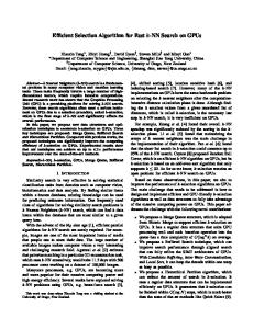
Figure 1. Implementation of three queue structures when k = 7. The solid lines with arrowheads represent an increasing order of values and the dashed lines with arrowheads represent position movement of elements. An example of inserting 3 into each queue is given to show how the elements are moved within each queue.

the following sections, we propose Merge Queue, Buffered Search, and Hierarchical Partition respectively. B. Queue Structures Traditionally there are two typical queues, insertion queue and heap queue [10]. The former maintains a sorted queue while the later maintains a maximum heap. As illustrated in the top of Fig. 1a, an element is inserted into the right position of insertion queue and all those larger elements move one position forward. The invariant of insertion queue is that the elements in the queue is fully ordered. Its average time complexity is O(k). In a heap queue, all elements are organized in a balanced binary tree. As illustrated in the bottom of Fig. 1a, its invariant is that a parent node should be larger than its child nodes. During insertion, elements move up and down in the tree to maintain the invariant. The average time complexity for inserting an element into heap queue is O(log k). The insertion queue is very regular and can be easily implemented on GPU. However, it suffers from a high time complexity. The heap queue has lower time complexity for each insertion. However, its tree structure requires a lot irregular memory accesses, since threads within one warp may enter different tree branches.

Algorithm 2: Insertion into Merge Queue (MQ insert). Input: dist, id : the element to be inserted; Input: dqueue, iqueue: the queue for storing k-NN; Input: k: the number of nearest neighbors required; Input: m: the size of the first and second levels. 1 flat insert(dist, id , dqueue, iqueue, m); 2 volatile shared int flag; 3 for (prev = 0, next = m; next < k; next× = 2) do 4 f lag = 0; 5 if dqueue[prev ] ≥ dqueue[next] then 6 flag = 1; 7 if flag == 0 then 8 return; 9 merge(dqueue, iqueue, 0, 2 × next); 10 prev = next;

C. Merge Queue To overcome the above limitations, we propose the following Merge Queue structure. Merge Queue is also organized in multiple levels, as shown in Fig. 1b. The size of the first and second levels is m, the size of the following levels is m × 2l−2 , where l > 2 and m could be 2i , i = 0, 1, 2, . . . . The invariant of Merge Queue is that, the elements of each level are sorted in a decreasing order so that the leftmost element (called Level Head) is the largest of that level, and the level heads are also sorted in decreasing order from top to bottom. This invariant guarantees that the first element (e.g. 7 in Fig. 1b) is the largest in the queue. In Merge Queue, the first level is maintained by insertion sort. A new element is always inserted to the first level and pushes out the largest element of the level. If the invariant is not satisfied after insertion, i.e., the head of the first level is smaller than that of the second level, a merge operation is applied to sort all elements in both levels so that the invariant is satisfied again. The merge operation is repeated if necessary at lower levels until the invariant is satisfied, i.e. all the level heads are in decreasing order. Since merge is not efficient when the size of the levels is too small, we can enlarge m, which is the size of the first and the second level, to avoid unnecessary merge operation. Unlike insertion queue and heap queue, merge queue allows Lazy Update which enables inserted elements to stay at upper levels as long as possible. For example, as Fig. 1b shows, in the Merge Queue on the right, after 3 is inserted, 7 is pushed out, and 6 becomes the largest at the first level. Since 6 is still larger than 5 (the head of the second level), it satisfies the invariant, and further merge operations are not needed. In contrast, insertion queue and heap queue would involve more data updates in such a situation, as shown in Fig. 1a. To complete the story, suppose a new element 4 (a duplicate) is inserted in the previous situation. It will push 6 out and become the head of level one. Since 4 is

0 2

4 6

7

5

3 1

6 4

2 0

7

5

3 1

7

5

4 6

0

2

3 1

6

4

5 7

0

2

3 1

7

6

4 5

3

2

0 1

6 7

5 4

3

2

0 1

6

5 4

3

2

1 0

7

5 4

3

2

1 0

7

(a) Original Bitonic Merge.

6

(b) Reverse Bitonic Merge.

Figure 2. Bitonic Merge and Reverse Bitonic Merge. Compared with the original method, the Reverse Bitonic Merge supports merging two sequences that are sorted in the same (decreasing) order. This makes it possible to merge elements from different levels of the Merge Queue.

smaller than 5 (the head of level two), merge operation will be required and the two levels will become (5, 4) and (4, 3). In summary, the advantage of Merge Queue is that it reduces data updates. Additionally it is possible to achieve better parallelism since the merge operation can be better parallelized on GPU. The pseudocode for Merge Queue is given in Algorithm 2. The merge operation is used to merge two sorted lists in the algorithm. We choose Bitonic Merge for merging two sorted lists since it has been proved to be very efficient on GPU [17]. As Fig. 2a shows, there are two lists of elements. One is sorted in increasing order and the other is in decreasing order, which form a Bitonic Sequence. Given a bitonic sequence, the Bitonic Sorting Network can merge it efficiently, as shown in Fig. 2a. Assume l is the size of the bitonic sequence, the sorting network can merge the two lists by using a fixed number of compare-and-swap operations ( 2l ) in a fixed number of steps (log l). Thus, Bitonic Merge has a time complexity of O( 2l log l). Since the original Bitonic Merge only supports merging two lists sorted in opposite order and our Merge Queue requires to merge two lists sorted in the same order, we propose a Reverse Bitonic Merge. As shown in Fig. 2b, compared with the original merge, the Bitonic Sorting Network in the dashed box is changed slightly, so that the elements are cross-compared and exchanged if needed. In this way, the two lists sorted in the same decreasing order in Merge Queue can be efficiently merged on GPU. To merge a bitonic sequence sized l, it takes O( 2l log l). However, due to Lazy Update, only when the head of an upper level is smaller than the head of the lower level will a merge be required. For example, when the last level is to be merged in Merge Queue of size k, at least k4 (the size of the second last level) new elements have to be inserted into the second last level. Otherwise, the level head of the second last level is still smaller than that of the last level and the merge

Queue

List

𝑞0

4

6

7 3 5 1

𝑞1

4

2

5 6 0 3

𝑞2

5

6 4 6 3 1

Buffer

Filled Buffer

Sorted Buffer

① Aligned Search

② Intra-warp Communication

③ Local Sort

Figure 3. Improve the SIMT efficiency through the use of a buffer. To illustrate, we use three queries with k = 4 as an example. The shaded numbers are those to be inserted to the queue.

operation is not needed. Thus, the average time complexity k log k per insert is O( 2 k ) = O(2 log k). Since there are log k 4 levels in the queue and an insert may involve the merge of all levels in the worst case, the overall average time complexity log Pk is O( 2 log 2ki ) = O(log2 k + log k) = O(log2 k). i=0

Aligned Merge in Merge Queue: In Merge Queue, a merge operation is called when a thread finds out that the invariant of its queue is not satisfied. Since different threads within a warp will do merge operations at different times, it causes many branches and thus poor SIMT efficiency. We use a technique called Intra-Warp Communication to synchronize the merge operation among different threads of the same warp (line 4-8 in Algorithm 2). We set a flag in the shared memory that is visible to all threads within one warp. If any thread finds that a merge is needed in its queue, it will set the flag to inform other threads that it is time to merge. Since threads do merge together, it reduces the number of branches due to merge, although it may bring some extra work to some otherwise idle threads. D. Buffered Search In k-selection, k is usually much smaller than the number of references N . Since most of the references are going to be ignored, k-selection may meet significant thread divergence due to frequent branches. Take Fig. 3 as an example. Suppose there are three k-NN queries executed by three threads in parallel and k = 4. For each query, there is a list of references (elements) to be searched. According to the current scenario, some elements (shaded gray) need to be inserted into the queue as their values are smaller than the largest value in the queue, while other elements do not. While any of the shaded elements is inserted, all other threads have to be idle due to SIMT. For example, when 4 is inserted into the queue of q0 , threads working on q1 and q2 are idle, which results in poor utilization of GPU cores. To solve this problem, we propose Buffered Search. Its pseudocode is in Algorithm 3. During k-NN search, the list is checked and the k-NN candidates are put into the buffer first (line 4-7). Then, these candidates in the buffer will be inserted into the queue (line 12) if any of the buffers is full.

Algorithm 3: Buffered search. Input: dlist, ilist: list of elements to be searched; Input: dbuffer , ibuffer : buffer for storing candidates; Input: dqueue, iqueue: the queue for storing k-NN; Input: bsize: buffer size. 1 volatile shared int flag = 0; 2 int cur = 0; 3 forall the dist, id ∈ dlist, ilist do 4 if dist < queue[0] then 5 dbuffer [cur ] = dist; 6 ibuffer [cur ] = id; 7 cur ++; 8 if cur == bsize then 9 flag = 1; 10 if flag == 1 then 11 sort the elements in the buffer; 12 insert elements from the buffer into the queue; 13 cur = flag = 0;

To check if the buffer of a thread is full, we again use the Intra-warp Communication technique. We set a flag variable in the shared memory for each warp (line 1). Each time an element is added into the buffer, the thread will check whether its buffer is full. If any thread’s buffer is full within the warp, the flag is set to 1 (line 8-9). All other threads will be informed through this flag and start inserting elements from the buffer into the queue (line 10-13). In this way, the number of branches is reduced and better SIMT efficiency can be achieved. When the buffer is full, we sort the elements in the buffer, which is called Local Sort (line 11). Since the buffer is quite small, sorting the buffer will bring little overhead but does provide benefits. When the elements in the buffer are sorted in increasing order, the smallest element will be inserted to the queue first. Then, when larger elements is inserted later, some of them will no longer need to be inserted due to a smaller queue head. Therefore, better performance can be achieved especially when k is large and insertion is expensive.

Pick 0

3 4 4

6

4 10 14 Figure 4.

5 6 11 5 3

3, 0

2

3 3

8 7 8

13 2

0 2

0 15 9

4, 3, 2, 0 1

0 12 1

8, 2, 0, 1 9, 0, 12, 1

Hierarchical partition (N = 16, k = 2 and G = 2). The structure is built in bottom-up while searched in top-down direction.

E. Hierarchical Partition Since N is usually very large and k is relatively small, we propose the Hierarchical Partition algorithm to reduce the number of elements that need to be searched. Fig. 4 shows an example of Hierarchical Partition with a group size G = 2, assuming N = 16 and k = 2. In Hierarchical Partition, we divide the list of elements to be searched into small groups. Then, we search for the smallest elements within each group and use them to form a new list. This procedure is repeated until there are no more than k elements in the new list. To build up this structure, its pseudocode, called Bottom-Up Construction, is given in Algorithm 4. Construction of the hierarchical structure takes a linear scan of the whole list (N elements). So it takes O(N ) time to create the second list, which has N G elements. This procedure is repeated until the current list has fewer than k elements. Thus, the time complexity for building this structure takes logP GN N N G−1 O( Gi ) = O( G−1 ) = O(N ). It costs an extra space i=0

Queue

G−1 of O( NG−1 −N ) = O(N ) (excluding the space taken by the original list). The construction can be done very efficiently on GPU since all the memory accesses are coalesced and all threads can work on their own list in perfect SIMT style. During k-NN search, we go in the opposite direction, which is called Top-Down search. We first insert all the elements of the top list into the queue. Then we pick the elements that belong to the sub-groups of those current candidate k-NNs and insert them into the queue. This procedure is repeated until the bottom list is reached. Note that, when we insert an element into the queue, its index in the list is also inserted as well. If the index of an element is i in the current list, the elements of its sub-group are in the range of [iG, (i + 1)G) in the lower list, where G is size of group. If any element in the upper level does not belong to k-NN, none of the elements in its sub-groups would belong to k-NN since all of them are larger than the lead element. In this way, it guarantees that the k smallest elements will be contained in the queue. Due to space limitation, we do not give the pseudocode for the Top-Down search. During Top-Down search, Hierarchical Partition will pick at most Gk candidate elements at each level of the structure and there are at most (logG N − logG k) levels that need to

Algorithm 4: Bottom-Up Construction Input: dlist: list of elements to be searched; Input: N : size of the dlist; Input: levels[][]: the structure for storing each level in the hierarchical structure; Input: G: number of elements within each sub-group; Input: k: number of nearest neighbors required. 1 2 3 4 5 6 7 8 9 10 11 12 13 14 15 16 17 18 19

levels[0] = dlist; cur size = N; cur level = 0; while cur size > k do next size = d N / G e; next level = cur level + 1; initialize levels[next level ] with next size; cur = 0; min = ∞; while cur < cur size do if levels[cur level ][cur ] < min then min = levels[cur level ][cur ]; cur ++; if cur %G == 0 then levels[next level ][cur /G - 1] = min; min = ∞; levels[next level ][cur /G] = min; cur level ++; cur size = next size;

be searched. Thus, search with Hierarchical Partition can be N finished within logG N k steps and only Gk logG k elements will be picked for insertion. Compared with searching the N whole list, the speedup is roughly Gk log N . G k Compared with the other partition-based algorithms like Quick Select [9], Bucket or Radix Select [12], Hierarchical Partition can finish searching within fixed steps. Compared with those Divide-and-Merge methods [7], [13], [14], our method avoids sorting the elements within each group. Its performance is expected to increase when N is increasing. However, when k is increasing, the performance will decrease. In our experiments, we have tested a range of k up to 1024 which is large enough for most k-NN applications.

A. Merge Queue When many elements are inserted into a queue, the values at different positions of the queue will be updated for

600

Insertion Queue Heap Queue Merge Queue

500

Updates

In this section, we evaluate our proposed methods on a GPU using a synthetic data set. The query and reference tuples of k-NN used in the following experiments are randomly generated. Each tuple has a dimensionality of 128 with each value distributed in the range of [0, 1]. The method of [3] is used to calculate their distances and store them as a matrix in the GPU global memory while our selection algorithms are used to find the k-NN of each query. In all experiments, we report performance results with N ∈ [213 , 216 ] and k ∈ [25 , 210 ] to show the scalability of our methods as N and k increase. The number of queries Q is set to 213 to generate a sufficient number of threads on the GPU since each thread can process one query in our algorithm. The range of N covers a wide variety of problem sizes. A divide-and-merge method [18] can be applied to support N larger than the range without hurting the performance, although this is out of scope of this paper. The range of k is chosen because it is used in other related work [6], [9], [13], and we believe that it is large enough to cover a wide range of k-NN applications. When k is smaller than 25 , k-selection is less challenging than distance calculation on GPU and thus is less worth discussion in this paper. For the merge queue, we set m = 8 since we find that experimentally this configuration can maximize its performance. Although many approximate k-NN algorithms are quite sensitive to the data set [19], k-selection is oblivious to them since the distance values have already been computed so that they are accurate and we can assume the k-NNs are randomly distributed in each list of the distance values. Since experimental results on different data sets are similar, to save space, we only give the results on the synthetic data set here. All experiments were run on the NVIDIA Tesla C2075 Fermi GPU with 14 SMs and 448 cores at 1.15GHz SM clock frequency, which can provide up to 515 Gflops double precision and 1.03 Tflops single precision floating point peak performance. It has a 6 GB GDDR5 memory with a 1.5 GHz DRAM clock frequency which can provide a bandwidth up to 144 GB/sec. The cache is configured to have 16 KB L1 cache and 48 KB shared memory. All source files are compiled with CUDA 5.5. To make a fair comparison, we also use a multicore machine which is equipped with two sockets of Intel Xeon E5-2665 CPUs. There are 16 cores in total with 8 cores in each CPU that run at 2.40 GHz frequency. It also gets a 20 MB last level cache that will benefit the k-selection a lot since the queue can fit in the cache. We use the heap algorithm from C++ standard library as the k-selection algorithm and parallelize it with OpenMP on CPU.

400 300

200 100 0

3000

Total Updates

IV. E VALUATION

Insertion Queue Heap Queue Merge Queue

2500 2000 1500 1000 500 0

0

10

20 30 40 50 60 Position in the queue

(a) Updates per Position

70

5

6

7

8

9

10

log k

(b) Total updates

Figure 5. Number of updates in the three types of queues during kselection. Here, N = 215 . In (a), we show the updates happened at each position of a queue, when k = 26 . In (b), we show the total number of updates of each queue when k is increasing (k ∈ [25 , 210 ]).

different times due to data movement. In general, the head of a queue is updated most frequently since it contains the largest value that keeps changing. The tail of a queue is updated less frequently since the smallest element is kept at the tail, which is more stable during insertion operation. Fig. 5 shows the number of updates during k-selection when the three types of queues are used. For the insertion queue, the number of updates decreases linearly towards the tail of the queue. This is because each time when an element is inserted, all those larger elements in the queue will move one step forward to the head. For the heap queue, the number of updates depend on the level which the position is on. Usually the last level of the heap (positions close to the tail) has the least number of updates. Merge queue has a similar behavior to heap queue except the number of updates at each position is slightly larger. When most of the updates happen close to the head, better locality can be achieved. As Fig. 5b shows, the total number of updates in insertion queue increases dramatically when k is increasing. Both heap queue and merge queue perform much better, as their total numbers of updates increase much slower when k is increasing, although merge queue performs slightly worse than heap queue. This results match our previous analysis on time complexity that each insertion operation takes O(k) for insertion queue, O(log k) for heap queue, and O(log2 k) for merge queue. B. Buffered Search original running time The performance improvement ( optimized running time ) after applying Buffered Search to each queue is shown in Fig. 6. As we can find, using a full buffer through intrawarp communication is always better than using buffer only. Sorting the buffer suits insertion queue better than heap and merge queue. Buffered search achieves the best performance improvement when k = 28 , but the improvement decreases when k is increasing. The highest improvements are 5.39×, 1.28× and 1.85× for the three types of queue respectively. By comparing the three queues, we find the improvement for the insertion queue is the best. This is because insertion queue has the highest time complexity that its performance

6

buffer

full

1.5

full+sorted

buffer

full

2

full+sorted

4 3 2

Improvement

Improvement

Improvement

5 1

0.5

1 0 7

8

9

5

6

7

log k

G=4

G=6

G=8

9

10

5

6

7

8

9

10

9

10

log k

(b) Heap queue.

4

Improvement

Improvement

8

G=2

8

(c) Merge queue.

Performance improvement of buffered search with an increasing value of k. Here, N = 215 .

Figure 6.

6 4

G=2 G=6

8

G=4 G=8

7

3

2

G=2

G=4

G=6

G=8

6

5 4 3

2

1 5

6

7

log k

8

9

2

10

5

6

(a) Insertion queue

G=2 G=6

9

10

4

G=4 G=8

6 4 2 14

log N

15

6

G=2 G=6

3.5

16

(a) Insertion queue Figure 8.

7

log k

8

(c) Merge queue 215 .

7

G=4 G=8

3 2.5 2

13

5

Scalability of Hierarchical Partition with increasing k. Here, N =

Improvement

8

log k

8

Improvement

10

7

(b) Heap queue

Figure 7.

Improvement

0.5

log k

(a) Insertion queue.

10

full+sorted

0

10

Improvement

6

full

1

0 5

buffer

1.5

G=2 G=6

6

G=4 G=8

5 4 3 2

13

14

log N

15

16

13

(b) Heap queue Scalability of Hierarchical Partition with increasing N . Here, k =

14

log N

15

16

(c) Merge queue 28 .

will be significantly influenced when there are too many branches that can lead to poor SIMT efficiency. When some threads are working while others are idle in the same warp, the idle threads have to wait longer due to the longer insertion time. For heap queue, it achieves less improvement since each insertion takes less time. Similarly, due to Lazy Update in merge queue, its performance improvement is not as much as insertion queue, but is still quite significant especially when k is smaller.

with a fixed N = 215 is 7.4×, 3.4×, 5.69× for insertion queue, heap queue and merge queue, respectively. As shown in Fig. 8, for a fixed k = 28 , the peak improvement is 8.94×, 3.0× and 6.23× for the three queues, respectively. As discussed previously, the performance improvement will increase with increasing N and decrease with increasing k. This is because when N is increasing more elements can be excluded. On the contrary, when k is increasing, elements will have more chances to be picked during top-down search.

C. Hierarchical Partition Fig. 7 and 8 show the scalability of Hierarchical Partition with increasing k and N . Notice that, the time for constructing the tree structure is already contained in the figures. We find this method is effective in improving the performance of the three queues. According to Fig. 7, the peak improvement

From the figures, we can also find an optimal value for G, which is the size of the group in the Hierarchical Partition. A smaller G (e.g. 2) costs more memory to store the hierarchical structure, while a larger G (e.g. 8) reduces memory cost but performance improvement diminishes. In the following sections, we choose G = 4 by default since

Table I E XECUTION TIME ( SEC .) OF k- SELECTION ALGORITHMS .

``` `` k & N Algorithms ```` Distance Calculation on GPU Data Copy CPU-based CPU 1 CPU 16 Insertion Queue GPU-based (original) Heap Queue Merge Queue Merge Queue aligned Insertion Queue buf+hp GPU-based (optimized) Heap Queue buf+hp Merge Queue buf+hp Merge Queue aligned+buf+hp Truncated Bitonic Sort State-of-the-art Quick Multi-Select

5 0.14 0.46 0.34 0.03 0.12 0.05 0.13 0.07 0.04 0.04 0.04 0.04 0.30 -

it only costs N3 extra memory for each query but its performance improvement is the best in most cases. D. Overall Performance Fig. 9 shows the overall performance improvement when both Buffered Search and Hierarchical Partition are applied to the queues. These methods achieve the largest improvement on insertion queue, with a peak improvement of 14.83× at k = 28 in Fig. 9a and a peak improvement of 16.89× at N = 216 in Fig. 9b. The improvements for heap queue and merge queue are smaller but they are significant enough (between 1.25× and 3.57× for heap queue, between 3.25× and 7.49× for merge queue). Table I gives the execution times of different k-selection algorithms. The time cost on calculating the distance values on GPU is given as a baseline (“Distance Calculation on GPU”). For a fixed N , the time spent on distance calculation is the same (0.14 sec.). When N is increasing, its time will increase slightly. However, when k is increasing, the time cost on k-selection will increase much faster. In most cases, the time cost on k-selection is much larger than that of distance calculation. This proves that k-selection is a major bottleneck in k-NN search.

20

Insertion_buf+hp heap_buf+hp Merge_buf+hp

15

Improvement

Improvement

20

10 5 0

15

Insertion_buf+hp heap_buf+hp Merge_buf+hp

10 5 0

5

6

7

log k

8

9

10

(a) k ∈ [25 , 210 ], N = 215

13

14

log N

15

16

(b) N ∈ [213 , 216 ], k = 28

Figure 9. Performance improvement after applying both Buffered Search and Hierarchical Partition on each queue.

6 0.14 0.46 0.46 0.05 0.37 0.09 0.33 0.1 0.05 0.05 0.07 0.05 0.36 0.21

log k (N = 215 ) 7 8 9 0.14 0.14 0.14 0.46 0.46 0.46 0.68 1.1 1.9 0.07 0.2 0.19 1.16 3.56 10.44 0.19 0.41 0.85 0.89 2.24 5.29 0.16 0.29 0.57 0.1 0.24 0.71 0.08 0.15 0.31 0.13 0.39 0.82 0.08 0.14 0.27 0.44 0.53 0.64 0.22 0.22 0.23

10 0.14 0.46 3.45 0.42 29.03 1.71 11.57 1.1 2.58 0.74 2.77 0.58 -

13 0.03 0.13 0.72 0.06 1.83 0.27 1.49 0.18 0.2 0.11 0.35 0.1 0.13 0.15

log N (k = 28 ) 14 15 0.07 0.14 0.25 0.49 0.87 1.08 0.07 0.08 2.62 3.53 0.33 0.4 1.85 2.22 0.23 0.29 0.21 0.24 0.12 0.15 0.29 0.4 0.11 0.14 0.26 0.53 0.18 0.22

16 0.28 0.99 1.43 0.11 4.56 0.48 2.62 0.38 0.27 0.17 0.35 0.17 1.04 0.30

In Table I, we also give the results of k-selection with multicore CPU (“CPU-based”). CPU 1 represents its serial performance and CPU 16 represents its parallel performance when 16 threads are used. As we can find, compared with the time cost by k-selection on GPU, parallel k-selection on CPU achieves a good performance. However, if the overhead of data movement from GPU memory to the main memory (“Data Copy”) is considered, it significantly overshadows the benefit of doing k-selection on CPU side. To demonstrate the performance of doing k-selection on the GPU side, we report the results of using aforementioned three queues (“GPU-based”). For the un-aligned merge queue, it performs better than insertion queue but much worse than heap queue. However, when we use aligned merge, its performance can be improved by up to 10.51×. This result shows the importance of improving SIMT efficiency on GPU. The performance improvement after applying Buffered Search and Hierarchical Partition is consistent with our previous results. Our optimized merge queue (“Merge Queue aligned+buf+hp”) is the best among all implementations of k-selection on GPU, which is 1.3× better than the second best (“Heap Queue buf+hp”) when k = 210 and N = 215 . We also make a comparison with two recent works (“State-of-the-art”): Truncated Bitonic Sort (TBS) [13] and Quick Multi-Select (QMS) [9]. TBS’s source code is publicly available. However, we find that it only supports k ≤ 512. Since we do not have QMS’s source code, we pick some of the timing results from their paper [9]. Notice that, the results for QMS was run on NVIDIA Tesla C2050, which has a similar configuration as our C2075, except that it only has 3 GB of global memory. It also uses CUDA 4.2 to compile the source code, which is different from our CUDA 5.5. As we can find, our optimized heap and merge queue are very competitive compared with state-of-the-art methods.

They can beat TBS by 2.37× to 7.5× while beat QMS up to 4.2× when k is small. It is worth noting that, QMS does not return sorted k-NN (the results contain all the k-NN, but are not sorted in order). If this is considered, sorting the results will cost extra time, especially when k is large. Meanwhile, QMS performs worse when N is increasing while the time of ours increases much slower. V. C ONCLUSION In this paper, we propose three key techniques named Merge Queue, Buffered Search and Hierarchical Partition to accelerate k-selection on GPU. Merge Queue provides efficient partially-sorted queue on GPU, Buffered Search improves SIMT efficiency, and Hierarchical Partition reduces the number of elements searched in k-selection. Experimental results show that our proposed techniques are efficient and achieve up to 4.2× better performance than the stateof-the-art works. In the future, we could improve our Merge Queue by using more efficient merge algorithms on GPU, e.g. Adaptive Bitonic Merge [17] and Merge Path [20]. We also plan to test the proposed techniques on other accelerators such as the Intel Xeon Phi that have Vector Processing Units. ACKNOWLEDGMENT The authors thank the anonymous reviewers for their valuable comments. This work is partially sponsored by the National Basic Research 973 Program of China (No. 2015CB352403), the National Natural Science Foundation of China (NSFC) (No. 61261160502, No. 61272099), the Program for Changjiang Scholars and Innovative Research Team in University (IRT1158, PCSIRT), the Scientific Innovation Act of STCSM (No. 13511504200), and the EU FP7 CLIMBER project (No. PIRSES-GA-2012-318939). R EFERENCES [1] J. Manyika, M. Chui, B. Brown, J. Bughin, R. Dobbs, C. Roxburgh, and A. H. Byers, “Big data: The next frontier for innovation, competition, and productivity,” McKinsey Global Institute, Tech. Rep., 2011. [2] S. Agarwal, Y. Furukawa, N. Snavely, I. Simon, B. Curless, S. M. Seitz, and R. Szeliski, “Building Rome in a day,” Communications of the ACM, vol. 54, no. 10, pp. 105–112, 2011. [3] V. Garcia, E. Debreuve, F. Nielsen, and M. Barlaud, “Knearest neighbor search: Fast GPU-based implementations and application to high-dimensional feature matching,” in Image Processing (ICIP), 2010 17th IEEE International Conference on, 2010, pp. 3757–3760. [4] Q. Kuang and L. Zhao, “A practical GPU based kNN algorithm,” in International symposium on computer science and computational technology (ISCSCT), 2009, pp. 151–155. [5] S. Li, L. Simons, J. B. Pakaravoor, F. Abbasinejad, J. D. Owens, and N. Amenta, “kANN on the GPU with shifted sorting,” in Proceedings of the Fourth ACM SIGGRAPH / Eurographics Conference on High-Performance Graphics, ser. EGGH-HPG’12. Aire-la-Ville, Switzerland, Switzerland: Eurographics Association, 2012, pp. 39–47.

[6] J. Pan and D. Manocha, “Fast GPU-based locality sensitive hashing for k-nearest neighbor computation,” in Proceedings of the 19th ACM SIGSPATIAL International Conference on Advances in Geographic Information Systems, ser. GIS ’11. New York, NY, USA: ACM, 2011, pp. 211–220. [7] R. Barrientos, J. Gmez, C. Tenllado, M. Matias, and M. Marin, “kNN query processing in metric spaces using GPUs,” in Euro-Par 2011 Parallel Processing, ser. Lecture Notes in Computer Science, E. Jeannot, R. Namyst, and J. Roman, Eds. Springer Berlin Heidelberg, 2011, vol. 6852, pp. 380–392. [8] L. Cayton, “Accelerating nearest neighbour search on manycore systems,” in IEEE Int. Parallel and Distributed Processing Symposium (IPDPS), 2012. [9] I. Komarov, A. Dashti, and R. D’Souza, “Fast k-NNG construction with GPU-based quick multi-select,” PLoS ONE 9(5): e92409, 2014. [10] T. H. Cormen, C. E. Leiserson, R. L. Rivest, and C. Stein, Introduction to algorithms. MIT press Cambridge, 2001. [11] L. Monroe, J. Wendelberger, and S. Michalak, “Randomized selection on the GPU,” in Proceedings of the ACM SIGGRAPH Symposium on High Performance Graphics, ser. HPG ’11. New York, NY, USA: ACM, 2011, pp. 89–98. [12] T. Alabi, J. D. Blanchard, B. Gordon, and R. Steinbach, “Fast k-selection algorithms for graphics processing units,” J. Exp. Algorithmics, vol. 17, pp. 4.2:4.1–4.2:4.29, Oct. 2012. [13] N. Sismanis, N. Pitsianis, and X. Sun, “Parallel search of k-nearest neighbors with synchronous operations,” in High Performance Extreme Computing (HPEC), 2012 IEEE Conference on, Sept 2012, pp. 1–6. [14] L. Jian, C. Wang, Y. Liu, S. Liang, W. Yi, and Y. Shi, “Parallel data mining techniques on graphics processing unit with compute unified device architecture (CUDA),” The Journal of Supercomputing, vol. 64, no. 3, pp. 942–967, 2013. [15] N. Satish, M. Harris, and M. Garland, “Designing efficient sorting algorithms for manycore GPUs,” in Parallel Distributed Processing, 2009. IPDPS 2009. IEEE International Symposium on, May 2009, pp. 1–10. [16] N. Leischner, V. Osipov, and P. Sanders, “GPU sample sort,” in Parallel Distributed Processing (IPDPS), 2010 IEEE International Symposium on, April 2010, pp. 1–10. [17] H. Peters, O. Schulz-Hildebrandt, and N. Luttenberger, “A novel sorting algorithm for many-core architectures based on adaptive bitonic sort,” in Proceedings of the 2012 IEEE 26th International Parallel and Distributed Processing Symposium, ser. IPDPS ’12. Washington, DC, USA: IEEE Computer Society, 2012, pp. 227–237. [18] A. S. Arefin, C. Riveros, R. Berretta, and P. Moscato, “Gpufs-knn: A software tool for fast and scalable knn computation using gpus,” PloS one, vol. 7, no. 8, p. e44000, 2012. [19] X. Tang, S. Mills, D. Eyers, K.-C. Leung, Z. Huang, and M. Guo, “Data filtering for scalable high-dimensional k-nn search on multicore systems,” in Proceedings of the 23rd International Symposium on High-performance Parallel and Distributed Computing, ser. HPDC ’14. New York, NY, USA: ACM, 2014, pp. 305–310. [20] O. Green, R. McColl, and D. A. Bader, “GPU merge path: a GPU merging algorithm,” in Proceedings of the 26th ACM international conference on Supercomputing, ser. ICS ’12. New York, NY, USA: ACM, 2012, pp. 331–340.