Master project report
DynaProg for Scala A Scala DSL for Dynamic Programming on CPU and GPU
Laboratory Professor Supervisors Expert Student Semester
Programming Methods Laboratory, LAMP, EPFL Martin Odersky Vojin Jovanovic, Manohar Jonnalagedda Mirco Dotta, Typesafe Thierry Coppey Autumn 2012
DynaProg for Scala, p. 1
Abstract Dynamic programming is an algorithmic technique to solve problems that follow the Bellman’s principle[3]: optimal solutions depends on optimal sub-problem solutions. The core idea behind dynamic programming is to memoize intermediate results into matrices to avoid multiple computations. Solving a dynamic programming problem consists of two phases: filling one or more matrices with intermediate solutions for sub-problems and recomposing how the final result was constructed (backtracking). In textbooks, problems are usually described in terms of recurrence relations between matrices elements. Expressing dynamic programming problems in terms of recursive formulae involving matrix indices might be difficult, if often error prone, and the notation does not capture the essence of the underlying problem (for example aligning two sequences). Moreover, writing correct and efficient parallel implementation requires different competencies and often a significant amount of time. In this project, we present DynaProg, a language embedded in Scala (DSL) to address dynamic programming problems on heterogeneous platforms. DynaProg allows the programmer to write concise programs based on ADP [15], using a pair of parsing grammar and algebra; these program can then be executed either on CPU or on GPU. We evaluate the performance of our implementation against existing work and our own hand-optimized baseline implementations for both the CPU and GPU versions. Experimental results show that plain Scala has a large overhead and is recommended to be used with small sequences (≤ 1024) whereas the generated GPU version is comparable with existing implementations: matrix chain multiplication has the same performance as our hand-optimized version (142% of the execution time of [39]) for a sequence of 4096 matrices, Smith-Waterman is twice slower than [13] on a pair of sequences of 6144 elements, and RNA folding is on par with [31] (95% running time) for sequences of 4096 elements.
Acknowledgement This project has been achieved in collaboration with Manohar Jonnalagedda. I also would like to thank the LAMP team, including Eugene Burmako, Sandro Stucki, Vojin Jovanovic and Tiark Rompf who provided insightful advices and suggestions.
CONTENTS
DynaProg for Scala, p. 2
Contents 1 Introduction
4
2 Background
6
2.1
Graphic cards . . . . . . . . . . . . . . . . . . . . . . . . . . . . . . . . . . . . . .
6
2.2
ADP and parsing grammars . . . . . . . . . . . . . . . . . . . . . . . . . . . . . .
7
2.3
Scala . . . . . . . . . . . . . . . . . . . . . . . . . . . . . . . . . . . . . . . . . . .
10
2.4
Lightweight Modular Staging . . . . . . . . . . . . . . . . . . . . . . . . . . . . .
10
2.5
Related work . . . . . . . . . . . . . . . . . . . . . . . . . . . . . . . . . . . . . .
11
3 Dynamic programming problems
12
3.1
Problems classification . . . . . . . . . . . . . . . . . . . . . . . . . . . . . . . . .
12
3.2
Problems of interest . . . . . . . . . . . . . . . . . . . . . . . . . . . . . . . . . .
14
3.3
Related problems . . . . . . . . . . . . . . . . . . . . . . . . . . . . . . . . . . . .
24
4 Architecture design and technical decisions
26
4.1
User facing language requirements . . . . . . . . . . . . . . . . . . . . . . . . . .
26
4.2
Recurrences analysis . . . . . . . . . . . . . . . . . . . . . . . . . . . . . . . . . .
28
4.3
Backtracking . . . . . . . . . . . . . . . . . . . . . . . . . . . . . . . . . . . . . .
30
4.4
CUDA storage: from list to optional value . . . . . . . . . . . . . . . . . . . . . .
33
4.5
Memory constraints . . . . . . . . . . . . . . . . . . . . . . . . . . . . . . . . . .
34
4.6
Memory layout . . . . . . . . . . . . . . . . . . . . . . . . . . . . . . . . . . . . .
38
4.7
LMS integration . . . . . . . . . . . . . . . . . . . . . . . . . . . . . . . . . . . .
39
4.8
Compilation stack . . . . . . . . . . . . . . . . . . . . . . . . . . . . . . . . . . .
40
5 Implementation
42
5.1
CUDA baseline . . . . . . . . . . . . . . . . . . . . . . . . . . . . . . . . . . . . .
42
5.2
Scala parsers . . . . . . . . . . . . . . . . . . . . . . . . . . . . . . . . . . . . . .
44
5.3
Code generation . . . . . . . . . . . . . . . . . . . . . . . . . . . . . . . . . . . .
46
5.4
Runtime execution engine . . . . . . . . . . . . . . . . . . . . . . . . . . . . . . .
50
5.5
LibRNA . . . . . . . . . . . . . . . . . . . . . . . . . . . . . . . . . . . . . . . . .
51
6 Usage
52
6.1
Program examples . . . . . . . . . . . . . . . . . . . . . . . . . . . . . . . . . . .
52
6.2
Other usage options . . . . . . . . . . . . . . . . . . . . . . . . . . . . . . . . . .
57
7 Benchmarks
57
7.1
Metrics . . . . . . . . . . . . . . . . . . . . . . . . . . . . . . . . . . . . . . . . .
57
7.2
Benchmarking platform . . . . . . . . . . . . . . . . . . . . . . . . . . . . . . . .
58
CONTENTS
DynaProg for Scala, p. 3
7.3
Matrix chain multiplication . . . . . . . . . . . . . . . . . . . . . . . . . . . . . .
59
7.4
Smith-Waterman (affine gap cost)
. . . . . . . . . . . . . . . . . . . . . . . . . .
60
7.5
Zuker RNA folding . . . . . . . . . . . . . . . . . . . . . . . . . . . . . . . . . . .
62
7.6
Synthetic results . . . . . . . . . . . . . . . . . . . . . . . . . . . . . . . . . . . .
63
8 Future work
63
9 Conclusion
66
1
INTRODUCTION
DynaProg for Scala, p. 4
1 Introduction Dynamic programming (DP) is an algorithmic technique to solve optimization problems. For example, we might want to multiply a chain of matrices1 efficiently. The order in which matrices are combined changes the number of required scalar multiplications, therefore we would want to find an optimal order that minimizes this number. Notice that if we know how to split the chain into two subparts, we can recursively find an optimal order in these two parts and recombine them. Such combinatorial problems verify the Bellman’s principle[3]: «optimal solutions depends on optimal solutions of sub-problems»2 . In order to find the optimal way of splitting the chain, we would need to explore an exponential number of possibilities. Using the Bellman’s principle, we can memorize intermediate optimal solutions to save redundant computations, thereby reducing the problem to a polynomial complexity. Dynamic programming problems are usually expressed in terms of recurrences on intermediate solutions that are stored in matrices, whereas optimality is defined in terms of an objective function (minimal or maximal cost, ...). In the case of a chain of n matrices, the recurrence is: M(i,i) = 0
∧
M(i,j) =
min
1≤i≤k
{M(i,k) + M(k+1,j) + ri · ck · cj }
∀1 ≤ i, j ≤ n
where ri and ci denotes respectively the row and column of the ith matrix in the chain, M is an n × n matrix and M(i,j) stores the number of multiplications to obtain the product of matrices in the chain i, ..., j. The total number of required scalar multiplications is given by M(1,n) (refer to §3.2.5 for details). Once the optimal result is found, a second backtrack phase retrieves the construction trace associated with the optimal score for the problem. This trace (or backtrack trace) describes how to obtain the optimal score, and heavily depends on the matrix design. In several disciplines of applied Computer Science, for example, biosequence analysis, natural language processing and operational research, dynamic programming problems such as sequence alignment, RNA sequence folding or expression parenthesisation could arise. Unfortunately, these often appear in multiple variations with a considerable degree of sophistication such that there is a mismatch between the textbook solution and its concrete implementation. The user is often interested in one optimal solution, but he might also request all co-optimal solutions, a fixed number of near-optimal solutions, or some synthetic properties of the search space (size, sum of scores, ...). The backtracking is usually ad-hoc because it needs to be kept consistent with matrix filling and presented in a format suitable for the user (readable by human or ready to drive further computations). Additionally, debugging matrix indices is tedious and requires a lot of time, and small changes in the formulae might imply large rewrites of the matrices and recurrences [17]. Finally, once the implementation is correct, it is possible to turn it into an efficient implementation for specific architectures such as multi-CPU, GPU and programmable hardware (FPGA). However, domain specialists who write the recurrences might not be very familiar with these platforms, and parallelization or hardware experts might not deeply understand the domain of the dynamic programming recurrences.
1 2
Such that matrices have appropriate dimensions to be multiplied with each other. http://en.wikipedia.org/wiki/Bellman_equation#Bellman.27s_Principle_of_Optimality
1
INTRODUCTION
DynaProg for Scala, p. 5
To simplify the expression of dynamic problems, Algebraic Dynamic Programming (ADP) [15] proposes a language-independent declarative approach that separates the concerns of dynamic programming on sequences into four distinct components that are tightly connected: 1. The search space is described by a context-free parsing grammar that produces intermediate solution candidates whose score might be inserted in the matrix. 2. Constructed candidates are then evaluated by a scoring function (where all these functions form an algebra), so that they can be compared appropriately. 3. The objective function (or aggregation function) operates on the scores previously obtained to retain valid candidates. 4. Finally, results are tabulated (memoized in an array) in corresponding matrices. Tabulation process regulates the trade-off between running time and space efficiency by memoizing appropriate results that are reused multiple times. A signature serves as interface between the grammar, the scoring algebra and the aggregation function, which allows the user to combine one grammar with different algebras or vice versa. Because recurrence relations are expressed by a parsing grammar, ADP makes the candidate structure explicit and hides tabulation indices, thereby preventing potential errors. Finally, since the expression of the dynamic program is formalized and abstracted into a grammar and an algebra, it becomes possible to systematically convert dynamic programming descriptions into efficient recurrences for many-core platforms such as GPUs [37]. DynaProg, the DSL we present in this report, implements the concepts of ADP in Scala as an embedded DSL (domain-specific language) with a syntax similar to the combinators parsers of Scala library3 . It extends ADP by allowing grammars for pairing two sequences (multi-track grammars) similarly as GAPC[35]. It also simplifies the process of writing programs by inferring additional information (§4.2.2). Moreover, it can translate them into efficient CUDA4 program that are competitive to their handwritten counterpart (§7). Since the program structure is formalized in ADP framework, it can be analyzed to remove unused grammar rules (§4.2.1) and avoid some non-termination issues; since it is generated, correct scheduling is guaranteed and indices errors are avoided, thereby it produces an arguably more reliable program. DynaProg provides a generic way of backtracking the results such that the same trace can be used with different algebras sharing the same grammar. This allows constructing a two step pattern to solve problems: first the DP problem is solved using the appropriate cost functions; then from the backtrack of its optimum, the desired result is computed. As example, consider multiplying a chain5 of matrices efficiently: first, optimal execution scheduling (or parenthesisation) trace is found using dynamic programming and cost algebra (§3.2.5). The backtrack trace is then used (with a multiplication algebra) to multiply the actual matrices. Finally, offloading dynamic programming computations to CUDA devices has been made effortless for the programmer: it suffices to enable code generation to schedule dynamic compilation and execution of the GPU-optimized program, as if it was executed in plain Scala.
3
See http://www.scala-lang.org/api/current/index.html#scala.util.parsing.combinator.Parsers Compute Unified Device Architecture: a parallel computing platform and programming model created by NVIDIA, supported by their graphics processing units (GPUs). 5 Assuming matrices are of appropriated dimension to be multiplied with each other 4
2
BACKGROUND
DynaProg for Scala, p. 6
This project is currently available online6 ; it implements dynamic programming parsers in Scala (CPU) and CUDA (GPU). Its contribution is an novel approach to systematically encode and process backtracking information such that the reconstruction complexity is reduced compared to GAPC[35], and backtrack trace can be exchanged among different algebras sharing the same grammar. The rest of the document consists of: • A brief background on dynamic programming, followed by an introduction to some of the key features of the Scala programming language and LMS framework (§2). • A classification of DP problems in terms of matrix shape and dependencies, followed by a detailed analysis of some specific problems (§3). Related work addressing dynamic programming challenges is presented in (§2.5). • A description of the parser stack (§4), going from the user facing language (§4.1, §2.2) to optimizations (§4.2, §4.3) and implementation constraints (§4.4, §4.5), describing all the architectural decisions we made. • The concrete implementation of these ideas (§5) in the form of a DSL in Scala (§5.2) and in efficient CUDA code generation (§5.3). • A brief usage explanation detailing the available features for the DSL user (§6). • An evaluation of the performance of our work by providing appropriate benchmarks against existing implementations (§7).
2 Background 2.1
Graphic cards
Modern graphic cards7 are powered by massively parallel processors: they can typically run hundreds or thousands of cores, each able to schedule multiple threads. The threads are usually grouped in warps that are scheduled synchronously. This means that if there is a divergence in the execution path, both alternatives are executed sequentially, thereby stalling other warp’s threads. Threads are logically grouped in blocks by the programmer whereas warps correspond to a physical constraint. In a deliberate design decision to simplify the hardware, there exist no global synchronization. On graphic cards, there exist two levels of memory that are visible for the programmer: the global memory, which can be accessed by any thread, and the shared memory, that corresponds to an explicitly addressable cache memory, whose access is faster but restricted to threads in the same block. A small amount of (global) memory can be marked as constant, so that its caching and reading strategy can be adapted consequently [24]. Finally, access to the main memory of the computer is possible on recent cards but suffers an additional penalty, which makes it not desirable. Since in such architecture the major bottleneck is often the access to the global memory, threads should access contiguous memory at the same time. This is called coalesced memory access and improving the memory layout in this direction can lead to significant speedup8 .
6
https://github.com/manojo/lamp-dp-mt We cover here interesting features of the CUDA devices and programming paradigm; however, the same concept should be applicable to graphic cards from other vendors. 8 http://mc.stanford.edu/cgi-bin/images/5/5f/Darve_cme343_cuda_2.pdf 7
2
BACKGROUND
2.2 2.2.1
DynaProg for Scala, p. 7
ADP and parsing grammars ADP formal specifications
This subsection is an excerpt of ”Algebraic Dynamic Programming” [15], section 3. Would the reader be interested in more details, we encourage him to read the corresponding paper. Terminology An alphabet A is a finite set of symbols. Sequence of symbols strings. ϵ denotes the ∪ arencalled 1 n+1 n + ∗ empty string, A = A, A = {ax|a ∈ A, x ∈ A }, A = n≥1 A , A = A+ ∪ {ϵ}. A signature Σ over some alphabet A consists of a sort symbol S with a family of operators. Each operator ◦ has fixed arity: ◦ : s1 , ..., sk → S where each si is either S or A. A Σ-algebra I over A, also called an interpretation, is a set SI of values together with a function ◦I for each operator ◦. Each ◦I has type ◦I : (s1 )I ...(sk )I → SI where AI = A. A term algebra TΣ arises by interpreting the operators in Σ as constructors, building bigger terms from smaller ones. When variables from a set V can take the place of arguments to constructors, we speak of a term algebra with variables TΣ (V ) with V ⊂ TΣ (V ). Terms will be viewed as rooted, ordered, node-labeled trees in the obvious way. According to the special role of A, only leaf nodes can carry symbols from A. A term/tree with variables is called a tree pattern. A tree containing a designated occurrence of a subtree t is denoted C[...t...]. A tree language over Σ is a subset of TΣ . Tree languages are described by tree grammars, which can be defined in analogy to the Chomsky hierarchy of string grammars. Definition 1: (Tree grammar G over Σ and A) A (regular) tree grammar G over Σ and A is given by • A set V of nonterminal symbols • A designated nonterminal symbol Ax called the axiom • A set P of productions of the form v → t where v ∈ V and t ∈ TΣ (V ) The derivation relation for tree grammars is →∗ , with C[...v...] → C[...t...] if v → t ∈ P . The language of v ∈ V is L(v) = {t ∈ TΣ |v →∗ t}. The language of G is L(G) = L(Ax). Definition 2: (Evaluation algebra) Let Σ be a signature over A with sort symbol Ans. A Σ-evaluation algebra is a Σ-algebra augmented with an objective function h : [Ans] → [Ans], where [Ans] denotes lists over Ans. Definition 3: (Yield grammars and yield languages) Let G be a tree grammar over Σ and A, and y the yield function. The pair (G, y) is called a yield grammar. It defines the yield language L(G, y) = y(L(G)). Definition 4: (Yield parsing) Given a yield grammar (G, y) over A and w ∈ A∗ , the yield parsing problem is to find PG (w) := {t ∈ L(G)|y(t) = w}.. Definition 5: (Algebraic dynamic programming) • An ADP problem is specified by a signature Σ over A, a yield grammar (G, y) over Σ, and a Σ-evaluation algebra I with objective function hI . • An ADP problem instance is posed by a string w ∈ A∗ . The search space it spawns is the set of all its parses, PG (w). • Solving an ADP problem is computing hI {tI |t ∈ PG (w)} in polynomial time and space. Definition 6: (Algebraic version of Bellman’s principle)
2
BACKGROUND
DynaProg for Scala, p. 8
For each k-ary operator f in Σ, and all answer lists z1 , . . . , zk , the objective function h satisfies h([f (x1 , . . . , xk )|x1 ← z1 , . . . , xk ← zk ]) = h([f (x1 , . . . , xk )|x1 ← h(z1 ), . . . , xk ← h(zk )]) Furthermore, the same property holds for the concatenation of answer lists: h(z1 ::: z2 ) = h(h(z1 ) ::: h(z2 )) 2.2.2
ADP in practice
ADP is a formalization of parsers that introduces a distinction between the parsing grammar (recognition phase) and an associated algebra (evaluation phase). Such separation makes it possible to define multiple algebra for the same grammar. This has two main applications: 1. Experiment variants with the same grammar: for example, Needleman-Wunsch and SmithWaterman share the same grammar but have a different evaluation algebra 2. Use an evaluation and execution algebra: a dynamic programming problem is solved in two steps: computing one optimal solution and applying it over actual data. For example in matrix chain multiplication, the first step solves the underlying dynamic program by evaluating the number of necessary multiplications, the second step effectively multiplies matrices according to the order previously defined. Practically, an ADP program is made of 3 components: a signature that define a set of function signatures, one or more algebras implementing these functions and a grammar containing parsers that make use of the functions defined in the signature. The concrete program instance combines the algebra with the grammar. The grammar parsers’ intermediate results are memoized in a matrix (tabulation parser). A parser usually consist of a tree of: • Terminal: operates on a subsequence of input elements and returns either its content or position (or a failure if the sequence does not fit the terminal). • Filter: accepts only subsequences matching a certain predicate. The condition is evaluated ahead of its actual content evaluation. • Or: expresses alternative between two different parsers and returns their result union. • Concatenation: constructs all possible combinations from two subsequences. The subsequences can be of fixed or varying size and concatenation operators might impose restrictions on the subsequences length to be considered. • Map: this parser transform its input using a user-defined function. It is typically used to transform a subword into a score that can later be aggregated. • Aggregation: the aggregation applies a functions that reduces the list of results, typically minimum or maximum, but the function can be arbitrarily defined. • Tabulation: the tabulation’s primary function is to store intermediate results and possibly serve as connection point between different parsers. Additionally, the signature must define an input alphabet (Alphabet), and an output alphabet (Answer) can be defined either in the signature or in the algebra. Finally, the grammar needs to have a starting point, denoted as axiom. Finally, the default aggregation function h must be defined9 . To make it more clear, we propose an example of the matrix chain multiplication 9
Although aggregation usage is not mandatory in the framework, we force the existence of an aggregation function over the ouput type so that we can use it to aggregate windowed results.
2
BACKGROUND
DynaProg for Scala, p. 9
problem10 . trait MatrixSig extends Signature { type Alphabet = (Int ,Int) // Matrix (rows , columns ) val single : Alphabet => Answer val mult :( Answer , Answer )=> Answer } trait MatrixAlgebra extends MatrixSig { type Answer = (Int ,(Int ,Int)) // Answer (cost , Matrix (rows , columns )) override val h = minBy ((a: Answer ) => a._1) val single = (a: Alphabet ) => (0, a) val mult = (a:Answer ,b: Answer ) => { val ((m1 ,(r1 ,c1)) ,(m2 ,(r2 ,c2)))=(a,b); (m1+m2+r1*c1*c2 , (r1 ,c2)) } } trait MatrixGrammar extends ADPParsers with MatrixSig { val axiom : Tabulate = tabulate ("M", (el ^^ single | axiom ~ axiom ^^ mult) aggregate h) } object MatrixMult extends MatrixGrammar with MatrixAlgebra with App { println ( parse ( Array ((10 ,100) ,(100 ,5) ,(5 ,50)))) // List ((7500 ,(10 ,50))) }
Listing 1: Matrix chain mulitiplication DSL implementation with or: | map: ∧∧ concatenation: ∼ This program grammar can also be expressed in BNF11 : axiom ::= matrix | axiom axiom and it encodes the following recurrence (cost only): { 0 M(i,j) = mini
if i + 1 = j otherwise
Notice that the semantics of indices differ slightly from the problem presented in §3.2.5; this is because empty chain are made expressible (denoted M(i,i) , single matrices are denoted M(i,i+1) ).
10
The original ADP framework is an embedded DSL of Haskell, however, we assume that the reader is more familiar with Scala notation and immediately present the syntax of our implementation. 11 http://en.wikipedia.org/wiki/Backus-Naur_Form
2
BACKGROUND
2.3
DynaProg for Scala, p. 10
Scala
«Scala is a general purpose programming language designed to express common programming patterns in a concise, elegant, and type-safe way. It smoothly integrates features of object-oriented and functional languages, enabling programmers to be more productive. Many companies depending on Java for business critical applications are turning to Scala to boost their development productivity, applications scalability and overall reliability.»12 As the Scala [28] programming language is developed by our laboratory (LAMP, EPFL), it seems natural host language for our project. Its large adoption13 , would make the adoption of our DSL easier while reducing the learning time of its potential users. Additionally, some features [1] of Scala makes it an interesting development language for this project: • The functional programming style and syntactic sugar offered by Scala allow concise writing of implementation, analysis and transformations of our DSL, allowing us to focus on what we want to achieve instead of how. • Since Scala programs execute in the Java Virtual Machine (JVM), they can benefit of the native interface (JNI) that offers the possibility to dynamically load libraries (usually written in C) and possibly interact with CUDA to leverage the GPU. • Scala is equipped with a strong typing and type inference system that reduces the syntactical constraints while putting strong guarantees on type correctness at compilation. • Implicit functions and parameters allow to simplify the syntactic usage of the DSL by implementing automatic conversions, while at the same time preserving type safety. • Manifests (or TypeTags and ClassTags) allow type extraction at runtime (we use this to convert a Scala type into a C/CUDA type) • Macros[5] and LMS (§2.4) could be used to modify the semantics of specific parts, or implement domain-specific optimizations of the user program. LMS also contains a multilanguage code generator that we leverage to produce C functions (see §5.3.6). • One Scala concept that we heavily use is traits that can be viewed as abstract classes and combined (mixin composition), thereby allowing multiple inheritance. We use this feature in particular to smoothly combine algebra, grammar and possibly code generation (§5.3) into a concrete program.
2.4
Lightweight Modular Staging
Lightweight Modular Staging (LMS) [33], [32] is a runtime code generation built on top of Scala virtualized [25] that uses types to distinguish between binding time (compilation and runtime) for code compilation. This makes possible to annotate parts of the code with special types, such that their compilation is delayed until the program is executed. At run time, these parts are represented as a sea of nodes that serve as the basis for another compilation phase where all the code executed until this point provides additional information to produce a more efficient compilation. The process of delaying the compilation is known as lifting whereas lowering corresponds to transforming this intermediate representation into executable code. LMS code generation is not limited to Scala, it can also target other languages like C. In short, LMS is an optimizing compiler framework that allows integration of domain-specific abstractions and optimizations into the generation process. A discussion on the integration of LMS in our project can be found in §4.7. 12 13
http://www.scala-lang.org/node/25 http://www.scala-lang.org/node/1658
2
BACKGROUND
2.5
DynaProg for Scala, p. 11
Related work
Work related to dynamic programming can be separated in two categories: ad-hoc implementations and grammar-based implementations. The former focus on the performance for a specific problem whereas the latter generalize and formalize the dynamic programming problem description into a parsing grammar paired with a costing algebra. Grammar-based dynamic programming was inseminated by ADP [16] and first implemented as a Haskell DSL [15]. To overcome performance issues, multiple solutions were devised: • Converting Haskell parsers in their C or CUDA equivalent [37] • Modifying Haskell execution environment to provide loop fusion to improve ADP parsers performance [20], [19]. • Ultimately, the dynamic programming algebra and grammar were formalized into a specific language [36] provided with an ad-hoc compiler [35], thereby allowing more advanced analysis of the grammar [17]. The research on ad-hoc implementation has focused on three kind of problems: • General problems, attempting to provide the most efficient implementation for a particular problem [39], [40], [6]. • RNA sequence folding (variants of the Zuker folding): [9], [31]. • Biological sequence alignment (Smith-Waterman) for huge sequences: [34], [13] [12]. Since this project involves various domains, we also investigated in the memory management on graphic cards and existing code generation frameworks. In an attempt to support a varying number of results per matrix cell, we considered dynamic memory allocation [27] (available on recent graphic cards), ad-hoc memory allocation [38] and hash tables [2]. However the costs associated with dynamic memory allocation makes it unattractive for this particular kind of problem, and the use of cuckoo hash tables adds a constant factor penalty to every memory access. Finally both solution introduce undesirable possibility of failure (respectively out of memory or unrecoverable collision) in the middle of the algorithm computation process. Automated code generation and execution flow is addressed by Delite [4], [7], [8], that leverages LMS[32] to generate from the same source code efficient implementation for heterogeneous platforms (including CUDA) at runtime. Although this shares many patterns with our project, we can not reuse this framework because the scheduling and computation is tightly interleaved in dynamic programming (see 2.4) whereas Delite focuses on parallelizing operations on collections (array, lists, maps, ...) of independent elements.
3
DYNAMIC PROGRAMMING PROBLEMS
DynaProg for Scala, p. 12
3 Dynamic programming problems There exist various categories of dynamic programming: • Series that operate usually sequentially on a single dimension (like Fibonacci14 ) • Sequences alignment (matching two sequences at best), top-down grammar analysis (parenthesizing), sequence folding, ... (see §3 for more examples and detailed classification) • Tree-related algorithms: phylogeny [14], trees raking [30], maximum tree independent set [10], ... (can be viewed as a sparse version of the second category) Since the first category operates on a single dimension, to benefit of the smaller solutions to compute larger ones, elements must be computed sequentially (one at a time), hence computations cannot be made parallel (unless duplicated, thereby hindering benefits of memoization). The third category suffers from limited parallelism [14] and its implementation does not share much with the previous category, hence we focus on the second type of problems. Taking real-world examples in biology, the average input size for sequence alignment (§3.2.2) is around 300’000 whereas for problems like RNA folding (§3.2.7), input length is usually below 1000. Problems operating on multiple input sequences also require more memory: for instance matching 3 sequences is O(n3 )-space complex (as intermediate results needs to be stored in a position representing the progress in each of the involved sequence). Since we target a single computer with one or more attached devices (GPUs, FPGAs), and since we plan to maintain data in memory (due to the multiple reuse of intermediate solutions) the storage complexity must be relatively limited, compared to other problem that could leverage the disk storage. Hence in general, we focus on problems that have O(n2 )-space complexity whereas time complexity is usually O(n3 ) or larger. We encourage you to refer to §3 for further classification and examples.
3.1
Problems classification
Since «dynamic programming» defines a very general technique, we already focused on grammar and alignment problems. Before exploring some particular problem instances, we want to define some characteristics that will be used through the rest of the document to describe dynamic programming problems. 3.1.1
Definitions
• Cost or score: refers to the result of the dynamic programming recurrence formula. • Backtrack: the backtrack is the information related to a score that describe how it has been obtained by referring to immediately previous elements. By induction on the backtrack, the trace (that describe all thee steps to obtain the result) can be obtained. • Alphabets: an alphabet is an set of possible values. Its size helps determining how many bits are required in the implementation to represent all its elements. Alphabets are defined for input, cost, backtrack and wavefront. • Dimensions: let n the size of the input and d the dimension of the underlying matrix. • Matrices: we refer by matrix or matrices to all the memoized intermediate cost- and backtrack-related information that is necessary to solve the dynamic programming problem of interest. Matrix elements are usually denoted by M(i,j) (ith line , j th column). • Computation block: this is a part of the DP matrix (cost and backtrack) that we want to compute. A block might be either a sub-matrix (rectangular) or a parallelogram 14
http://en.wikipedia.org/wiki/Fibonacci_number
3
DYNAMIC PROGRAMMING PROBLEMS
DynaProg for Scala, p. 13
(possibly reduced by taking the intersection with its enclosing matrix). • Wavefront: the wavefront consists of the minimum data necessary to construct a computation block of the DP matrix. It might include some previous lines/columns/diagonals as well as line-/column-/diagonal-wise aggregations (min, max, sum, ...). • Delay: we call delay the maximum distance between an element and ( ) its dependencies along column and lines (ex: recurrence M(i,j) = f M(i+1,j) , M(i+2,j−1) has delay 3). 3.1.2
Literature classification
In [39], dynamic programming problems are classified according to two criteria: • Monadic/polyadic: a problem is monadic when only one of the previously computed term appears in the right hand-side of the recurrence formula (ex: Smith-Waterman §3.2.1). When two or more terms appear, the problem is polyadic (ex: Fibonacci, Fn = Fn−1 +Fn−2 ). When a problem is polyadic with index p, it also means that its backtracking forms a p-ary tree (where each node has at most p children). • Serial/non-serial: a problem is serial (s = 0) when the solutions depends on a fixed number of previous solutions (ex: Fibonacci), otherwise it is said to be non-serial (s ≥ 1), as the number of dependencies grows with the size of the subproblem. That is computing an element of the matrix would require O(ns ). For example, Smith-Waterman with arbitrary gap cost (§3.2.3) is s = 1; we can usually infer s from the number of bound variables in the recurrence formula (see recurrence formulae in §3.2). ( ) Note that the algorithmic complexity of a problem is exactly O nd+s . 3.1.3
Recurrence formulae simplifications
In some special cases, it is possible to transform a non-serial problem into a serial problem, if we can embed the non-serial term into an additional aggregation matrix. For example: { max M(k,j) C(k,j) k
Where the matrix C stores the maximum along the column and matrix A stores the sum of the array of the previous elements. Both can be easily computed with an additional recurrence: C(i,j) = max(C(i−1,j) , M(i,j) ) A(i,j) = A(i−1,j) + A(i,j−1) − A(i−1,j−1) + M(i,j) Although this simplification removes some non-serial dependencies at the cost of extra storage in the wavefront, it is not sufficient to transform all non-serial monadic problems into serial problems (ex: this does not apply to Smith-Waterman with arbitrary gap cost).
3
DYNAMIC PROGRAMMING PROBLEMS
3.2
DynaProg for Scala, p. 14
Problems of interest
We here focus on problems that have an underlying bi-dimensional matrix (d = 2) because they can be parallelized (as opposed to be serial if d = 1) and can solve large problems (of size n). Problems of higher matrix dimensionality (d ≥ 3) require substantial memory which severely impacts their scalability. Also it seems that most problems of interest have an algorithmic complexity of at most O(n4 ), probably because running time would otherwise becomes a severely limiting factor for the size of the problem. We describe problems structures: inputs, cost matrices and backtracking matrix. These all have an alphabet (that must be bounded in terms of bit-size). Unless otherwise specified, we adopt the following conventions: • Vectors of size n are indexed from 0 to n − 1, matrices follow the same convention (M(m,n) is indexed from (0, 0) to (m − 1, n − 1)) • Matrices dimensions are implicitly specified by number of indices and their number of elements is usually the same as the input length (possibly with 1 extra row/column). • Number are all unsigned integers • Problem dimension is m, n (or n) indices i, j ranges are respectively 0 ≤ i < m, 0 ≤ j < n. • Unless otherwise specified, the recurrence applies to all non-initialized matrix elements. We describe the problem processing in terms of both initialization and recurrences. Although not necessary to understand the project, the description of some of the most common dynamic programming problems is relevant to capture the essence of the dynamic programming processes and be able to compare and search for similarities among problems. Would the reader be familiar with dynamic programming, he could immediately jump to the next section. A tighter analysis on the alphabet and intermediate results size is done because FPGA was also considered as a possible execution platform.
3
DYNAMIC PROGRAMMING PROBLEMS
3.2.1
DynaProg for Scala, p. 15
Smith-Waterman (simple)
Smith-Waterman is a biological sequence alignment algorithm. It tries to find the maximum number of correspondences between two DNA sequences; variants of this algorithm include Needleman-Wunsch, and minimum edit distance family that generalizes on strings (Hamming distance, Levenshtein distance, ...). We explore three variants of this algorithm: simple (§3.2.1), affine (§3.2.2) and arbitrary (§3.2.3) gap cost models. We study this problem because it has the interesting properties of using multiple input sequences and being suitable for hardware generation [42]. 1. Problem: matching two strings S, T with |S| = m, |T | = n, with constant mismatch penalty (d) and arbitrary matching function (cost(_, _)). 2. Matrices: M(m+1)×(n+1) , B(m+1)×(n+1) 3. Alphabets: • Input: Σ(S) = Σ(T ) = {a, c, g, t}. • Cost matrix: Σ(M ) = [0..z], z = max(cost(_, _)) · min(m, n) • Backtrack matrix: Σ(B) = {stop, W, N, N W } 4. Initialization: • Cost matrix: M(i,0) = M(0,j) = 0. • Backtrack matrix: B(i,0) = B(0,j) = stop. 5. Recurrence: 0 stop M(i−1,j−1) + cost(S(i − 1), T (j − 1)) N W = B(i,j) M(i,j) = max M(i−1,j) − d N M(i,j−1) − d W 6. Backtracking: starts from the cell M(m,n) and stops at the first cell containing a 0. 7. Visualization: by convention, we put the longest string vertically (m ≥ n): T S 0 0 0 0 0 0 0 0 0 0 0 0 0 0 0 Figure 1: Smith-Waterman (affine gap cost) dependencies (serial) 8. Optimizations: • In serial (monadic) problems we can avoid building the matrix M by maintaining
3
DYNAMIC PROGRAMMING PROBLEMS
DynaProg for Scala, p. 16
only the 3 last diagonals in memory (one for the diagonal element, one for horizontal/vertical, and one being currently built). This construction extends easily to polyadic problems where we need to maintain k + 2 diagonals in memory, where k is the maximum backward lookup. • We could eliminate the first line and column of the matrix as they are filled with zeroes (representing a match with empty string), however this implies more involved computations, which is cumbersome. • Padding: since to fill the ith row we refer to the (i − 1)th character of string S, we could prepend to both S and T an unused character, so that matrix and input lines are aligned. Hence valid input indices would become S[1 · · · m] and T [1 · · · n]. 3.2.2
Smith-Waterman with affine gap extension cost
1. Problem: matching two strings S, T with |S| = m, |T | = n, where creating a gap in either sequence has an opening penalty (α) and an extension penalty (β). 2. Matrices: M(m+1)×(n+1) , E(m+1)×(n+1) , F(m+1)×(n+1) , B(m+1)×(n+1) 3. Alphabets: • Input: Σ(S) = Σ(T ) = {a, c, g, t}. • Cost matrices: Σ(M ) = Σ(E) = Σ(F ) = [0..z], z = max(cost(_, _)) · min(m, n) • Backtrack matrix: Σ(B) = {stop, W, N, N W } 4. Initialization: • No gap cost matrix: M(i,0) = M(0,j) = 0. • T-gap extension cost matrix: E(i,0) = 0 «eat S chars only» • S-gap extension cost matrix: F(0,j) = 0 • Backtrack matrix: B(i,0) = B(0,j) = stop. 5. Recurrence for the cost matrices: 0 stop M(i−1,j−1) + cost(S(i − 1), T (j − 1)) N W = B(i,j) M(i,j) = max E N (i,j) F(i,j) W { E(i,j) = max { F(i,j) = max
M(i,j−1) − α N W E(i,j−1) − β N M(i−1,j) − α N W F(i−1,j) − β W
} = B(i,j) } = B(i,j)
That can be written alternatively as: 0 M(i−1,j−1) + cost(S(i − 1), T (j − 1)) M(i,j) = max max1≤k≤j−1 M(i,k) − α − (j − 1 − k) · β max1≤k≤i−1 M(k,j) − α − (i − 1 − k) · β
stop NW N W
= B(i,j)
Although the latter notation seems more explicit, it introduces non-serial dependencies that the former set of recurrences is free of. So we need to implement the former rules as ( ) [M ; E; F ](i,j) = f [M ; E](i,j−1) , [M ; F ](i−1,j) , M(i−1,j−1)
3
DYNAMIC PROGRAMMING PROBLEMS
DynaProg for Scala, p. 17
6. Backtracking and visualization are similar to §3.2.1 7. Optimizations: Notice that this recurrence is very similar to §3.2.1 except that we propagate 3 values (M, E, F ) instead of a single one (M ). Also notice that it is possible to propagate E and F inside a respectively horizontal and vertical wavefront, hence removing the need of the two additional matrices. 3.2.3
Smith-Waterman with arbitrary gap cost
1. Problem: matching two strings S, T with |S| = m, |T | = n with an arbitrary gap function g(x) ≥ 0 where x is the size of the gap. For example15 : g(x) = max(m, n) − x. 2. Matrices: M(m+1)×(n+1) , B(m+1)×(n+1) 3. Alphabets: • Input: Σ(S) = Σ(T ) = {a, c, g, t}. • Cost matrix: Σ(M ) = [0..z], z = max(cost(_, _)) · min(m, n) • Backtrack matrix: Σ(B) = {stop, N W, N{0..m} , W{0..n} } 4. Initialization: • Match cost matrix: M(i,0) = M(0,j) = 0. • Backtrack matrix: B(i,0) = B(0,j) = stop. 5. Recurrence: 0 stop M(i−1,j−1) + cost(S(i − 1), T (j − 1)) N W = B(i,j) M(i,j) = max max1≤k≤j−1 M(i,j−k) − g(k) Nk max1≤k≤i−1 M(i−k,j) − g(k) Wk 6. Backtracking: similar to §3.2.1 except that you can jump of k cells along the rows or along the columns. 7. Visualization: T S 0 0 0 0 0 0 0 0 0 0 0 0 0 0 0 Figure 2: Smith-Waterman (arbitrary gap cost) dependencies 8. Optimizations: The dependencies here are non-serial, there is no optimization that we can apply out of the box here. In general, this problem has an O(n3 ) complexity (whereas simple and affine gap variants are O(n2 )). 15
Intuition: long gaps should penalize less; one large gap might be better than matching with smaller gaps.
3
DYNAMIC PROGRAMMING PROBLEMS
3.2.4
DynaProg for Scala, p. 18
Convex polygon triangulation
1. Problem: triangulating a convex polygon of n vertices at minimal cost. Adding an edge [i, j] has a cost S(i,j) , where S is a (n × n) matrix. 2. Matrices: M(n+1)×(n+1) , B(n+1)×(n+1) , upper triangular matrices including main diagonal. Indices denote «first vertex, last vertex»; the vertex n is the same as the vertex 0 due to the cyclic nature of the problem. 3. Alphabets: • Input: Σ(S(i,j) ) = {0..m} with m = maxi,j S(i,j) determined at runtime16 . • Cost matrix: Σ(M ) = {0..z} with z = m · (n − 2) (a triangulation of a polygon of n edges adds at most n − 2 edges). • Backtrack matrix: Σ(B) = {stop, 0..n} (index of intermediate edge) 4. Initialization: M(i,i) = M(i,i+1) = 0, B(i,i) = B(i,i+1) = stop ∀i 5. Recurrence: { } M(i,j) = S(i, j) + max M(i,k) + M(k,j) k = B(i,j) i
Intuition: triangulate the partial polygon (i, ..j) recursively. 3 cases for the last triangle: • Given 2 triangulations (1..k) and (k..n), we close the polygon with △(1, k, n) • Given a triangulation (1..n − 1), we close the polygon with △(1, n − 1, n) • Given a triangulation (2..n), we close the polygon with △(1, 2, n) Since the edge to close the last triangle is already part of the polygon, its cost is 0. 6. Backtracking: Add the edges in the set given by the set BT(B(0,n) ) where { BT(B(i,j) = k) 7→
{} if k = stop {(i, j)} ∪ BT(B(i,k) ) ∪ BT(B(k,j) ) otherwise
First
7. Visualization: Last 0 0 0 0 0 0 0 0 0 0 0 0 0 0 0 Figure 3: Convex polygon triangulation dependencies 8. Optimizations: • If the cost of edges between contiguous vertices is 0, we do not need to handle special cases in the DP program (i.e. existing edges cannot be added). 16
We need to have statistics about S, this is where dynamic compilation might play a role
3
DYNAMIC PROGRAMMING PROBLEMS
DynaProg for Scala, p. 19
• The matrix cost S is a symmetric matrix and can be stored as a triangular matrix with 0 diagonal that can be omitted), hence |S| = n(n−1) = N. 2 3.2.5
Matrix chain multiplication
1. Problem: find an optimal parenthesizing of the multiplication of n matrices Ai . Each matrix Ai is of dimension ri × ci and ci = ri+1 ∀i. «r=rows, c=columns» 2. Matrices: Mn×n , Bn×n (first, last matrix) 3. Alphabets: • Input: matrix Ai size is defined as pairs of integers (ri , ci ). [ ]3 • Cost matrix: Σ(M ) = 1..z with z ≤ n · maxi (ri , ci ) . • Backtrack matrix: Σ(B) = {stop} ∪ {0..n}. 4. Initialization: • Cost matrix: M(i,i) = 0. • Backtrack matrix: B(i,i) = stop. 5. Recurrence: ck = rk+1 { } M(i,j) = min M(i,k) + M(k+1,j) + ri · ck · cj k = B(i,j) i≤k
6. Backtracking: Start at B(0,n−1) . Use the following recursive function for parenthesizing {
A (i ) ( ) if k = stop BT(B(i,k) ) · BT(B(k+1,j) ) otherwise
BT(B(i,j) = k) 7→
First
7. Visualization: Last 0 0 0 0 0 0 0 0 Figure 4: Matrix chain multiplication dependencies 8. Optimizations: • We could normalize the semantics of indices and use (n + 1) × (n + 1) matrices where the meaning of cell (i, j) would be chain(Ak ). i≤k
• Alternatively, we could encode the dimension of the resulting matrix within the cost matrix by using a triplet (rows,columns,cost) and taking minimum appropriately.
3
DYNAMIC PROGRAMMING PROBLEMS
3.2.6
DynaProg for Scala, p. 20
Nussinov algorithm
1. Problem: folding a RNA string S over itself |S| = n, according to matching properties (ω) of its elements (also called bases). 2. Matrices: Mn×n , Bn×n 3. Alphabets: • Input: Σ(S) = {a, c, g, u}. • Cost matrix: Σ(M ) = {0..n} • Backtrack matrix: Σ(B) = {stop, D, 1..n} 4. Initialization: • Cost matrix: M(i,i) = M(i,i+1) = 0 • Backtrack matrix: B(i,i) = B(i,i+1) = stop 5. Recurrences: { } M(i+1,j−1) + ω(i, j) D M(i,j) = max = B(i,j) maxi≤k
First
With ω(i, j) = 1 if i, j are complementary. 0 otherwise. 6. Backtracking: Start the backtracking in B(0,n−1) and go backward. The backtracking is very similar to that of the matrix multiplication, except that we also introduce the diagonal matching. 7. Visualization: Last 0 0 0 0 0 0 0 0 0 0 0 0 0 0 0 Figure 5: Nussinov dependencies 8. Optimizations: note that this is very similar to the matrix multiplication except that we also need the diagonal one step backward, so the same optimization can apply.
3
DYNAMIC PROGRAMMING PROBLEMS
3.2.7
DynaProg for Scala, p. 21
Zuker RNA folding
1. Problem: folding a RNA string S over itself |S| = n by minimizing the free energy (which is based on actual measurements, hence much more complicated than Nussinov §3.2.6). 2. Matrices: Vn×n , Wn×n , Fn (Free Energy), BVn×n , BWn×n , BFn 3. Alphabets: • Input: Σ(S) = {a, c, g, u}. • Cost matrices: – Σ(W ) = Σ(V ) = {0..z} with z ≤ n · b + c – Σ(F ) = {0..y} with y ≤ min(F0 , z · n) • Backtrack matrices: – Σ(BW ) = {stop, L, R, V, k} – Σ(BV ) = {stop, hairpin, stack, (i, j), k} with 0 ≤ i, j, k < n – Σ(BF ) = {stop, P, k} with 0 ≤ k < n 4. Initialization: • Cost matrices: W(i,i) = V(i,i) = 0, F(0) = energy of the unfolded RNA. • Backtrack matrices: BW(i,i) = BV(i,i) = BF(0) = stop. 5. Recurrence: W(i+1,j) + b L W(i,j−1) + b R = BW(i,j) W(i,j) = min V + δ(Si , Sj ) V (i,j) mini
V(i,j)
∞ if(Si , Sj ) is not a base pair stop eh(i, j) + b otherwise hairpin = BV(i,j) = min V(i+1,j−1) + es(i, j) stack V BI(i,j) (i′ , j ′ ) mini
V BI(i,j) = min
{ {
F(j) = min
} mini
} = BF(j)
With δ a lookup table. In practice, we don’t go backward for larger values than 30, so we can replace mini
3
DYNAMIC PROGRAMMING PROBLEMS
DynaProg for Scala, p. 22
6. Backtracking: starts at BF(n) and uses the recurrences {
P i
BF(j) =
BV(i,j)
BW(i,j)
=⇒ BF(j−1) =⇒ BF(i−1) + BV(i,j)
hairpin stack = (i′ , j ′ ) k L R = V k
⟨ ⟩ =⇒ ⟨hairpin(i, ⟩j) =⇒ ⟨stack(i, j) ⊕ BV(i+1,j−1) ⟩ =⇒ bulge from (i, j) to (i′ , j ′ ) ⊕ BV (i′ , j ′ ) =⇒ BW(i+1,k) ⊕ BW(k+1,j−1)
⟨ ⟩ =⇒ ⟨multi_loop(i) ⟩ ⊕ BW(i+1,j) =⇒ multi_loop(j) ⊕ BW(i,j+1) =⇒ BV(i,j) =⇒ BW(i+1,k) ⊕ BW(k+1,j−1)
7. Visualization17 :
W(i, k -1)
j i
i, j
W V j -1
1
VBI
30
i+1
V(i', j')
W(k , j)
N
Figure 6: Zuker folding dependencies The recurrence consists of two non-serial dependencies as in §3.2.3 plus a bounded 2dimensional dependency for bulges.
17
Reproductions of the illustrations from [21] pp.148,149
3
DYNAMIC PROGRAMMING PROBLEMS
DynaProg for Scala, p. 23
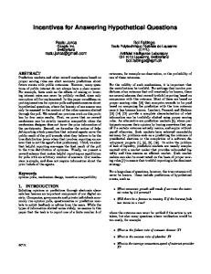
Since this problem is non-trivial to understand from the recurrences, we propose an additional illustration of a RNA chain folded according to the Zuker folding algorithm.
23
68
78
G A U A A C GA C A A G G G C G U C A C G C U CA U C AG C G U C G G C A C A U G C G U G 47 G A G C G A C C C A C C C U A G C U A G C U C C G A A U C C C G U G G G G G C G A C A G A C G C A U C G C G C G 11 G C G C A A A A A A A A C G C G G C G C A A A A A A 127 1
Types of structural features modeled by the Zuker folding algorithm include: dangling ends (1), internal loop (11), stack (23), multi-loop (47), bulge (68) and hairpin loop (78).
Figure 7: An example of an RNA folded into a secondary structure 8. Optimizations: notice that there are 3 matrices: W ,V (V BI is part of V ) that can be expressed using regular matrix, and F that is of different dimension than W and V and requires a special construction. Also notice that the k of BV and BW describe almost the same backtrack, but there is an additional cost c in BV . Alternative: Since the recurrence matrices described in [21] are of different dimensions (F matrix is O(n)), we might want to use another description [31] where all matrices are of the same dimension, such that we can have a more uniform description across DP problems: Let Q′(i,j) the minimum energy of folding of a subsequence i, j given that bases i and j form a base pair. Q(i,j) and QM(i,j) are the minimum energy of folding of the subsequence i, j assuming that this subsequence is inside a multi-loop and that it contains respectively at least one and two base pairs. A simplified model of the recursion relations can be written as: Eh(i, j) Es(i, j) + Q′i+1,j−1 if (i, j) is a basepair min min Ei(i, j, k, l) + Q′k,l Q′(i,j) = i
Qi,j
= min{QMi,j , Qi+1,j , Qi,j−1 , Q′i,j }
3
DYNAMIC PROGRAMMING PROBLEMS
DynaProg for Scala, p. 24
The corresponding energy functions are: • Eh(i, j) energy of hairpin loop closed by the pair i · j. • Ei(i, j, k, l) energy of interior loop formed by two base pairs i · j, k · l. • Es(i, j) energy of two stacked base pairs i · j and (i + 1) · (j − 1). This latter recurrence is more amenable to be converted into a grammar as the matrix are all of the same dimension. See the example in §6.1.2 for a detailed implementation of this problem.
3.3
Related problems
The aim of this section is to demonstrate that the problems previously described are very similar or encompass a significant part of the common dynamic programming problems18 . Serial problems
Shape
Smith-Waterman simple (§3.2.1) Smith-Waterman affine gap extension (§3.2.2) Needleman-Wunsch Checkerboard Longest common subsequence Longest common substring Levenshtein distance De Boor evaluating B-spline curves
rectangle rectangle rectangle rectangle rectangle triangle rectangle rectangle
Non-serial problems
Shape
Smith-Waterman arbitrary gap cost (§3.2.3) Convex polygon triangulation (§3.2.4) Matrix chain multiplication (§3.2.5) Nussinov (§3.2.6) Zuker folding (§3.2.7) CYK Cocke-Younger-Kasami Knapsack (pseudo-polynomial)
rectangle triangle triangle triangle triangle triangle rectangle
Matrices
Wavefront
1 3 1 1 1 1 1 1
– (can replace 2 matrices) – – – – – –
Matrices
Wavefront
1 1 1 1 3 #rules 1
– – – – – – –
Table 1: Classification of related problems 3.3.1
Other problems
• Dijkstra shortest path: can be expressed in DP and requires a E × V matrix. Informally: along E, forall V , reduce the distance. The problem is serial along the E dimension and non-serial along V , hence its complexity is O(|E| · |V 2 |) which is worse than both O(|V |2 ) (using a minimum priority queue) and O(|E| + |V | log |V |) (with Fibonacci heap). • Fibonacci numbers: this problem is serial 1D (in 1 dimension). F (n) could be implemented with ADP using a sequence of n placeholder elements, but this is inefficient. • Tower of Hanoi: 1D non-serial • Knuth’s word wrapping: 1D non-serial • Longest increasing subsequence: serial (binary search is more efficient). 18
There are hyperlinks on the problems name to their detailed description.
3
DYNAMIC PROGRAMMING PROBLEMS
DynaProg for Scala, p. 25
• Coin Change: 1D non-serial These algorithms also involve dynamic programming. However, we do not thoroughly evaluate their shape and number of matrices as a detailed description is not the focus of this project. • • • • • • • • • • • • 3.3.2
Floyd-Warshall Viterbi (hidden Markov models): T non-serial iterations over a vector Bellman-Ford (finding the shortest distance in a graph) Earley parser (a type of chart parser) Kadane maximum subarray 1D serial, look at Takaoka for 2D Recursive least squares Bitonic tour Shortest path, Shortest path in DAGs, All pair shortest paths, Independent sets in trees Subset Sum, Family Graph Optimal Binary Search Trees Independent set on a tree More dynamic programming problems from Wikipedia Conclusion
In the rest of the report, we use a different description of the problems that is based on ADP [15], which is more convenient but does not share much with the above description (even though ultimately the executed computations are very similar). Although not of immediate use, the description of the above problem and ad-hoc CUDA implementation of three of them (SmithWaterman with arbitrary gap cost, Matrix chain multiplication and Convex polygon triangulation) helped us to understand: 1. There is a difference between dynamic programming as seen in algorithmic schoolbooks and their concrete implementation, mainly because special care must be taken for correct indices and preventing off-by-one errors. 2. Problems can be classified in two categories: single track (input) and two-tracks (2 input sequences). Most of the interesting dynamic programming problems that could be parallelized fall in these two categories. 3. Sometimes matrices are initially padded with zeroes (or initial value), although this might be ignored at algorithm design, care must be taken for these special values and their inclusion in the matrix should be decided according to the complexity of the recurrence formula. 4. Incidentally, we proposed a cyclic variant of the convex polygon triangulation, which uses a parallelogram matrix (see §4.6). Unfortunately, this proved to be based on an erroneous recurrence relation analysis, and can only use a triangular matrix as described in §3.2.4. Although we have not found a real problem requiring a parallelogram matrix, we still present this version in §4.6 and §5.1. Such matrix layout could be adapted for cyclic problems that could be broken into a linear sequence anywhere (that is for all position in the circular structure, break the cycle at this position, and solve the dynamic programming problem on the resulting flattened sequence). For example, one could be interested in finding the longest subsequence verifying some property in a cycle, such that the subsequence score changes if it is rotated.
4
ARCHITECTURE DESIGN AND TECHNICAL DECISIONS
DynaProg for Scala, p. 26
4 Architecture design and technical decisions 4.1
User facing language requirements
The field of dynamic programming has been influenced in the recent years by a methodology known as Algebraic Dynamic Programming which uses a grammar and an algebra to separate between the parsing and the score computation: The Algebraic Dynamic Programming approach (ADP) introduces a conceptual splitting of a DP algorithm into a recognition and an evaluation phase. The evaluation phase is specified by an evaluation algebra, the recognition phase by a yield grammar. Each grammar can be combined with a variety of algebras to solve different but related problems, for which heretofore DP recurrences had to be developed independently. Grammar and algebra together describe a DP algorithm on a high level of abstraction, supporting the development of ideas and the comparison of algorithms. Given such formalization [15] of dynamic programming on sequences, it seems natural to borrow from it and extend it to other types of DP problems. In short, this framework allow the user to define a grammar using parsers, which are then run over an input string and produce intermediate results that are memoized into a table, when multiple solutions are possible, the user can define an aggregation function (h) to retain only some candidates for further combination. The benefits of the ADP framework is that it does not constrains the result of the evaluation to be a single value, but can extend parsers to backtracking parsers or pretty-printers. Additionally, we want to support the following features: 1. Input pair algebra: the original ADP framework [15] only support single input, we want to support pairs of inputs sequences similarly as [36] such that we can treat problem such as Smith Waterman or Needleman-Wunsch. As discussed in §??, handling more than two sequences introduces an Ω(n3 ) storage complexity that might limit more severely the size of problems that could be addressed. Since the problems seen in §3 use either one or two input sequences, we only need to support these two cases. 2. Windowing: this can be easily encoded by passing the windowing parameter that limits the computation, then it could be possible to collect either the best or k-best results. 3. Input restrictions: since CUDA (and FPGA) cannot process arbitrary Scala objects, we need to restrict the language to primary types (int, float, ... and structures of them). However, we want to preserve the expressivity available in Scala and impose restrictions on the data types processed by CUDA. A typical restriction we want to make is that data elements are of fixed size, to avoid memory management issues and thread divergence19 . 4. Single-result on devices: The general ADP framework supports multiple solutions for intermediate results. Such functionality is easily supported in Scala; however, memory management hampers the performance of the GPU implementation (see §2.5). To overcome this issue, the user could manually manage the memory, but this would defeat most of the benefits of automatic code generation. Hence the trade-off solution we propose is to restrict ADP to only one optimal result on CUDA, while offering the possibility to obtain co-optimal (or even all possible solutions) with Scala. 5. Automatic backtracking: To produce efficient code, we imposed a fixed size on the output generated by the parsers on devices. However, on the other hand, the backtracking information (of varying size) is of primary interest for the DSL user, hence we would like 19
Occurs when a single thread needs more processing than its peers, thereby delaying the whole computation.
4
ARCHITECTURE DESIGN AND TECHNICAL DECISIONS
DynaProg for Scala, p. 27
to to automate the backtracking to fulfill goals of usefulness, efficiency and ease-of-use in device-specific implementation: • Leaving the backtrack implementation to the user would force him to memoize the backtracking information together with the results (backtrack would grow towards final result and duplicate unnecessarily information), hence requiring both O(n3 ) space and memory management features on devices. • Enforcing automatic backtracking presents the advantage to ensure constant size for intermediate results, hence ensuring an O(n2 ) storage requirement. Collecting the backtracking list can be easily done in O(n) and then reversed depending on whether we prefer bottom-up or top-down construction (the backtrack is usually a lattice of nodes that constitute a tree whose leaves are input elements). 6. Yield analysis: in vanilla ADP, the user has to define for each concatenation the minimal and maximal length of the subsequence on each side. Although non-emptiness information is necessary to avoid infinite recursions in the parsers, forcing an explicit definition can become cumbersome for the DSL user. Similarly as in [17], we want to provide an automatic computation of concatenation boundaries, while at the same time leaving the possibility to manually specify it for maximum flexibility. The support of these features has the following implications: • Dependency analysis: Since we target GPUs (and FPGAs) which are massively parallel architecture, a top-down execution using hash tables is impractical (fallback computation if element is not present is hard to parallelize), hence we need to construct the result tree bottom-up, therefore ensure that the (partial) evaluation order between rules is respected. • Normalization: in order to automate the backtracking, we need the grammar rules to present a certain shape so that we can define uniquely the backtracking information (in particular we want to distinguish between alternatives). Also we need to maintain coherence between the Scala and the CUDA version so that they can inter-operate: we would like to reuse the backtracking information (from CUDA) to do actual processing in Scala (pretty-printing or actual computation as described in §1). • Optimizations: Since ADP exposes a grammar, we might have the opportunity to do optimizations at the grammar level (see §4.1.1). Also since the grammar might define useless rules, we might want to eliminate them: dead rule elimination is very similar to traditional dead code elimination (it reduces the size of generated code) but also reduces the memory consumption (as storage matrix does not need to be reserved) and even speeds up the computation, (since all grammar rules for a particular element are computed at the same time in CUDA implementation, see 4.2.1). 4.1.1
Grammar optimization
Since ADP exposes a grammar, we might be able to break complex grammar rules into simpler ones (optimally binary production). For example, consider the following rule (in BNF): { ′ A := B X A := B C D =⇒ X := C D If B, C and D are of varying length, evaluating the rule A for a single subproblem is O(n2 ) (assuming B,C,D are stored in matrices hence O(1)). Adding a tabulation X reduces the evaluation complexity because for each subproblem we will consider either rule A′ or X, each of evaluation complexity O(n); hence we would have reduced the grammar evaluation complexity.
4
ARCHITECTURE DESIGN AND TECHNICAL DECISIONS
DynaProg for Scala, p. 28
Since grammar candidates are then evaluated with an algebra, we need to devise an equivalent transformation of the algebra. Unfortunately this analysis is very involved: we need to solve the following problem (to respect Bellman’s optimality principle[3]): Given f , find a pair of functions (f1 , f2 ) or (f3 , f4 ) such that20 ∧ ∨
min
[ f (i, k1 , k2 , j)] = f1 (i, f2[(i, k1 , k2 ), k2 ,[j) ] ] f (i, k1 , k2 , j) = min f1 (i, min (f2 (i, k1 , k2 ) , k2 , j)
min
[ f (i, k1 , k2 , j)] = f3 (i, k1[, f4 (k1 , k2 , j), j) [ ] ] ∧ f (i, k1 , k2 , j) = min f3 (i, k1 , min (f4 (k1 , k2 , j) , j)
i
i
i
i
i
k1
Since this requires complex mathematical analysis that is out of the scope of the project, and since we have not found relevant literature on that particular subject, we leave this optimization to the responsibility of the user by assuming that the provided grammar is already optimal. Note that this optimization needs to use informations from both the grammar (the rule to split) and the algebra (f ), which restricting its application to either single algebra or algebra that could share the same optimization, because modifying the grammar will change the associated backtrack information (thereby breaking its compatibility for usage with other algebras).
4.2
Recurrences analysis
In this section we use the following notation: let A be a tabulation parser, we refer by A(i,j) to the element i, j of the underlying matrix (in order to keep a lightweight notation). 4.2.1
Dead rules elimination
Dead rules21 elimination analysis is straightforward: starting from the grammar’s axiom, recursively collect all tabulations involved in the computation in R (set of rules that are reachable from the axiom). The dead rules D = S \ R (where S is the set of all tabulations) can safely be removed from the grammar rules. Although seemingly useless for the Scala implementation, this step is necessary to maintain coherency between Scala and CUDA rules numbering (that happen in a later stage on the valid rules). In CUDA, this analysis not only provides dead code elimination, but it also prevents useless computation execution, since all rules are computed sequentially for a particular subsequence before the next subsequence is processed. 4.2.2
Yield analysis
Since the original ADP introduces many concatenation combinators22 to differentiate empty/nonempty, and floating/fixed-length concatenations, it is quite involved for the programmer to make sure that the concatenation operators exactly match the size of each pair of subsequence involved. Additionally the priority of operators varies in Scala, depending the operator’s first character whereas it is possible to specify arbitrary priorities in Haskell. To overcome these issues, we propose to automate the computation of the minimum/maximum length of (subsequences) parsers. 20
The first and third equations denote breaking in two distinct functions, the second and fourth represent Bellman’s optimality principle preservation. 21 Rule denotes a tabulation belonging to the grammar; both terms refer to the same concept, with the subtle difference that rule emphasizes its grammar membership. 22 ADP’s original combinators are: ∼∼, ∼∼ ∗, ∗ ∼∼, ∗ ∼ ∗, − ∼∼, ∼∼ −, + ∼∼, ∼∼ +, + ∼ +.
4
ARCHITECTURE DESIGN AND TECHNICAL DECISIONS
DynaProg for Scala, p. 29
Parsers are made of terminals, concatenations, operations (aggregate, map, filter) and tabulations; minimum/maximum yield of terminals is set, hence it only remains to assign appropriate yield sizes to tabulations; other operations simply propagate that information. It is possible to obtain the yield size of tabulations using the following algorithm (assuming recursive parsers contain at least one tabulation that is part of the loop), similar to [18]: 1. Set the yield minimum size of all tabulations to a large number M0 (such that all tabulation would reasonably have a minimum yield size smaller than M0 ) 2. Repeat k times (k is the number of rules of the grammar): for each rule, compute its minimum yield size and update its value (without recursion at tabulations). This would lead to a correct minimum yield size because the terminals provide a minimum size and this might need at most k iteration to propagate across all rules. 3. Set the maximal yield of all the rules to the minimal value. For each rule, compute recursively up to depth k (where the depth is computed as the number of tabulation traversed) the maximum yield size. If the depth reaches the maximum k, there is a loop between tabulations, hence return infinity. The last part of this algorithm has worst case exponential complexity, but if we consider depthfirst search and return as soon as we reach infinity, we might reduce its complexity to O(k 2 ). Obtaining the yield size of tabulations provides the following benefits: • Minimum size: prevents self-reference parsers (on the same subsequence) and avoids considering subsequences which yield empty results (hence slightly reducing time complexity). • Maximum size: allows to reduce the size of the result and backtrack matrix to O(m · n) instead of O(n2 ) (where m is the maximum yield size), possibly providing substantial space savings. As the rules with bounded maximum yield are very rare, we did not implement this optimization, although we might consider it for future work. 4.2.3
Dependency analysis
Let us introduce the concept of dependency (similar to →chain in [18]): a dependency between tabulations A, B denoted A → B exists if B(i,j) = f (A(i,j) ), that is if the result of B depends of the result on the same subproblem computed in A. A grammar is unsolvable if there exists a dependency loop between parsers (A → ... → A). Such case only happen when there is no concatenation or a concatenation with an empty word. Being able to track the dependencies of tabulations and infer a computation order between them has two benefits: • Although seemingly unnecessary in a top-down approach (Scala), this analysis detects dependency loops which would result in infinite call loops (stack overflow) at execution. • Ordering tabulations is critical in a bottom-up approach (CUDA) to make sure that all dependencies are valid before an element computation is triggered.
4
ARCHITECTURE DESIGN AND TECHNICAL DECISIONS
4.3
DynaProg for Scala, p. 30
Backtracking
In order to produce an efficient transformation from an ADP-like problem description to plain C recurrences, we need to construct bottom-up recurrences from top-down parser rules. To do that, we slightly need to modify the ADP parsers in order to separate the backtracking and the scoring, because we want to obtain an efficient algorithm: backtrack writes are in O(n2 ) whereas score reads are proportional to the algorithmic complexity (O(n3 ) or more for non-serial). To deal with this problem, we are facing two options: • Explicit backtracking: requires clear syntactical separation between the score and the backtrack which is not implemented in ADP, unless we consider the whole backtrack being part of the scoring (which has a big performance impact and non-constant memory requirement issues that make such GPU implementation hard and not desirable). Additionally, since the backtracking data is user-defined, there is no way to generate the backtracking algorithm automatically, hence the user also needs to provide it. • Implicit backtracking: implies that every rule needs to be normalized, and transformed such that given a rule identifier and a set of indices (subproblems breaking), it is possible to retrieve the sub-solutions combination that contribute to the problem solution. To do that we need to apply the following transformations 1. Normalize rules and identify them uniquely by exploding alternatives: each rule is decomposed into the union of multiple sub-rules uniquely identified by an index, where sub-rules do not contain alternatives (Or parsers). Let s a subrule and rs its identifier, we also establish a mapping T from identifier to subrule: (rs → s) ∈ T . 2. Let cc(rs ) be the number of concatenation contained in the sub-rule rs . The data element corresponding to a rule is a pair (score, backtrack) and is named after the tabulation. – The score part consists of a user-defined type (a composite of primitive types, case classes and tuples) – The backtrack part is a tuple (rs , (k1 , k2 , . . . , km )) where m is the maximal number of [concatenations occurring in the enclosing rule of rs ; more formally ] m = maxz cc(rz )|rz ∈ rule(rs ) , and let ms = cc(rs ) ≤ m. 3. During the matrix computation of cell (i, j), if the sub-rule rs applies, the backtrack will be set as (rs , (k1 , k2 , . . . , kms )); with i ≤ k1 ≤ k2 ≤ . . . kms ≤ j. Note that if the backtrack occupies a fixed-length memory, the backtrack will contain exactly m indices, hence ki | ms < i ≤ m will be unspecified. 4. During backtracking, when reading the cell (i, j) with backtrack (rs , (k1 , k2 , . . . , km )), given rs , we recover s = T (rs ), the sub-rule that applies. Hence we can determine ms , which allows us to enqueue the subsequences (i, k1 ), (k1 , k2 ), ..., (kms , j) for recursive backtracking. If s refers to a terminal, we stop the backtracking. 5. The backtracking can be returned to the user as a mapping table T and a list of triplets ((i, j), rs , (k1 , k2 , . . . , kms )) where (i, j) denotes the subsequence on which the sub-rule T (rs ) has to be applied with concatenation indices (k1 , k2 , . . . , kms ). In short, we break parsers into normalized rules, the backtracking information is the subword, the sub-rule id (which rule to unfold) and a list of indices (how to unfold it). In order to reduce the storage required by the backtracking indices, we can avoid storing fixed indices (where at least one of the two subsequences involved in a concatenation has a fixed size) and leverage the knowledge contained in s to reconstruct the appropriate backtrack.
4
ARCHITECTURE DESIGN AND TECHNICAL DECISIONS
DynaProg for Scala, p. 31
Assuming that the backtracking information is meant to guide further processing, we provide this information into a list constructed bottom-up: it can be simply processed in-order, applying for each rule the underlying transformation, while intermediate results are stored (in a hash map) until they are processed by another rule. Since there is only one consumer for each intermediate result, every read value can be immediately discarded, thereby reducing the memory consumption. Ultimately, only the problem solution will be stored (in the hash map). 4.3.1
Backtracking with multiple backtrack elements
The backtracking technique described above work fine when there is a single element stored per matrix cell (which is usually the case with min/max problems). However, in the generalization introduced by ADP, it is possible that a matrix cell stores multiple results. In such case, we need to select a correct intermediate result to avoid backtracking inconsistencies. Additionally, we need to keep track of the multiplicities of the solutions, that is if we want to obtain the k best solutions, we need to make sure that we return k different traces. To do that, we maintain a multiplicity counter in each backtrack path: • While there is an unique solution for all possible incoming paths, we continue in this direction with the same multiplicity (we have no choice). • When there is r different solutions available, and the path multiplicity at this point is k we have the following cases: 1. If k ≥ r: we explore all paths with multiplicity k − r + 1. This is because each branch may produce only one solution and we don’t know ahead of time which path will provide multiple solutions. Finally, we retain only the k best solutions. 2. If k < r (there is more paths than needed): we explore the k first paths with multiplicity 1 and safely ignore the other (as we only need k distinct results). Now remains the problem of generating all possible results and check whether they are valid candidates. To do that we simply re-apply the parsers while maintaining the source elements of all production and then retain only those with desired score and backtrack. Since we know the backtrack for one element, we can do the following optimization at backtrack parser computation: 1. Defuse alternatives: since we know exactly (by the subrule id rs , maintained in the backtrack) which alternative has been taken to obtain the result, we can skip undesired branches of or parsers. 2. Feed concatenation indices: since the backtrack stores the concatenation indices, we can reuse in the concatenation parsers. This removes the O(f (n)) factor in the backtrack complexity (as concatenation backtrack parsers «know» where to split). 3. Skip filters: since filters are applied before their inner solution is computed, they are only position-dependent. Hence if a backtrack involves a filter, since its position is set by the backtrack, the filter must have been passed at matrix construction time. 4.3.2
Backtracking complexity
Since the ADP parsers can store multiple results, we are interested in measuring the overhead of k-best backtracking (compared to single-element backtracking). For single-element backtrack, we only need to «revert» the parser to find involved subsequences, which is linear in the parser size (because the backtracking identifies uniquely the alternative and concatenations indices).
4
ARCHITECTURE DESIGN AND TECHNICAL DECISIONS
DynaProg for Scala, p. 32
At every backtrack step, either: • The sequence is removed at one element, which leads to maximal backtrack length of n. • The sequence is split in k subsequences, with recurrence f (n) = k · f (n/k) + 1 by solving this recurrence we see that there can be at most n final nodes and n intermediate nodes (when k = 2). Hence the backtrack length is at most 2n. Let one parser reversal complexity be O(p), single backtrack has O(2n · p) complexity. For the k-elements backtrack, since we regenerate all possible solutions, that is O(k c+1 ) candidates (with c the maximal number of concatenation in the parser), the overall complexity is O(2n · k c+1 · p). Hence there is a k c+1 factor to pay if we want to backtrack the k best solutions23 . Another special case we might be interested in is to obtain all co-optimal solutions (all the solutions that have an optimal score). We can notice that in the parser reversal, no sub-solution is discarded, because either it is not co-optimal (and would have been discarded at an earlier stage) or it is co-optimal, hence contributes to create a co-optimal result. It follows that the complexity of co-optimal solutions backtrack is proportional to the number of solutions. 4.3.3
Backtrack utilization
Since the dynamic programming may help solving a larger problem24 , we need to be able to apply the result of the dynamic programming computation in a different domain. The easiest way to do that, is to reuse the same input and grammar, but use a different algebra with a different output domain, and only compute the result of the trace obtained from the DP backtrack. This step is pretty straightforward: since ADP parsers emphasize on the split between signature and grammar and decouples them, we only need to modify the algebra to operate on another domain, and reuse the same grammar. The key point here is to notice that a backtrack trace of a parser can be reused by another, providing that they share the same grammar. For instance, to compute optimally a matrix chain multiplication, we solve the DP problem in a domain where matrices are represented by their dimensions, we obtain an optimal trace and feed it to another parser operating on «concrete matrices» domain that will do the actual matrix multiplication (instead of the cost estimation).
23
Note that the same kc+1 factor lies in the forward matrix computation complexity. For instance in matrix chain multiplication, we only care about matrix dimensions for dynamic programming, however, we ultimately want to multiply the real matrices and obtain a result. 24
4
ARCHITECTURE DESIGN AND TECHNICAL DECISIONS
4.4
DynaProg for Scala, p. 33
CUDA storage: from list to optional value
Since lists are natively supported, it is natural to gather parsers results into lists in Scala implementation. However, when it comes to efficient CUDA implementation, lists must be avoided because memory allocation (and management) is not very efficient [38]. A workaround might be to use fixed-length lists but we assume here that the programmer is most often interested in a single optimal solution (this also alleviates the complexity of constructing multiple distinct backtrack traces). Even if this restriction simplifies the design, issues might arise for how to represent and deal with empty lists and how to minimize the amount of used memory: • Minimizing memory consumption: Under the restriction that we only store the best result, we first need to transform aggregation such that they return at most one element. Useful aggregator belonging to this class are quite limited: minimum/maximum (optionally with respect to an object’s property), count and sum25 , hence it is possible to provide the user with a tailored implementation. To benefit from this fixed memory aggregation, we need to do some structural transformation of inner parsers. In general, a tabulation T is the root of its evaluation tree, with leaves being either other tabulations or terminals, note that any of the 5 intermediate element can appear multiple times (or not being present) and in any order: T < Aggregate < Or < Filter < Map < Concat < (Tabulation | Terminal) For obvious performance reasons, we want to maintain aggregations wherever they are present. However, we can partially normalize the rest of the evaluation tree: – We must ensure that all parsers potentially generating multiple possibilities are aggregated. To do that, we simply wrap the original parser in an h-aggregation (where h is the default aggregation function that must be specified by the user) – Since the aggregation now operates on a single element, we want to push it as close to the leaves as possible, as long as we do not change operational domain26 . – Filters can be hoisted within the same concatenation / alternative – Alternatives must be hoisted outside of maps and concatenations, the reason being that we need to avoid maintaining lists of candidates (that will be later aggregated). We summarize the required transformations in the following table: Outer ⧹ inner Aggregate Or Map Filter Concat
Aggregate merge? — — — —
Or swapR simplify? swapR — swapR
Map — — fuse — —
Filter swapP swapP ? swapP merge? —
Concat — — — — —
R = required, P = performance optimization, ? = if possible
Table 2: Parsers normalization towards CUDA code generation Note that there can be no swap with Map and Concat internal parsers due to domain change. Fusing is done by the C compiler (declaring mapping functions inline). 25 26
Notice that all these operations can be implemented with a folding operation on a single variable. We cannot push an aggregation through a mapping or a concatenation operation.
4
ARCHITECTURE DESIGN AND TECHNICAL DECISIONS
DynaProg for Scala, p. 34
• Handling nested aggregations: since a tabulation might contain nested aggregations, they must be preserved in order not to increase its time complexity. To do that, each internal aggregation has to define its own intermediate score and backtrack variables, whereas outermost aggregation can directly write in the cell of the cost/backtrack matrix. • Failure handling: a parser can either be successful and return results or fail and return no result (encoded as an empty list); failure can happen in terminals, (input) tabulations and filters. These 3 cases can be reduced to one by wrapping terminals and tabulations into a filter that checks validity conditions. It remains to discuss failure encoding strategies: – Special «empty» value: The benefit of such encoding is a reduced number of memory accesses; indeed since we anyway need to access the value to make computations, we do not generate additional memory accesses to check the validity of the value. The drawback of such approach is that it becomes necessary to specify a special empty value that cannot be used, except to denote the absence of result. Since types can be arbitrary at every step of the parser, it becomes cumbersome to ask the DSL user to provide a special value for every intermediate result. – Backtrack encoding: Reusing the backtrack to encode the validity of a result is a more general approach, and allow greater flexibility for the user. Indeed, since we maintain sub-rules identifiers in the backtrack, it suffice to use a special identifier to denote that related value is invalid. This approach also work with nested aggregations by storing intermediate sub-rule identifiers that would only grant the validity of the related value. Since backtrack encoding comes at the price of an additional memory access to test the validity (memory accesses usually accounts for most of the time on CUDA devices), it is also relevant to allow the user to completely disable this test to speed-up computations.
4.5
Memory constraints
We denote by device the computational device on which the processing of the DP matrix (or of a computational block) is done and MD its memory. This can be the GPU or the FPGA internal memory. Usually the main memory is larger than device memory and can ultimately be extended by either disk or network storage. Without loss of generality, let the underlying dynamic programming matrices be of dimension m × n. We propose to evaluate the device memory requirements to solve the above problem classes. We need first to define additional problem properties related to implementation: • Number of matrices: multiple matrices can be encoded as 1 matrix with multiple values per cell. Hence the implementation differentiates only between cost and backtrack matrices with respective element sizes SC and SB . • Delay of dependencies: In case the problem does not fit into memory, partial matrix content needs to be transferred across sub-problems. Such data amount is usually proportional to the delay of dependencies. If this delay is small, it might be worth to duplicate matrix data in the wavefront, otherwise it might be more efficient to allow access to the previous computational blocks of the matrix. • Wavefront size: Finally aggregations that are made along the dimensions of the matrix do not need to be written at every cell but can be propagated and aggregated along with computation (ex: maximum along one row or column). Hence such information can be maintained in a single place (in the wavefront) and progress together with the computation.
4
ARCHITECTURE DESIGN AND TECHNICAL DECISIONS
DynaProg for Scala, p. 35
We denote by SW the size of wavefront elements. • Input size: the size of an input symbol (from input alphabet) is denoted by SI . 4.5.1
Small problems (in-memory)
Problem that can fit in memory can be solved in a single pass on the device. Such problem must satisfy the equation: (SI + SW ) · (m + n) + (SC + SB ) · (m · n) ≤ MD For instance, assuming that m = n, MD = 1024Mb, that backtrack is 2b (<16384, 3 directions) and that the cost can be represented on 4 b (int or float), that input is 1b (char) and that there is no wavefront, we can treat problems of size n such that 2n + 5n2 ≤ 230 =⇒ n ≤ 14650. We might also possibly need to take into account extra padding memory used for coalesced accesses. But it is reasonable to estimate that problems up to 14K fit in memory. 4.5.2
Large problems
To handle large problems, we need to split the (m × n) matrix into blocks of size BH × BW . For simplification in our estimations, we assume a square matrix (m = n) made of square blocks with b blocks per row/column (BH = BW = n/b). 4.5.3
Non-serial problems
Non-serial problems need to potentially access all elements that have been previously computed. We restrict ourselves to the following dependencies27 : • Non-serial dependencies along row and column • Serial dependencies along diagonal, with delay smaller or equal to one block size Such restriction implies that all the block of the line and the row, and one additional block to cover diagonal dependencies must be held in memory (independently of the matrix shape). Hence we have the following memory restriction: n n2 n2 2 (SI + SW ) + 2 · SC + 2 SB ≤ MD b b b We also need to take into account the transfer between main memory (or disk) and device memory. Dependency blocks only need to be read, computed blocks need to be written back. Ignoring the backtrack and focusing only on the cost blocks, the transfers (in blocks) are: b−1 ∑ b2 + (b − 1)2 + i · b = 12 b3 + 32 b2 − 2b + 1 i=0 ) b ( ∑ 1 + 2 · (i − 1) · (b + 1 − i) = 13 b3 + 12 b2 + 61 b i=1 ) b ( ∑ 1 + 2 · (i − 1) · b = b3
(Rectangle) (Triangle) (Parallelogram)
i=1
Putting these two formula together, and using most of the device memory available, we obtain the following results with SC = 4, SB 28 = 4, SI = 1, SW = 0 and MD = 230 : 27 28
As we have not encountered a problem with non-serial dependencies along the diagonal. To deal with larger matrices, backtrack data need to be extended.
4
ARCHITECTURE DESIGN AND TECHNICAL DECISIONS
DynaProg for Scala, p. 36
9000 Rectangle Triangle Parallelogram
8000
Data transferred (GB)
7000 6000 5000 4000 3000 2000 1000 0
0
2
4
6
8 Input size
10
12
14 4
x 10
Figure 8: Transfer overhead for non-serial problems larger than device memory Given an experimental bandwidth of 5.3743 Gb/s between CPU and GPU, processing matrices one order of magnitude larger (128K) would result in respectively 13(R) , 8.5(T) and 25.4(P) minutes of transfer delay. Extrapolating the preliminary results of small problems, a computation on input of size 128K would require respectively 7 days 13h(R) , 2 days 22h and 6 days 10h(P) , assuming there is no other scalability issues, hence transfer would account respectively for 0.1%(R) , 0.2%(T) and 0.3%(P) of the running time. Although this overhead seems appealing compared to the computation time, the total running time blows up (because of the O(n3 ) complexity) and make the processing of such large problem less relevant. Given that real problems (like RNA folding) operate on sequences length in the hundreds [31], it would not be of much relevance to implement a version for larger cases, although perfectly feasible. 4.5.4
Serial problems
The serial problems have the interesting property to access a fixed number of previous elements. These elements can be stored either explicitly in a scoring matrix, or implicitly into the wavefront (as moving aggregations). Since the dependencies are fixed, the computation direction gains an additional degree of freedom: the matrix can be solved in diagonal (as non-serial problems), line-wise or column-wise. This allows to store the whole necessary state to make progress into a limited number of lines (or columns), and sweep vertically (resp. horizontally) along the matrix. Since serial problems are of complexity O(n2 ) (due to the matrix dimension and the finite number of dependencies), it is possible to tackle much larger problem than non-serial given the same running time. Hence, it seems natural to let serial problems grow larger than the memory. Mixing the dependency property and size requirements, we can split the matrix into submatrices, store special lines (and/or columns) into memory (or hard disk), and repeat computations to solve the backtrack (similarly as in [34],[12], but this implementation use problemspecific knowledge that might not generalize).
4
ARCHITECTURE DESIGN AND TECHNICAL DECISIONS
DynaProg for Scala, p. 37
To store intermediate lines and columns, we are facing two different strategies to explore: • Fixed subproblem size: we decompose the algorithm as follows 1. Define a grid of «major column and rows», where each cell’s data (input, output, cost and backtrack matrices) fits into the device memory. 2. Compute the values of the grid’s major columns and rows in one pass. 3. Second (on-demand) computation to process backtracking inside relevant cells. Let b the number of cells that we have on each row/column, the total computation running time would be (b2 + 2b) · tb where tb is the time to compute one cell’s matrix. This division has the advantage of providing the minimal computation time at the expense of external storage proportional to O(n) (if we store only lines or columns) or O(n2 ) (if we store both). • Myers and Miller’s algorithm: [26] (divide and conquer) This algorithm break the DP problem into 2 (or 4) subproblems such that once the middle line/column is computed, the problem can be solved for one submatrix while backtracking occurs in up to 3 other submatrices. This breaking is applied recursively until the submatrix data fits into memory. The storage requirements are 4 · O(n) (we store along both dimension 1 + 12 + 14 + ... lines/columns). The algorithm proceeds as follows: first it solves the problem of obtaining the first backtracking element, then it breaks the matrix in 4 submatrices, and refine it until backtrack is tractable. Since there is at most log n/b refinements and since every part of the matrix may be involved in backtrack, running time is O(n2 log2 n). • Hybrid approach: [13] a hybrid approach might be created to take advantage of additional available memory, however, the running time decreases logarithmically to the space used, this means that using 4× more storage space would only result in a 2× speedup (measuring only the computation time). Hence a hybrid approach would be to decide a k such that at each step, we partition the desired sub-matrix into a intermediate grid of k rows/columns. The space usage would be in 2k logk (n/b) and the running time complexity would be O(n2 · logk n). Then the user would be able to fix a storage space S ≥ 4 log2 (n/b) and obtain the corresponding k for a given n. Finally, although such problem is interesting because targeted platforms could include FPGA, where efficient implementations exist [42], several reasons made us considering this class of problem as a future work: • The most prominent problem in this category is Smith-Waterman, for which efficient implementation already exists[34],[12]. Additionally, the authors are planning to write extensions to support some variants of this problem like Needleman-Wunsch. • The implementation sensibly differs from the class of small problems, as the solving strategy is completely different from non-serial small problems, thereby requiring larger development time that would be out of the scope of this project. • Finally, such an implementation would be only valuable for problems that are larger than the memory device, whereas smaller problems could perfectly use the existing implementation.
4
ARCHITECTURE DESIGN AND TECHNICAL DECISIONS
4.6
DynaProg for Scala, p. 38
Memory layout
A major bottleneck on massively parallel architecture with shared memory (like CUDA) is the global memory access. To address it, according to the manufacturer documentation [27], it would be best if all threads access contiguous memory at the same time (coalesced memory access). This is justified by the memory hardware architecture, where additional latency (precharge rows and columns of the memory chip) is mandatory to access data at very different positions. Since all thread share the same global memory (and most of the time the same scheduler), accessing non-contiguous memory cumulates latencies before progress can be made.
Triangle
Rectangle
Parallelogram
Figure 9: Matrix shapes, the arrow indicates the computation progress direction Because dependencies are along line, column or intermediate elements (§3.2), parallel progress can be made along the diagonal of the matrices, a naive row/column addressing strategy would result in no coalesced accesses. Hence we address them by diagonal. Let MW the width of the matrix and MH its height. Coalesced addressing is most easy in the parallelogram matrix, as we could pretend that the parallelogram is simply a tilted rectangle (with diagonal elements being contiguous in memory) as follows: (i, j) → i + (j − i) ∗ MH Noticing that the triangle matrix shape is just half the parallelogram, we could use the same addressing scheme, but we would use twice more memory than necessary. Hence we need a tailored formula: the size of the triangle embedded in a square of side k (incl. diagonal) is k·(k+1) ; knowing that fact, the index of the element (i, j) of the triangle (starting with the main 2 diagonal when i = j), we obtain the following formula (with MH = MW = n): (n · (n + 1) M = total △ 2 d = n + 1 + i − j diagonal of (i, j) (i, j) → M − T + i with (d · (d + 1) T = △ of current diagonal 2 Finally, for the rectangular matrix, since the parallelogram indexing looks efficient, we want to reuse the same idea. However, embedding the rectangle within a parallelogram would have a very large overhead ((MH )2 , by adding a triangle on each side of the rectangle). The solution consists of breaking the rectangle into multiple horizontal stripes of fixed height BH , thereby dramatically reducing the size of the additional triangles. Finally, the stripes can be stitched together to form a single parallelogram continuing along the next stripe. Noticing that beyond a certain number of lines, coalescing access does not improve latency as memory is anyway not stored contiguously, we can make BH constant .
4
ARCHITECTURE DESIGN AND TECHNICAL DECISIONS
DynaProg for Scala, p. 39
Figure 10: Parallelogram memory representation of a rectangular matrix It follows that the total memory required to store the matrix is: ⌉ ⌈ MH · BH + (BH )2 MW · BH and the mapping of indices is given by: ⌊
i (i, j) → (BH · (j + m) + m + BH diagonal
⌋ · MW · BH ) with m = i stripe size
mod BH
stripe
4.7
LMS integration
At first glance, LMS seems the ideal candidate to transform Scala code into its C-like equivalent. However, the concern in this project is that the GPU code sensibly differs from the original CPU code because the two implementations serve different purposes: CPU version (Scala) is more general whereas the GPU version trades some functionalities for performance and suffer additional restrictions, in particular for memory management and alignment. We want to discuss how LMS could best be used in our project: LMS only supports a subset of Scala. Embedding both algebras and grammars into the LMS framework would reduce the expressivity of algebras. Taking the example of matrix multiplication, the user would like to not only solve the dynamic problem on GPU, but also leverage the graphic card, the disk or the network to compute the matrices products. Since these resources are outside for the LMS world, the user needs to write an ad-hoc DSL for every particular function. In order to avoid this constraint, we need to decouple the grammar and algebra generation. For the generation of algebra functions, since CUDA types are restricted, they are representable in LMS. Hence we can leverage LMS for CUDA-compatible algebras whereas regular Scala can be used for complex algebras being executed on CPU exclusively. It remains to generate the C code corresponding to the grammar; we argue in favor of a specialized conversion rather than generation through LMS for the following reasons: • We have only 6 parser classes to convert (tabulations, terminals, aggregations, filters, alternatives, concatenations), the rest of the user program is part of the algebra. These parsers are combined with very little modifications to create the grammar. • The behavior of the CUDA parsers sensibly differs from that available in Scala (§4.4). This would imply writing optimization phases in LMS to convert them appropriately. • LMS operations on collections (lists, hash maps, arrays, ...) do not require special scheduling as all elements are treated independently; nevertheless dynamic programming introduces dependencies between elements, thus requiring particular scheduling interleaved with the computation. Enriching LMS with primitives to solve these constraints might be very
4
ARCHITECTURE DESIGN AND TECHNICAL DECISIONS
DynaProg for Scala, p. 40
complex if we want to generalize. However, we could leverage the knowledge that the pattern belongs to dynamic programming, hereby reducing the complexity of the work and possibly being more efficient. Additionally, a specific memory pattern is required to increase efficiency (§4.6), we also need to reuse this knowledge to LMS, so that it can generate optimal code, so we might end up writing a specialized code generator. • Finally, LMS is a rather complicated framework, with sparse documentation. Although many features are available (support for tuples, objects, matrices, ...), it is not easy to figure out where to find them (because they may reside on different branches or are not tested), hence the time taken to improve the framework to suit our needs far outweighs the time to build a tailored solution, which is the choice we are somehow forced to take, given the time constraints of this project. Since we need to operate a lot of transformation, inside LMS or in specialized generation, the choice of specialized code generation was guided by the engineering principle of steering away from unnecessary complexity29 , hence reducing the number of potential sources of errors. During our experiments with LMS, we also investigated in the Scala 2.10 macros30 [5], which represent a possible alternative to LMS for generating very simple functions for a costing algebra.
4.8
Compilation stack
Since the generated code sensibly differs from the Scala version, due to the reasons previously discussed, we cannot reuse LMS, although we borrow some of its ideas. Having the full control on the compilation stack also provides us the following benefits: • Since CUDA target and runtime compilation/execution is not supported in LMS, but in Delite [8]: an additional framework that runs on top of LMS. Although conceptually very similar, implementing our own stack reduces the number of dependencies, hence possible sources of misconfiguration errors for the final user of our framework. Additionally, since we do not share much of the functionality of Delite, an ad-hoc stack helps keeping the project featherweight. • LMS can generate code for monadic functions that operate on arrays. However dynamic programming problems might require multiple inputs (for multi-track grammars) and special scheduling (to respect dependencies in the matrix), hence we need to issue specific C/CUDA code to handle problems correctly. • LMS works on array of primitive types, possibly array of structures broken into array of simple types. Since in DP problems, composite types represent a single logical element, and since we want to benefit from coalesced accesses (and possibly storing structures into efficient on-chip shared memory), we do not want to break structures. Also we want to offer support for tuples, which are a convenient way to write data containers (also we want to support case classes and composites types). • Some information is only known at run-time (for instance input and matrix dimensions), hence we want to benefit from this knowledge as it helps computing the matrix indices more efficiently. Since such information could possibly be reused, we want to make the process as transparent as possible for the DSL user. 29
KISS engineering principle: http://en.wikipedia.org/wiki/KISS_principle (Macros operate directly on the internal representation of the Scala compiler, after the type analysis and and before the code generation phase. 30
4
ARCHITECTURE DESIGN AND TECHNICAL DECISIONS
DynaProg for Scala, p. 41
Finally, we reap most of the LMS benefits in the generation of user-defined functions, as they are completely independent of the rest of the generated program thus could be generated without additional processing. Although our compilation stack might look quite similar to that of Delite, we do not share any component but LMS for the user functions generation. The compilation and execution process works as follows: • Compilation: LMS generates the C code corresponding to the user-defined function and embeds them into the program bytecode (note that we present them separately for clarity). • Runtime, for each parser (grammar+algebra): recurrences analysis is done in order to generate code (with placeholders for constants) • Runtime, at every parse function call: the input size is known, hence replaced into the generic problem code, which is then processed by CUDA, C++ and Scala compilers. Then the JNI library resulting of the compilation is loaded and its corresponding Scala wrapper is invoked on the data to be processed.
DSL libraries
User program
Scala compiler
LMS
JVM bytecode
C functions compilation run-time
C/CUDA/JNI code recurrences analysis code generation
constants evaluation compilation
Scala parsers
JNI / host C
input size
CUDA kernels
Scala wrapper Input data Output data
Figure 11: Compilation and execution scheme of a parser
5
IMPLEMENTATION
DynaProg for Scala, p. 42
5 Implementation 5.1
CUDA baseline
In the project planning, an baseline implementation phase immediately followed the problem analysis (we also present the parallelogram matrix case). The goal of this phase is threefold: 1. Better understand the challenges in CUDA implementation of dynamic programming problems and get on par with state-of-art implementations. 2. Have a baseline implementation that is independent of the hardware and that could be benchmarked. We also tried to contact the authors of [12] and [39] to obtain their implementation. The former provided us with their implementation, which turned out to address large serial problems whereas our focus was on smaller non-serial problems, the latter did not respond to our solicitations. 3. Have an optimal implementation that can serve as a to be imitated and generalized by the code generation. Leveraging the insights provided by [39] and [41], we started with a basic implementation (where each CUDA thread processes one matrix line) with three additional optimizations: • Memory accesses must be coalesced (memory accesses account for a significant part of the total running time, according to both manufacturer documentation and experiments [?]) • Synchronization between threads can be done according to [41], additionally, we can slightly loosen the synchronization restrictions, as the paper describes a thread barrier whereas we only require a condition on previous thread progress (except for the parallelogram case, where we still require a barrier). • Computation progresses element-wise along the diagonal (maximizes the parallelism level) • Thread block size = warp size (32) to benefit from implicit synchronization within warps 5.1.1
Related work
Since [12] focuses on a different class of problem, we compare our implementation against [39], which provides an efficient matrix multiplication implementation. However, since we have neither the source code (or binary) nor the same evaluation hardware, we need to normalize the results. To do that, we present hardware differences and their result: Graphic card Model Architecture, capability Memory CUDA cores Clock (core, memory) Memory bus Memory bandwidth Processing power Processing speedup Memory speedup
Mb MHz bit GB/s GFLOPS
Our
ATLP[39]
GeForce GT 650M Kepler (3.0) 1024 384 756, 1953 128 28.8 564.5
Tesla C1060 GT200 (1.3) 4096 240 1300, 1600 512 102.4 622.08
1 1
1.07 3.55
Table 3: Graphic cards technical specifications (source: Wikipedia)
5
IMPLEMENTATION
DynaProg for Scala, p. 43
Matrix size
128
256
512
1024
1536
2048
2560
3072
3584
4096
No split Split at 1
0.07 0.06
0.09 0.07
0.19 0.08
0.59 0.14
1.27 0.26
2.25 0.47
3.51 0.77
5.07 1.21
6.92 1.80
9.06 2.57
Table 4: ATLP[39] results: matrix chain multiplication, execution time (in seconds) 5.1.2
Results
We present here the timings of our baseline implementation. For correctness, we first implemented a CPU single thread version (in C) that we used to compare CUDA results against. Input data is made of random numbers. The implemented dynamic programming problems are: • Rectangle: Smith-Waterman with arbitrary cost (§3.2.3) • Triangle: matrix chain multiplication (§3.2.5) • Parallelogram: polygon triangulation (§3.2.4) using a matrix larger than necessary (§3.3.2). Note that this implementation uses at most 32 blocks to prevent dead locks on our hardware (restriction due to the number of concurrent threads on the device). Matrix size 1024 2048 4096 1024 1024 2048 4096 8192 12288
Comment CPU CPU CPU GPU GPU GPU GPU GPU GPU
baseline sync improved P ≤ 32 blocks 8 splits 64 splits 256 splits
R
T
P
1.965 27.229
1.191 15.296 177.608 0.500 0.316 1.427 8.841 62.064 196.971
6.069 57.323
0.838 0.642 2.864 21.902 159.058 419.030
0.516 0.343 2.096 16.767 135.793 460.912
Table 5: Execution time (in seconds) for R=rectangle, T=triangle, P=parallelogram 5.1.3
Results discussion
• User interface: It has been put in evidence in [?] that using the GPU exclusively for CUDA or in combination with UI display (Mac OS) affects the performance (GeForce 330M). With the newer architecture, this difference has been reduced to less than 3.5%, decoupled UI and CUDA performing best. So we can safely ignore this issue. • Blocks synchronization: – Removing __threadfence() before the synchronization is not syntactically correct but results still remains valid, this confirms the observation made by [41]. Speedup for matrix size of 1024 are 67ms (parallelogram) 100ms (triangle) 180ms (rectangle). – In the parallelogram case, using all threads to monitor other blocks status instead of the first one only results in a 6.4x speedup (22.72→3.52ms) for the parallelogram. • Multiple threads per matrix cell: in the case of a triangular matrix, at each step, the number of cells to be computed (on the diagonal) decrease while the computation com-
5
IMPLEMENTATION
DynaProg for Scala, p. 44
plexity increases (there is one more dependency). According to [39], the solution lies in adaptive thread mapping, using more than one thread to compute one matrix cell, depending on the complexity. However, in our setup (memory layout+algorithm+hardware), we did not find any improvement by doing so. We want to explore the reason for that: we pose as hypothesis that the bandwidth is the bottleneck of our setup and test it. – First we need to prove that we use almost all the available memory bandwidth: for matrix multiplication, in a triangular matrix, we have ∑ n(n + 1) writes + 2i · (n − i) reads 2 n−1
Total transfer =
i=0
where each write is 10 bytes (long+short), and each read is 8 bytes (long). For n = 4096 we transfer 183’352’614’912 bytes which corresponds to 183.35GB. In 8.841 seconds, we can transfer theoretically at most 8.841 · 28.8 = 254.6GB. Hence 72% of the algorithm running time is spent into memory accesses. – On a 4096 matrix, if we assume that the [39] card would have the same bandwidth as our card, their running time would be 2.57 · (1 − .72) + 2.57 · 0.72 ·
102.4GB/s 28.8GB/s
= 7.30s ATLP < 8.84s our
This shows that our algorithm is comparable to theirs. However, we must avoid a close comparison because the fundamental hardware differences would make a tight computation almost intractable (additionally, we do not have [39] source code). As a conclusion, (1) it seems that the technique used in [39] brings more performance improvement with legacy hardware, however this remains a supposition (as we can not compare) and (2) we are slightly worse than one of the best current implementations. • Number of threads: reducing the number of threads launched at different splits of the algorithm (especially in latest splits in rectangular and triangular shapes) does not bring any speedup. Even worse, it slows down slightly the computation. We might attribute this to a better constant transformation by the compiler. Hence, having many idle threads does not impede performance. • Unrolling: unrolling the inner loops (non-serial dependencies) a small number of times provide some speedup, for a 2048-matrix respectively 10.9% (rectangle, 2.765s → 2.464s), 14.1% (triangle, 1.427s → 1.225s) and 9.7% (parallelogram 1.539s → 1.389s). The best experimental number of unrolling is 5.
5.2
Scala parsers
The Scala parsers consist in 4 traits that are used to construct a DSL program: • Signature: abstraction to define input (Alphabet) and output (Answer) types, and the aggregation function. The signature is implemented by all other traits (in particular algebras and grammars). • BaseParsers: serves as basis for the two other traits and defines common features. It implements the Parser abstraction and all its inheriting classes: Tabulate, (abstract) Terminal, Aggregate, Filter, Map, Or, Concat. Terminals are further specialized in the two other traits (ADPParsers and TTParsers). The parser abstraction specifies 3 methods: – apply(subword) computes the parser result; it is used to obtain the corresponding results.
5
IMPLEMENTATION
DynaProg for Scala, p. 45
– unapply(subword,backtrack) computes the previous step of the backtrack by returning subsequences at the origin of the result; it is invoked recursively to obtain the full backtrack trace. – reapply(subword,backtrack) is very similar to apply, except that it computes only the results matching the backtrack. It is used to construct the result corresponding to a backtrack trace (possibly in a different domain, pretty printing, ...). To support analysis, the parsers carry additional values: – Minimum and maximum yield size: functions evaluated recursively except for tabulations where value is attributed in the yield analysis phase. – Number of inner alternatives: helps counting alternatives, thereby guaranteeing an unique number for each (provided that parsers obtain non-overlapping ranges). – Number of inner moving concatenations: helps determining required storage for the backtrack as well as retrieving the appropriate index in the backtrack phase Additionally, the BaseParser implements the analysis that is shared by both the Scala and the CUDA version: dead rules elimination, yield analysis and dependencies ordering. Finally, it provides some implicit functions to flatten nested tuples (that are constructed by multiple concatenations). • ADPParsers: used as basis for a single track DP grammar (using one input sequence). It defines the concatenation operator ∼ (Concat wrapper), and the terminals (empty, element and sequence). Additionally, it defines the interface functions parse(input), backtrack(input) and build(in,backtrack) that respectively compute the result, the backtrack and the result corresponding to a trace. • TTParsers: used to define two-track DP grammar (using a pair of sequences as input). Similarly, this class defines concatenations −∼ and ∼−, terminals (for each track) and the parse(in1,in2), backtrack(in1,in2) and build(in1,in2,backtrack) functions. Signature Types: Alphabet, Answer h (aggregation function)
BaseParsers Tabulate, Terminal, Aggregate, Filter, Map, Or, Concat Analysis: dead rules, yield analysis, dependencies
ADPParsers ∼, ∼ (a, b, c, d) ∼ Single track terminals
TTParsers −∼, ∼− Two-tracks terminals
Figure 12: Scala parsers class diagram (simplified)
5
IMPLEMENTATION
5.3
DynaProg for Scala, p. 46
Code generation
The code generation step produces multiple outputs that are tightly bound to each other. Besides the Scala wrapper (a simple JNI interface), in the C/CUDA code generated we distinguish: 1. JNI input and output conversion functions 2. Host helpers for memory management and scheduling of CUDA kernels 3. CUDA matrix computation, which can be further decomposed into matrix scheduling (loops) and (matrix cell) computation. 4. CUDA backtrack collection kernel
TTParsers
ADPParsers
BaseParsers
CodeHeader CodeGen code generation: parsers, backtrack, helpers, JNI
Types conversion, headers management
ScalaCompiler CodeCompiler
automatic call if CodeGen mixed-in
CCompiler
Figure 13: Code generation and runtime engine class diagram (simplified) 5.3.1
Scala structures conversion (JNI)
Since general Scala types can be extremely complex and might depend of the JVM context (file stream, closures, ...), we want to restrict the supported types; additionally types should be of fixed size for more efficient processing and easier memory allocation. We support the following types: • Primitive types: natively supported in both Java and C. Since there is some little semantics difference between these two languages types, we used C (signed) types as reference. Supported types are: boolean, byte (unsigned char), char, short, int (32bit), long (64bit), float and double. • Empty case classes: user-defined types might be more complex, so we allow users to define case classes that serve as data container and would be translated into C structs. • Tuples: if the user-defined type is fairly simple, a named case class might be cumbersome. Tuples are a syntactical lightweight alternative to case classes, although they translate very similarly. Since Tuple classes are generic and can carry different member types; need to name tuple types uniquely, according to their arity and inner types. Currently we use Manifests and reflection to extract types, and convert their string representation into our restricted subset. Manifests expands tuple inner types and reflection can be used to find class member’s types. This imposes the additional restriction that we can not nest tuples into case classes, because generic types are then erased. However, the same effect could be achieved with Scala 2.10 TypeTags, converting immediately to concrete type tree representation using macros expansion31 . 31
Hint provided by Eugene Burmako, https://gist.github.com/4407488
5
IMPLEMENTATION
DynaProg for Scala, p. 47
The JNI functions are involved at input to decode sequences arrays and at output, to encode the result and possibly its corresponding trace. Input method is constructed in two steps: • Recursively obtain the classes and accessor methods of the composite input type. A subtle variation is that case classes primitive types are immediately converted into native types whereas tuple members are boxed in their respective class (i.e. java.lang.Integer, ...). • For each element of the input array, retrieve the objects recursively and write their primitive values in the corresponding struct array. The output method consist of two different steps: • Converting the result into its JVM counterpart by using the opposite rule as for decoding input (but with JNI types specified in the constructor lookup instead of accessors). • Optionally encoding the backtrack: this is pretty straightforward as the structure is more regular (and make uses of Lists); additional care should be taken to avoid bloating concatenation indices lists with unnecessary elements (as C uses fixed memory whereas Scala lists length might vary). 5.3.2
Host wrappers
Host wrappers are functions bridging between JNI and CUDA; their duties are: • • • •
Exposing JNI parsing and backtracking functions Calling appropriate conversion methods Allocating host and CUDA memory (and managing transfers between them) Launching CUDA kernels: matrix computation, backtrack, and possibly aggregation within window (additional aggregation among window results, would this option be set)
One peculiarity of our execution environment, is that the kernel execution duration is bound to approximately 10 seconds32 . To solve this issue, we estimate the overall complexity of matrix computation, which allows us to estimate running time, then break computation into multiple kernels sufficiently small to fit in the time limit. Since computations are made diagonal-by-diagonal (see 5.3.3), we can easily decompose the matrix computation by adapting the number of diagonals computed per kernel. The global complexity being the product of the number of elements and the complexity per element, the latter being equal to the number of unbounded concatenations (where maximal size is infinite). Problems larger than device memory Problems larger than the device memory can actually be processed on recent CUDA devices (with CUDA architecture ≥ 2.0) as these are able to address the main memory from the device. However, since the distance between CUDA processors and memory is increased, there is an approximate 5× slowdown penalty to be paid in this configuration (experimentally, on a 1024 × 1024 triangular matrix). Nevertheless, this workaround implementation has 2 benefits: • It allows larger problem to be solved, with very little implementation effort, would the user be patient enough for the computation to terminate • It provides a good estimation of the main memory usage penalty, and thereby a strong argument in favor of the implementation described in 4.5.3 (with lest than 1% overhead 32
Hard limit imposed by the operating system. Although workarounds exist for Linux and Windows (requiring a second graphic card to display the UI), none of them is compatible with Mac OS. Eventually, a hack has been devised to force the UI on CPU while keeping the dedicated CUDA card powered; unfortunately this does not alleviate the kernel execution timeout.
5
IMPLEMENTATION
DynaProg for Scala, p. 48
due to transfers). However, since we have not found concrete applications with such matrix size, the benefit of supporting large matrices is unclear, hence we leave the optimal implementation for future work. 5.3.3
Matrix computation scheduling
Similarly as in the baseline implementation, progress is made along the diagonal (see 4.6) and each thread is responsible of one line. That is, the matrix is swept horizontally by a «diagonal of threads», that are enabled only if they are within a valid matrix cell. thread 5
thread 0
Figure 14: «Diagonal of threads» and maximal dependencies Special care must be taken to handle computation dependencies: within a warp, all threads are executed at the same time, hence no synchronization is necessary. To benefit from this implicit synchronization, we set block size being equal to wrap size. It remains to provide inter-block synchronization: dependencies are along line, column and possibly intermediate elements. By induction on rows and columns, it suffice to have the last column and row element valid. Since line is computed by the current thread (thereby valid), it only remains to guarantee that the column element of the previous line is valid (in figure 14, previous refers to the line immediately below). To do that, each block writes last valid diagonal in a «lock» array, and next block need only to wait (polling) until desired element is marked valid. Notice that __threadfence is not mandatory (thereby slightly improving performance), verifying the observation of [41]. __global__ void gpu_solve (/* ... */ volatile unsigned * lock , // = {0} unsigned d_start , unsigned d_stop ) { const unsigned tB = blockIdx .x; unsigned tP= d_start ; // block progress for ( unsigned diag= d_start ; diag < d_stop ; ++ diag) { /* ... compute diagonal values ... */ // __threadfence (); if ( threadIdx .x == 0) { lock[tB] = ++tP; if (tB > 0) while (lock[tB -1]
Listing 2: Synchronization with previous thread block (active waiting)
5
IMPLEMENTATION
5.3.4
DynaProg for Scala, p. 49
Parsers code generation
Parsers generation is independent of user-defined function generation (see 5.3.6). Tabulation inner parsers are first wrapped in additional aggregation (by h, thereby ensuring they produce at most one result) and normalized (according to 4.4); code generation then occurs recursively, producing a list of loops and conditions, and body (possibly with a hoisted part). Additionally, position variables are maintained and subrule index and concatenation indices are propagated. We give an overview of each parser transformation: • Terminal: provides its own C code, which correspond usually to the input element value, its position or the position of the matching range. • Tabulate: is a simple value load, possibly wrapped into a validity check. Useless validity verification can be removed by marking the tabulation as «always valid». • Aggregate: corresponds to an intermediate (value,backtrack) pair where inner parsers write their result; outermost aggregation is written back to corresponding (cost, backtrack) matrices. Validity information, and concatenation indices are propagated within backtrack. To preserve a correct semantic, inner aggregations body is hoisted outside loops and condition checks of the enclosing parser. • Or: since parsers are normalized and operate on a single aggregation result, it suffice to emit sequentially code of alternatives. • Map: wraps its argument into a the user-defined function call • Filter: wraps its body into user-defined condition check • Concat: fixed size concatenation are wrapped in simple conditions; moving concatenations are wrapped in a for loop. The loops and conditions are further simplified to reduce range and remove useless conditions before actual code is emitted. Intermediate types must be correctly declared. To do that each user-defined function provides its input and output types. Aggregation temporary values declaration is ensured by a exists-ordeclare header policy that is called for every type declaration. 5.3.5
Backtracking on the GPU
The backtracking is processed similarly to the Scala parser, the major difference being that since we are generating C code, we can provide an immediate mapping from the subrule index to the backtrack elements to add to the trace. The backtrack is done in 3 steps: • If a window is set, the windowing aggregation kernel is run to determine the position of the best result within the matrix. Otherwise the best position can be found at the last computed element of the matrix. • For a m × n matrix, allocate a m + n vector with two heads (reading, writing, initialized at the same position). Write the best element in the vector. • While there is a vector element that has been written but not read – From the parser id and its position retrieve the corresponding (subrule, concatenation indices) pair by reading in the corresponding matrix cell – Using this, write new backtrack items that are at the origin of the current element. Since code is generated, it is possible to write the last step using a switch case, thereby flattening the writes in the vector (compared to recursive calls in Scala). Finally, since the trace has to be reversed, we can obtain this transformation for free by constructing the trace list from the end in the JNI conversion. Reversing the list presents the advantage that the trace is immediately usable to construct the desired element. It might be possible that Scala and CUDA parsers
5
IMPLEMENTATION
DynaProg for Scala, p. 50
provide different traces to construct the same result, because the trace verifies the dependency order, which is only a partial order. 5.3.6
User functions generation
The user generation function needs to be tightly integrated with the rest of the code generation. To do that, we need to establish a relation between the Scala function and its C counterpart. This is done by modifying the Scala function such that it embeds its C code and related types (input, output and possibly internal structures). To do that, LMS is used to generate both Scala and C code (as the user would want to write only once his function, using the corresponding LMS Rep types). The two implementations are then mixed to provide the augmented Scala function that can then be used at appropriate places by either the Scala parsers or the code generator. Actually, the idea of mixing the two implementations into a single function emerged from experiments with the Scala macros [5], where it is possible to modify the AST of the Scala program before actually compiling it. Macros could also be an alternative to LMS in the sense that they have the same power in this particular case (because the code is just converted from Scala to C and does not benefit of additional run-time information); however, relying only on macros would imply rewriting significant portions of code conversion, which might end up being a duplicated effort with LMS. The most interesting use of the macros would actually be to stage plain Scala to its LMS representation in the «context» of user functions, thereby unleashing the power of LMS without forcing the DSL user to explicitly specify Rep types33 . Another advantage of using LMS only for user-specific function, is that it does not impose any restriction on the types manipulated by Scala, thereby providing the opportunity to solve the DP problem (possibly on CUDA using restricted types) and apply the solution (in Scala) on complex types that would have no representation in LMS.
5.4
Runtime execution engine
The runtime execution engine is made of two instrumented compilers: • A wrapper for g++ and nvcc that can combine different file types (.h, .c, .cu) into a JNI library which is then loaded into the current JVM instance. If necessary, paths can be customized to fit the user environment. • A wrapper for the Scala compiler, which allow the creation of Scala interface to the freshly compiled JNI libraries. It should be noted there that using VirtualDirectory as compilation target prevents the interaction with JNI, hence physical path has to be used. These two compilers interfaces are then mixed in another class that transform the previously (see 5.3) generated code, fixing input sizes and splits (number of kernels to launch to respect the time limit) constants, and execute it.
33 Since this is an ongoing project at LAMP with different schedule as this project, we do not want to duplicate effort currently but might integrate it at a later stage.
5
IMPLEMENTATION
5.5
DynaProg for Scala, p. 51
LibRNA
Since the energy computation for RNA secondary structure prediction (folding the sequence in two dimensions) involve complex coefficients and computations (seemingly standardized in coefficient files), we might want to provide the user with a simple interface to benefit from it. To do that, we based our library on the work of GAPC[35] which itself is based on ViennaRNA[23]. Since the library is provided in C, we rely on JNI to reuse the code without modifying it; this allows Scala to immediately benefit from it, but also makes possible to write a GPU version, provided that the related functions are simple enough to be expressible in CUDA. Our work in this direction is mainly focused on integration, we do not want to discuss the implementation details here but simply give a overview of what we transformed and adapted to suit our needs. First, we adapted the library embedded in GAPC to obtain coefficients. Since GAPC is written in C, we had to write a JNI interface to let the Scala code communicate with the libraries. Once this step has been achieved, we focused on obtaining correct results for RNA folding. This has been achieved by a thorough analysis of the GAPC related code, and took quite a long time due to bugs that were hard to find. In parallel with this work, we focused on making the code compatible with CUDA. We managed to significantly reduce its size by removing unused functions (actually, all the programs of the Vienna package reuse the library, each introducing its own functions). This also enabled us to have a better understanding of the involved computations, thereby helping us to clearly separate the coefficient file processing and the energies computations. We also provided small optimizations towards parallelization and simplified the sequence management (because it needs to be converted in a particular format for the library to efficiently process it). Once the library was ready to fit on CUDA devices, we integrated it into DynaProg. Unfortunately, since the library adds a significant volume of code (because some coefficients are embedded in C files), the compilation process length was increased (from approx. 2 to 7 seconds). To reduce this penalty (towards benchmarking), we introduced memoization of the compilation results in our code generator, thereby avoiding duplicated compilations of the program for same length of sequences (generated programs are tailored for particular sequences lengths). Finally, we made two small nevertheless important enhancements to the CUDA version: because the energy functions heavily rely on the sequence and the coefficients, we would like to have fast access to them. Since we address small sequences (≤ 16KB), these can easily fit in the shared memory. We also would like to benefit from the constant memory to store the coefficients. Unfortunately, since this memory is too small to contain all of them, we need to distinguish two cases: the most frequently used coefficients are stored in the constant memory whereas the other have to be put in the global memory. These two modifications provided substantial speed improvement by moving the data frequently used closer to the processing units.
6
USAGE
DynaProg for Scala, p. 52
6 Usage 6.1
Program examples
In this section, we explain how to use the DynaProg DSL using an example based approach. We focus on three additional examples: Smith-Waterman (§3.2.2) and Needleman-Wunsch to present two-tracks grammars and multiple algebras, RNAfold[31] (§3.2.7, alternative) to describe RNA library usage and reconstruction from backtrack trace, and finally we extend matrix chain multiplication (§2.2.2) with CUDA code generation. 6.1.1
Smith-Waterman and Needleman-Wunsch
First define a signature that can fit both algebras, then specify for each algebra the related functions. In this example, both algebra operate on the same output domain and share the same optimization function (although this is not true in general). trait SeqAlignSignature extends Signature { type Alphabet = Char def start (x:Unit): Answer def gap1(g:(Int ,Int),a: Answer ): Answer def gap2(a:Answer ,g:(Int ,Int)): Answer def pair(c1:Alphabet ,a:Answer ,c2: Alphabet ): Answer } trait SmithWatermanAlgebra extends SeqAlignSignature { type Answer = Int override val h = max[Int] _ private val open = -3 private val extend = -1 def start (x:Unit) = 0 def gap1(g:(Int ,Int),a:Int) = gap2(a,g) // by symmetry def gap2(a:Int ,g:(Int ,Int)) = { val size=g._2 -g._1; Math.max (0, a + ( open + (size -1)* extend )) } def pair(c1:Char ,a:Int ,c2:Char) = a + (if (c1 == c2) 10 else -3) } trait NeedlemanWunschAlgebra extends SeqAlignSignature { type Answer = Int override val h = max[Int] _ private val open = -15 private val extend = -1 def start (x:Unit) = 0 def gap1(g:(Int ,Int),a:Int) = gap2(a,g) // by symmetry def gap2(a:Int ,g:(Int ,Int)) = { val size=g._2 -g._1; a + ( open + (size -1)* extend ) } def pair(c1:Char ,a:Int ,c2:Char) = a + (if (c1 == c2) 4 else -3) }
To obtain a visual representation of the alignment, a naive idea would be to construct the two aligned strings immediately in the forward phase (in the Answer). However, this approach must be avoided as it is extremely inefficient, both in terms of running time and space complexity because intermediate strings are created (and stored in memory) for every intermediate result. The correct way to solve this issue is to use backtracking and forward construct these strings
6
USAGE
DynaProg for Scala, p. 53
with a pretty printing algebra: trait SeqPrettyPrint extends SeqAlignSignature { type Answer = (String , String ) def in1(k:Int): Alphabet ; def in2(k:Int): Alphabet // make it visible private def gap(sw:(Int ,Int),in: Function1 [Int ,Char ]) = { val g=( sw._1 until sw._2). toList (g.map{x=>in(x)}. mkString ,g.map{x=>"-"}. mkString ) } def start (x:Unit) = (".",".") def gap1(g:(Int ,Int),a: Answer ) = { val (g1 ,g2)=gap(g,in1); (a._1+g1 ,a._2+g2) } def gap2(a:Answer ,g:(Int ,Int)) = { val (g2 ,g1)=gap(g,in2); (a._1+g1 ,a._2+g2) } def pair(c1:Char ,a:Answer ,c2:Char) = (a._1+c1 ,a._2+c2) }
Finally, we describe the associated grammar and the programs that mixes the algebras and the grammar. Note that we need one instance of each pair of grammar and algebra. Once we have done that, we can request scores and backtracks associated with an evaluation algebra (SmithWaterman or Needleman-Wunsch) and reuse the obtained backtrack to construct the matching aligned sequences: trait SeqAlignGrammar extends TTParsers with SeqAlignSignature { val axiom : Tabulate = tabulate ("M" ,( empty ^^ start | seq1 () -~ axiom ^^ gap1 | axiom ~- seq2 () ^^ gap2 | el1 -~ axiom ~- el2 ^^ pair ) aggregate h) } object SeqAlign extends App { object SWat extends SeqAlignGrammar with SmithWatermanAlgebra object NWun extends SeqAlignGrammar with NeedlemanWunschAlgebra object pretty extends SeqAlignGrammar with SeqPrettyPrint val seq1 = " CGATTACA " val seq2 = " CCCATTAGAG " def align (name:String ,s1:String ,s2:String ,g: SeqAlignGrammar ) = { val (score ,bt) = g. backtrack (s1.toArray ,s2. toArray ).head val (a1 ,a2) = pretty .build (s1.toArray ,s2.toArray ,bt) println (name+"␣ alignment \n-␣Score :␣"+ score ) println ("-␣Seq1:␣"+a1+"\n-␣Seq2:␣"+a2+"\n") } align ("Smith - Waterman ",seq1 ,seq2 ,SWat) align ("Needleman - Wunsch ",seq1 ,seq2 ,SWat) }
6
USAGE
6.1.2
DynaProg for Scala, p. 54
RNA folding
We define a signature with two evaluation algebras: RNAFoldAlgebra actually computes the folding whereas RNAFoldPrettyPrint describes the folding in a string. The energy functions are provided by an external library (LibRNA). This library encodes substring as (first character, last character) whereas our framework encodes them as (first character, first character + length), which explains the off-by-one corrections. energies variable is set to false in RNAFoldPrettyPrint because this algebra does not involve the LibRNA energies functions (that require encoding the input RNA sequence in a special format; this option is enabled by default in the RNASignature trait). trait def def def def def def def }
RNAFoldSig extends RNASignature { hairpin (ij :(Int ,Int)): Answer stack (i:Int ,s:Answer ,j:Int): Answer iloop (ik :(Int ,Int),s:Answer ,lj :(Int ,Int)): Answer mloop (i:Int ,s:Answer ,j:Int): Answer left(l:Answer ,r:Int): Answer right (l:Int ,r: Answer ): Answer join(l:Answer ,r: Answer ): Answer
trait RNAFoldAlgebra extends RNAFoldSig { type Answer = Int import librna . LibRNA ._ // indexing convention : first base ,last base def hairpin (ij :(Int ,Int)) = hl_energy (ij._1 ,ij._2 -1) // Eh def stack (i:Int ,s:Int ,j:Int) = sr_energy (i,j) + s // Es def iloop (ik :(Int ,Int),s:Int ,lj :(Int ,Int)) = il_energy (ik._1 ,ik._2 ,lj._1 -1,lj._2 -1) + s // Ei def mloop (i:Int ,s:Int ,j:Int) = s def left(l:Int ,r:Int) = l def right (l:Int ,r:Int) = r def join(l:Int ,r:Int) = l+r override val h = min[ Answer ] _ } trait RNAFoldPrettyPrint extends RNAFoldSig { type Answer = String override val energies =false private def dots(n:Int ,c:Char='.') = (0 until n).map{_=>c}. mkString def hairpin (ij :(Int ,Int)) = "("+dots(ij._2 -ij._1 -2)+")" def stack (i:Int ,s:String ,j:Int) = "("+s+")" def iloop (ik :(Int ,Int),s:String ,lj :(Int ,Int)) = "("+dots(ik._2 -1-ik._1)+s+dots(lj._2 -1-lj._1)+")" def mloop (i:Int ,s:String ,j:Int) = "("+s+")" def left(l:String ,r:Int) = l+"." def right (l:Int ,r: String ) = "."+r def join(l:String ,r: String ) = l+r }
6
USAGE
DynaProg for Scala, p. 55
We can then define the associated grammar trait RNAFoldGrammar extends ADPParsers with RNAFoldSig { lazy val Qp: Tabulate = tabulate ("Qp" ,( seq (3, maxN) ^^ hairpin | eli ~ Qp ~ eli ^^ stack | seq () ~ Qp ~ seq () ^^ iloop | eli ~ QM ~ eli ^^ mloop ) filter basepairing aggregate h) lazy val QM: Tabulate = tabulate ("QM" ,(Q ~ Q ^^ join) filter ((i:Int ,j:Int)=>i <=j+4) aggregate h) lazy val Q: Tabulate = tabulate ("Q" ,( QM | Q ~ eli ^^ left | eli ~ Q ^^ right | Qp ) filter ((i:Int ,j:Int)=>i<=j+2) aggregate h) override val axiom = Q }
In the application, we create two objects, each combining the grammar with a particular algebra. We can optionally specify a coefficient parameter file with setParams(file:String), otherwise the Turner2004 coefficients are used. The library is automatically loaded and fed with the sequence to produce correct energy coefficients. We request both the score and the backtrack trace (in bt) so that we can reconstruct the folding using the pretty printing grammar. object RNAFold extends App { object fold extends RNAFoldGrammar with RNAFoldAlgebra object pretty extends RNAFoldGrammar with RNAFoldPrettyPrint val seq=" aaaaaagggaaaagaacaaaggagacucuucuccuuuuucaaaggaagagg " val (score ,bt) = fold. backtrack (seq. toArray ).head val res = pretty . build(seq.toArray ,bt) println (" Folding ␣:␣"+res+"␣ (%5.2 f)". format ( score /100.0) ); }
6
USAGE
6.1.3
DynaProg for Scala, p. 56
Matrix multiplication with CUDA code generation
Leveraging the existing definitions of the signature and grammar (repeated here for convenience) trait MatrixSig extends Signature { type Alphabet = (Int ,Int) // Matrix (rows , columns ) val single : Alphabet => Answer val mult :( Answer , Answer )=> Answer } trait MatrixGrammar extends ADPParsers with MatrixSig { val axiom : Tabulate = tabulate ("M", (el ^^ single | axiom ~ axiom ^^ mult) aggregate h) }
We need describe the algebra functions in the LMS syntax (RepWorld) that we can later compile to use as regular functions, augmented with C code description (necessary for code generation). Finally, we need to mix the CodeGen trait to enable code generation and provide the manifest for input and ouput types (Alphabet and Answer). trait RepWorld extends NumericOps with TupleOps { type Alphabet = (Int , Int) type Answer = (Int , Int , Int) def hf(a: Rep[ Answer ]) :Rep[Int] = a._2 def repSingle (a: Rep[ Alphabet ]): Rep[ Answer ] = (a._1 , unit (0) , a._2) def repMult (l: Rep[ Answer ], r: Rep[ Answer ]): Rep[ Answer ] = (l._1 , l._2 + r._2 + l._1 * l._3 * r._3 , r._3) } object MatrixMultLMS extends MatrixSig with MatrixGrammar with CodeGen with App { val tps =( manifest [ Alphabet ], manifest [ Answer ]) override val benchmark = true // display timing measurements // Algebra is defined immediately in the concrete program type Answer = (Int , Int , Int) val concreteProg = new RepWorld with RepPackage override val h = minBy( concreteProg .gen( concreteProg .hf)) val single = concreteProg .gen( concreteProg . repSingle ) val mult = concreteProg .gen2( concreteProg . repMult ) val input = List ((1 ,2) ,(2 ,20) ,(20 ,2) ,(2 ,4) ,(4,2) ,(2 ,1) ,(1 ,7) ,(7 ,3)). toArray println ( parse ( input).head) // -> 1x3 matrix , 122 multiplications }
The complete source file of the presented problems can be found in the report/ folder. For further examples and variants, we encourage you to have a look in the examples/ folder.
7
BENCHMARKS
6.2
DynaProg for Scala, p. 57
Other usage options
We here provide a list of relevant variables and traits that the programmer might be interested to use. This list only serves the purpose of documenting features that might otherwise be difficult to find within the code. Although the whole program can be defined in a single trait, it is preferable to cleanly separate the signature from the grammar and the algebra, this good practice would help adding new algebras easily. The signature needs to inherit either from Signature or RNASignature, would the RNA folding energies be needed. The grammar can be either single track or two-tracks by inheriting respectively from ADPParsers and TTParsers. Note that RNA folding only works for single track grammars and library setup is enabled by the usage of the trait RNASignature (this could be changed by disabling the flag energies). The code generator is used by simply mixing in the CodeGen trait, using the following idiom val tps=(manifest[Alphabet],manifest[Answer]) anywhere at the intersection of the CodeGen inheritance and definition of these types (usually in the final program). Further configuration of the execution environment can be tuned by overriding the following variables: compiler (for system paths and flags), cudaSplit and cudaDevice. The benchmark flag can be set to enable timing measurements. Also it is possible to use bottomup parsers with Scala to reduce the stack size by enabling the bottomUp flag. If special concatenations are needed, it is possible to replace the ∼ concatenation by ∼ (lmin , lmax , rmin , rmax ) ∼ where l, r design respectively the yield size of left and right operands. Finally, the user can look in the files ADPParsers.scala and TTParsers.scala for a list of the available terminals, and possibly create new ones.
7 Benchmarks In an attempt to provide realistic benchmarks, we tried to gather state-of-art implementations. The authors of [39] did not respond to our multiple solicitations. The authors of [12] were very friendly and provided us their source code. Unfortunately, since they address a different category of problem (Smith-Waterman on huge sequences whereas we focus on smaller nonserial problems) their implementation might be biased towards large sequences, and leverage problem-specific information (wavefront) that our implementation cannot address. Finally, we asked lately the authors of [31] who did not respond either to our solicitations. The authors of [35] kindly share their implementation on a dedicated website34 . We organize the benchmarks as follow: if we have at our disposal a working implementation that could be run on our evaluation platform, we use it, otherwise, we refer to the related paper and rescale the part of the result corresponding to memory accesses according to the memory bandwidth of the related device so that we can have a good approximation of how they could compare.
7.1
Metrics
The main metrics of interest is the running time. In an attempt to reduce the variance, we would like to run multiple consecutive test and take the median running time, since the median is less sensitive to outlier than the average[11]. Unfortunately, several factors hampers these 34
http://www.gapc.eu
7
BENCHMARKS
DynaProg for Scala, p. 58
ideal conditions. First the variance in the running time of CUDA kernels might be significant, in particular for short running time. This is due to the fact that the GPU needs to be ’warmedup’ before actual computation can happen. Similarly, the JVM is also subject to running time variance that is mainly due to the garbage collection35 and JIT optimizations [22]. Also the input and problem might introduce variance. As example, we can consider two extreme cases: matrix chain multiplication and Zuker RNA folding, with a test environment of 100 random inputs (of length respectively 512 and 80) and a GPU warmup of 10 computations. In this settings, matrix chain multiplication computations are executed in a perfectly constant time36 (0.127 seconds), which mean that we sufficiently reduced the noise. Oppositely, the Zuker RNA folding running times appear much more scattered as presented below: QQPlot of Zuker running time versus normal distribution
Running time boxplot Mean CI for the mean
QQPlot of Zuker running time versus uniform distribution
0.4
1.2
0.35
1
0.3
0.8
0.22 0.2 0.18 0.16 0.14
Running time quantiles
0.24 Running time quantiles
Zuker folding running time (seconds)
0.26
0.25 0.2 0.15
0.12
0.1 1 Median with 95% CI (boxplot) and mean with 95% CI
0.05 −3
0.6 0.4 0.2 0
−2
−1 0 1 Normal distribution quantiles
2
3
−0.2 0.1
0.15 0.2 0.25 0.3 Uniform distribution quantiles
0.35
Figure 15: Zuker folding running time (seconds). Quartiles: 0.152, 0.183 (median), 0.214 Using the QQplot37 , the distribution is heavily tailed (has more results towards the ends of the range) than a Gaussian distribution (fig. 15 center) but fits better an uniform distribution (fig. 15 right). If we run multiple time the program over the same input, we obtain the same behavior as with the matrix multiplication (strictly identical time); hence we can conclude that Zuker is an input sensitive problem whereas matrix chain multiplication is not. It follows that we need to be careful to test with exactly identical input set different implementations. As the device memory is quite limited, it seems interesting to also take into account the space usage. The space requirement limits the maximal size of addressable problems on a particular hardware. This might be a concern for large problems, because they would require special adaptation to handle such cases both correctly and efficiently. However, this metric heavily depends on the problem and simple solutions like using a device with larger memory or using main memory (if a 5× slowdown is still acceptable) could solve this issue, hence we do not consider this metric hereafter (except as an upper bound on the dimension of the input).
7.2
Benchmarking platform
Our benchmarking platform is an Apple notebook with a Core i7-3720QM with 16Gb of main memory and an NVIDIA GeForce GT 650M running under MacOS X 10.8 and Oracle JDK 1.7.010. A workaround (see listing 3) allows us to use the CPU to render the user interface while 35
http://www.oracle.com/technetwork/java/javase/gc-tuning-6-140523.html#cms.overhead With respect to truncation and measurment accurcy, has less than 1% of variation (not observable). 37 Quantile-to-quantile plot, used to compare two distributions against each other. 36
7
BENCHMARKS
DynaProg for Scala, p. 59
leaving the graphic card available to execute CUDA kernels. Unfortunately, due to impossibility to disable the watchdog timer in MacOS, CUDA kernels are limited to few seconds of running time before they are automatically aborted.
7.3
Matrix chain multiplication
We have seen previously that this problem is not input sensitive in (§7.1), hence we can safely use different random number generators among different implementations without compromising the validity of the results. Also note that the hand-optimized results are slightly worse than those presented in (§5.1), this is caused by enabling the 64-bit mode. Since external libraries linked with the Java virtual machine must be in 64 bit, we also enabled this mode in handoptimized version to maintain a fair comparison, thereby slightly reducing the performance of CUDA operations. Matrix dimension DynaProg
CPU
Scala parsers
Optimized
C, single thread
GAPC
[35], C, single thread
DynaProg
GPU
CUDA parsers
Optimized
CUDA, 64-bit
ATLP
[39], rescaled(1)
Matrix dimension DynaProg
CPU
Scala parsers
Optimized
C, single thread
GAPC
[35], C, single thread
DynaProg
GPU
CUDA parsers
Optimized
CUDA, 64-bit
ATLP
[39], rescaled(1)
64
128
192
256
384
512
768
0.05
0.20
0.80
2.03
6.65
15.10
47.40
<0.01
<0.01
<0.01
0.01
0.03
0.08
0.28
0.01
0.01
0.03
0.05
0.15
0.35
1.16
0.03
0.04
0.05
0.07
0.13
0.13
0.21
<0.01
0.01
0.01
0.02
0.04
0.08
0.17
0.17
—
—
0.20
—
0.23
—
1024
1536
2048
3072
4096
6144
8192
109.77
368.21
877.30
3059.42
1.18
7.06
19.81
78.90
206.56
799.53
2010.49
2.82
10.02
25.16
91.69
224.70
0.35
0.85
1.69
4.79
10.32
31.60
71.22
0.32
0.82
1.65
4.74
10.35
31.94
72.38
0.40
0.74
1.33
3.43
7.29
—
—
Table 6: Running time of matrix chain multiplication (in seconds) (1)
Assuming that 72% of the running time is due to memory accesses, and considering a 3.55× memory throughput slowdown of the original results (see §5.1.3). The running time of DynaProg/CUDA includes the overhead of back and forth JNI conversion (scales linearly between 0.018 and 0.057 seconds) but does not include the overhead due to the
7
BENCHMARKS
DynaProg for Scala, p. 60
code generation which decomposes in 0.068 seconds for analysis and code synthesis (once per algebra/grammar pair) and 0.086 + 1.753 seconds for respectively Scala and CUDA compilation (constant time, once per problem dimension). These execution time results are presented similarly for the following problems. For DynaProg/Scala we use a variant of the problem description: the original version only stores the matrix multiplication score whereas the modified version also stores the matrix dimension. This allows a speedup of 2.9× probably due to the additional lookups overhead. Also with the default JVM parameters, the program cannot address sequences longer than ∼ 420 elements due to a stack overflow, for these benchmarks, we increased this limit. From the results we see that this problem is well suited for GPUs where the computation pattern is very regular across threads. In this case, the generated CUDA code produces performance that is comparable to hand-optimized CUDA code, and comparable to one of the state of the art implementation with less than 1.5× performance degradation. ATLP leverages the regularity of the access pattern optimize the resource utilization and adaptively map subproblems[39]. As we cannot benefit of such problem-specific knowledge, our approach is to compute elements independently and synchronize efficiently.
7.4
Smith-Waterman (affine gap cost)
Smith-Waterman with affine gap cost is a serial problem, which is not directly the focus of our project but nevertheless can be addressed efficiently. The problem formal description (§3.2.2) uses 3 matrices. However, since two of these matrices only propagate information along line or column, it is possible to encode this information in a wavefront (see §3.1.3) instead of maintaining it in a memory-expensive matrix. This knowledge is leveraged by [39], however, in our case, we cannot describe the wavefront in the grammar and need to maintain explicitly 3 matrices, thereby multiplying by 3 the memory usage38 . 38
Actually slightly less than 3 because we replace 2 matrices in O(n2 ) by two vectors in O(n)
7
BENCHMARKS
DynaProg for Scala, p. 61
Matrix dimension DynaProg
CPU
Scala parsers
Optimized
C, single thread
GAPC
[35], C, single thread
DynaProg
GPU
CUDA parsers
Optimized
CUDA, 64-bit
CUDAlign
[13], version 2.0
Matrix dimension DynaProg
CPU
Scala parsers
Optimized
C, single thread
GAPC
[35], C, single thread
DynaProg
GPU
CUDA parsers
Optimized
CUDA, 64-bit
CUDAlign
[13], version 2.0
64
128
192
256
384
512
768
0.04
0.13
0.27
0.48
1.07
1.92
4.33
<0.01
<0.01
<0.01
<0.01
<0.01
<0.01
0.01
0.01
0.01
0.01
0.01
0.02
0.03
0.06
0.03
0.03
0.03
0.04
0.05
0.05
0.06
0.00
0.00
0.00
0.00
0.00
0.00
0.00
0.11
0.12
0.07
0.07
0.07
0.07
0.13
1024
1536
2048
3072
4096
6144
8192
7.84
18.95
33.63
70.86
0.01
0.02
0.04
0.10
0.17
0.40
0.71
0.10
0.22
0.39
0.91
1.62
4.41
11.20
0.07
0.11
0.15
0.13
0.20
0.32
0.01
0.02
0.02
0.04
0.07
0.14
0.27
0.13
0.15
0.14
0.14
0.15
0.17
0.20
(2)
(1)
∞
3.21
Table 7: Running time of Smith-Waterman (in seconds) (1)
Since the memory requirements are larger than the device capacity, the backtrack matrix overflows in the main memory, thereby significantly degrading the performance. This extra memory requirement is due to the use of 3 matrices to avoid the non-serial dependencies (hence requiring at least 3 · 2 bytes of memory per matrix element for backtrack). (2)
Extremely little progress due to intensive JVM garbage collection after some delay, even by tuning the JVM parameters (-Xss512m -Xmx12G -Xms12G), and independently of whether top-down or bottom-up parsing approaches are taken. After a minute, most of the time is spent in (full) garbage collections. In this algorithm, the aggregation function application contributes to approximately 30% of the total running time. From these result, it is possible to say that although not being the primary focus, the serial problem can be solved efficiently as well in our framework, assuming that the device memory is sufficiently large to store all the matrices. We might attribute the proportional overhead of our implementation (compared to the optimized version) to the additional verifications for result cell emptiness (these are hidden in matrix multiplication by the memory accesses). Removing them requires problem-specific knowledge (for example setting an infinite value), as described in §4.4.
7
BENCHMARKS
7.5
DynaProg for Scala, p. 62
Zuker RNA folding
The Zuker RNA folding algorithm significantly differs from the two previous problems because it relies on energy functions involving experimental parameters (constants). These parameters are encoded in lookup tables that need to be accessed usually at multiple places in each energy function. Additionally, energy functions involve conditions and possibly loops hence are more complex than the simple regular patterns of matrix multiplication and Smith-Waterman, thereby introducing possible thread divergence that reduces the performance. For this problem, we present two grammar variants. The Scala version and CUDA-Zuker share the same grammar as GAPC[35], which is more complex than the RNAfold grammar, that is shared by the two implementation with the same name. Although not stated explicitly in the paper [31], this implementation limits the size of internal loops to 30 (following current practice in the domain [29]). Limiting the size of the internal loops allows to reduce the running time complexity from O(n4 ) to O(n3 ), because large loops rarely occur in practice [29]. Matrix dimension DynaProg
CPU
Scala parsers
ViennaRNA [23]
GAPC
[35], C, single thread
DynaProg
GPU
CUDA-Zuker
DynaProg
CUDA-RNAfold
RNAfold
[31], leveraging [37]
Matrix dimension DynaProg
CPU
Scala parsers
ViennaRNA [23]
GAPC
[35], C, single thread
DynaProg
GPU
CUDA-Zuker
DynaProg
CUDA-RNAfold
RNAfold
[31], leveraging [37]
64
128
192
256
384
512
768
0.07
0.67
2.26
4.98
17.61
39.44
130.71
0.01
0.01
0.02
0.03
0.07
0.12
0.29
0.01
0.03
0.07
0.13
0.41
0.93
2.89
0.13
0.48
0.88
1.41
2.84
4.55
8.51
0.17
0.54
0.92
1.33
2.25
3.22
5.34
0.06
0.11
0.14
0.20
0.44
0.80
1.89
1024
1536
2048
3072
4096
6144
8192
306.12
1036.78
0.57
1.53
3.19
9.37
20.18
59.65
133.65
6.66
22.91
56.97
208.33
529.40
13.61
30.45
56.22
152.88
365.24
7.68
15.89
26.43
66.30
153.90
3.52
9.08
19.59
67.32
163.14
Table 8: Running time of Zuker RNA folding (in seconds) These results are interesting because they demonstrate that complex problems are hard to parallelize efficiently, and the GPU implementation might not exhibit significant speedups (comparing ViennaRNA and RNAfold). Beside that, we can notice that for large sequences, our Zuker
8
FUTURE WORK
DynaProg for Scala, p. 63
grammar GPU implementation is on par with GAPC, and the RNAfold grammar is on par with the RNAfold implementation, although we might argue that the purpose of RNAfold is slightly different (using synergistically CPU and GPU to fold multiple small sequences of RNA).
7.6
Synthetic results
From the previous results, we can make the following observations: • Plain Scala parsers are not well suited for dynamic programming (even for simple problems like Smith-Waterman). A better approach would be to use LMS to rewrite the Scala parsers into more efficient code, possibly reducing the running time to be comparable with GAPC (modulo the penalty introduced by the JVM compared to native execution). • Offloading the computations to the GPU might bring significant speedup (∼ 20× for matrix multiplication) but some problem do not perform as well as what is possible on the CPU (Zuker), hence the programmer decision should be driven by performance evaluation rather than assumptions. • The CUDA code generated by DynaProg is comparable with hand-optimized code.
8 Future work We consider several directions and possible extensions for our work. We briefly describe each of them and give an idea of how they could be implemented: 1. Fusion and C with LMS: Although we gained some speedup by optimizing manually the Scala parsers, we cannot benefit from grammar-specific optimizations. Passing the whole grammar to LMS could possibly lead to more efficient code, by folding multiple parser functions into a single one and providing loop fusion39 . The added cost of function lookup, even if minimal, might still account for a non-negligible part of the total running time as parser processing is very simple but run repeatedly a large number of time. Also constructing large lists of candidates that are later reduced to single results increases the work of the garbage collector. Generating the grammar through LMS has two major benefits: (a) Improve the performance of the parsers within the JVM. Since we previously argued in favor of a decoupling of the algebra and the grammar, and since we want to reach optimal performance, we would need to provide both a plain version for result processing (independent of LMS restrictions so that we can use arbitrary functions within the algebra) and an optimized version for dynamic programming computations (possibly with restricted types). The latter could be achieved similarly as the current CUDA code generation: the Scala parsers could be converted in an abstract syntax tree (AST) that could then be merged with the algebra nodes and passed to LMS for code generation. (b) Since experimental results have shown that in some situations, the CPU outperforms the GPU, it might be interesting to target single thread C implementation to benefit from these situations (thereby removing the overhead of the JVM). Using LMS would provide such code generation mechanism. Since the program can be single threaded, no complex synchronization mechanism needs to be involved, hence this is a good candidate for LMS multi-architecture code generation. 39
For example if the aggregation function is simple enough as maximum or minimum, aggregation could be merged with element processing, simliarly as described in §4.4.
8
FUTURE WORK
DynaProg for Scala, p. 64
2. Macros: macros provide an interesting meta-programming opportunity as they are run after the typing phase of the Scala compiler and can leverage all the compile-time typing information. We could use them to either simplify the user-functions description (by converting their types into LMS) or even provide ad-hoc conversion from the Scala AST to C code. 3. Non-serial scheduling for problems larger than the device memory: as described in §4.5.3, it could be possible to handle problems that are larger than the device memory in an efficient way, thereby dramatically reducing the memory transfer penalties introduced by the main memory usage. However, this comes at the price of a more involved kernel scheduling and a complex element indexing strategy (because the enclosing matrix block needs to be looked-up before addressing one of its element). 4. Serial problems larger than memory: As discussed in §4.5.4, this class of problems require a completely different implementation. Since the authors of [12] are planning to publish an extension for their implementation, duplicating the effort might not be worth the price. Would their future implementation be sufficiently modular, we could integrate it in our framework and redirect compatible grammars to this state of art implementation. 5. CUDA k-best parsers: since a k-best algorithm has constant memory requirements, an efficient algorithm for CUDA could be devised: instead of comparing with only one value to find the best value, it suffice to compare with k values instead. Hence cost and backtrack matrix would contain k elements per cell. Validity flag for one value can easily be extended to multiple values; cells with fewer results would simply have fewer elements marked valid. 6. Multi-dimensional matrices and independent computations: In the current implementation, all the matrices are encoded such that they are of the same size. Leveraging the yield analysis, we could reduce the dimension of smaller matrices (for tabulations with bounded maximal size). Matrix of different dimensions must be stored in their own array (versus being in a single array of matrices of similar dimensions). Also matrices might possibly be of different storage complexity: looking back at the Zuker problem description (§3.2.7), there are two O(n2 ) matrices and one O(n) matrix. This discrepancy in the sizes also leads to multiple indexing strategies (depending on the complexity) and a more complex scheduling where matrix must be computed sequentially whereas in the current computation, one position is computed in all matrices at once. 7. Data granularity: Since the major bottleneck of CUDA architecture is the memory, we might focus on data representation: in the current project, data is stored in primary types but we could store them more efficiently. For example, RNA is represented with only 4 letters (g,a,t,c), thus 4 symbols could be encoded in a single byte. Unfortunately, this optimizations seems to only apply for the input data. Another solution in this direction is to operate on multiple cells with one thread, the argument being that they could share a row or a column, thereby dividing the number of memory accesses for non-serial dependencies on that axis. 8. Adding FPGA as target platform: Initially envisioned a second target platform, the underlying complexity of transforming DP recurrences into VHDL code made us leave this platform aside for the scope of this project. The reconfigurability possibilities of FPGA make them attractive whenever it comes to very simple and massively parallel computations where the data can be pipelined; this makes serial dynamic programming problems good candidates for such implementation.
8
FUTURE WORK
DynaProg for Scala, p. 65
9. Algorithmic analysis: so far, we considered that the DSL user would write an optimal program. Another direction in which we could improve the parsers is the recurrence analysis, either by removing serial dependencies when possible (§3.1.3) or reducing the algorithmic complexity by creating intermediate tabulations (§4.1). These analysis would certainly involve a strong mathematical analysis and the ratio benefit over implementation complexity would be quite small under the initial assumption that the DSL users are experts in their field (thereby knowing how to optimize manually the grammar). 10. Non-emptiness analysis: At code generation level, when a tabulation is known to be non-empty (every cell contain a valid result), it is possible to remove the corresponding verifications, thereby reducing the parser complexity40 . Such analysis needs to guarantee that all paths would produce at least on candidate. Such analysis might be quite complex as it requires induction (for example in matrix multiplication, we need to prove inductively that every cell element is non-empty). Currently, this information needs to be explicitly provided by the programmer (by setting a flag on the non-empty tabulation). 11. Pruning: described in [12], this optimization could lead to a reduction of the computation, provided that the algorithm final score can be bounded. Such optimization would only be relevant with a non-uniform computation strategy where the matrix is tiled, thereby making it possible to prune entire computation tiles.
40 The validity of a result is determined if its corresponding backtrack has a valid rule number. Skipping this test saves a memory load, and a condition testing.
9
CONCLUSION
DynaProg for Scala, p. 66
9 Conclusion This Master project report focuses on how to solve efficiently dynamic programming. By restricting to the class of problem involving sequences, we were able to extract generic patterns and expose them to parallel architectures like CUDA. To do that, we first depicted the dynamic programming landscape and defined a set of problems we would like to solve (§3). Then we discussed the required functionalities to provide the user with a convenient embedded DSL based on the ADP formalization (§4). These architectural decisions lead us to consider two different implementations: one in Scala that allows the same expressivity as ADP (in term of multiple solutions search), and one in CUDA that focuses on efficiently obtaining a single optimal result on GPU. We then provide some technical details explaining how these ideas are put in practice in DynaProg (§5). Finally, we see in the benchmarks (§7) that generated code performances are comparable with existing implementations. From a larger perspective, we can describe our approach as a generic pattern to address domainspecific problems: 1. Understand the gist of the problem and generalize its specific characteristics to similar problems (this can be called domain-specific knowledge) 2. Based on this information, it is possible to devise an efficient implementation, possibly parallel41 that encompasses as many problems as possible, balancing between generality and specific information required to maintain high performance. 3. Once an efficient solver is implemented, it should be offered to other people who are trying to solve similar problems. To do that, a «standard» should be agreed on: instead of creating a new dialect, it would be better that everybody speaks the same language. This is the very purpose of embedded DSL: people who know the host language easily understand how to encode their problem. With the recent compiler technology, expressing such solution with code generation has become easier. The code generation approach is efficient because it allows to optimally address one specific problem for a particular hardware architecture, while preserving the generality in the code generator. In this perspective, Scala and LMS are an interesting host language. Our work provide one additional construction brick to address the space of the problems42 . We have demonstrated that our implementation, DynaProg, is able to deal with simple (SmithWaterman) and complex (Zuker and RNAfold) dynamic programming problems on sequences that are expressed by a grammar and an algebra. With this formalism, their expression is simplified and exploiting the dynamic programming results becomes possible thanks to systematic backtrack encoding that allows traces to be exchanged between algebras. This implementation is publicly available43 and can immediately be used in Scala projects.
41
Because the single core (processor) model has reached its limit and the industry is moving towards multi-core and many-core. 42 For example http://www.eecs.berkeley.edu/Pubs/TechRpts/2006/EECS-2006-183.pdf 43 https://github.com/manojo/lamp-dp-mt/
REFERENCES
DynaProg for Scala, p. 67
References [1] Scala api documentation. scala-lang.org/api/, 2012.
http://www.
[9] Dar-Jen Chang, Christopher Kimmer, and Ming Ouyang. Accelerating the nussinov rna folding algorithm with cuda/gpu. In Proceedings of the The 10th IEEE International Symposium on Signal Processing and Information Technology, ISSPIT ’10, pages 120–125, Washington, DC, USA, 2010. IEEE Computer Society.
[2] Dan A. Alcantara, Andrei Sharf, Fatemeh Abbasinejad, Shubhabrata Sengupta, Michael Mitzenmacher, John D. Owens, and Nina Amenta. Real-time parallel hashing on the gpu. In ACM SIGGRAPH Asia 2009 papers, SIGGRAPH Asia ’09, pages 154:1–154:9, New York, NY, USA, 2009. ACM. [10] G.H. Chen, M.T. Kuo, and J.P. Sheu. An optimal time algorithm for finding a maximum [3] Richard Bellman. On the theory of dynamic weight independent set in a tree. BIT Numerprogramming. Proceedings of the National ical Mathematics, 28:353–356, 1988. Academy of Sciences of the United States of America, 38(8):716–719, 1952.
[4]
[5] [6]
[7]
[8]
[11] Thierry Coppey and Mohammad Kahn. Performance evaluation of mersenne arithmetic on Kevin J. Brown, Arvind K. Sujeeth, Hygpu (miniproject). Performance Evaluation ouk Joong Lee, Tiark Rompf, Hassan Chafi, course, EPFL, 2012. Martin Odersky, and Kunle Olukotun. A heterogeneous parallel framework for domain[12] Edans Flavius de O. Sandes and Alba Cristina specific languages. In Proceedings of the 2011 M. A. de Melo. Retrieving smith-waterman International Conference on Parallel Architecalignments with optimizations for megabase tures and Compilation Techniques, PACT ’11, biological sequences using gpu. IEEE Transpages 89–100, Washington, DC, USA, 2011. actions on Parallel and Distributed Systems, IEEE Computer Society. 99(PrePrints), 2012. Eugene Burmako. Scala macros. http:// [13] E.F. de O Sandes and A.C.M.A. de Melo. scalamacros.org, 2012. Smith-waterman alignment of huge sequences Luke Cartey, Rune Lyngsø, and Oege de Moor. with gpu in linear space. In Parallel Distributed Synthesising graphics card programs from dsls. Processing Symposium (IPDPS), 2011 IEEE In Proceedings of the 33rd ACM SIGPLAN International, pages 1199 –1211, may 2011. conference on Programming Language Design and Implementation, PLDI ’12, pages 121–132, [14] Z. Du, A. Stamatakis, F. Lin, U. Roshan, and L. Nakhleh. Parallel divide-and-conquer New York, NY, USA, 2012. ACM. phylogeny reconstruction by maximum likeliHassan Chafi, Zach DeVito, Adriaan Moors, hood. In LaurenceT. Yang, OmerF. Rana, BeTiark Rompf, Arvind K. Sujeeth, Pat Hanniamino Martino, and Jack Dongarra, editors, rahan, Martin Odersky, and Kunle Olukotun. High Performance Computing and CommuniLanguage virtualization for heterogeneous parcations, volume 3726 of Lecture Notes in Comallel computing. In Proceedings of the ACM inputer Science, pages 776–785. Springer Berlin ternational conference on Object oriented proHeidelberg, 2005. gramming systems languages and applications, OOPSLA ’10, pages 835–847, New York, NY, [15] Robert Giegerich and Carsten Meyer. Algebraic dynamic programming. In Proceedings USA, 2010. ACM. of the 9th International Conference on AlgeHassan Chafi, Arvind K. Sujeeth, Kevin J. braic Methodology and Software Technology, Brown, HyoukJoong Lee, Anand R. Atreya, AMAST ’02, pages 349–364, London, UK, UK, and Kunle Olukotun. A domain-specific ap2002. Springer-Verlag. proach to heterogeneous parallelism. In Proceedings of the 16th ACM symposium on Prin- [16] Robert Giegerich, Carsten Meyer, and Peter Steffen. A discipline of dynamic programming ciples and practice of parallel programming, over sequence data. Sci. Comput. Program., PPoPP ’11, pages 35–46, New York, NY, USA, 51(3):215–263, June 2004. 2011. ACM.
REFERENCES
DynaProg for Scala, p. 68
[17] Robert Giegerich and Georg Sauthoff. Yield [28] Martin Odersky and Matthias Zenger. Scalgrammar analysis in the bellman’s gap comable component abstractions. In Proceedings piler. In Proceedings of the Eleventh Workshop of the 20th annual ACM SIGPLAN conference on Language Descriptions, Tools and Applion Object-oriented programming, systems, lancations, LDTA ’11, pages 7:1–7:8, New York, guages, and applications, OOPSLA ’05, pages NY, USA, 2011. ACM. 41–57, New York, NY, USA, 2005. ACM. [18] Robert Giegerich and Peter Steffen. Imple- [29] Christian N. S. Pedersen, Rune B. Lyngsø, Michael Zuker, and N. S. Pedersen. An immenting algebraic dynamic programming in proved algorithm for rna secondary structure the functional and the imperative programprediction. Technical report, 1999. ming paradigm. In Proceedings of the 6th International Conference on Mathematics of [30] S. Rao Kosaraju and ArthurL. Delcher. OptiProgram Construction, MPC ’02, pages 1–20, mal parallel evaluation of tree-structured comLondon, UK, UK, 2002. Springer-Verlag. putations by raking (extended abstract). In JohnH. Reif, editor, VLSI Algorithms and Ar[19] Christian Höner zu Siederdissen. Adpfuchitectures, volume 319 of Lecture Notes in sion package for haskell. http://hackage. Computer Science, pages 101–110. Springer haskell.org/package/ADPfusion, 2012. New York, 1988. [20] Christian Höner zu Siederdissen. Sneaking [31] Guillaume Rizk and Dominique Lavenier. Gpu around concatmap: efficient combinators for accelerated rna folding algorithm. In Prodynamic programming. In Proceedings of the ceedings of the 9th International Conference 17th ACM SIGPLAN international conference on Computational Science: Part I, ICCS ’09, on Functional programming, ICFP ’12, pages pages 1004–1013, Berlin, Heidelberg, 2009. 215–226, New York, NY, USA, 2012. ACM. Springer-Verlag. [21] Arpith Chacko Jacob. Parallelization of Dy- [32] Tiark Rompf. Lightweight Modular Staging namic Programming Recurrences in Computaand Embedded Compilers: Abstraction Withtional Biology. PhD thesis, Washington Uniout Regret for High-Level High-Performance versity, St. Louis, Missouri, USA, 2011. Programming. PhD thesis, EPFL, 2012. Rompf and Martin Odersky. [22] Andreas Krall. Efficient javavm just-in-time [33] Tiark Lightweight modular staging: a pragmatic compilation. In International Conference on approach to runtime code generation and Parallel Architectures and Compilation Techcompiled dsls. In Proceedings of the ninth niques, pages 205–212, 1998. international conference on Generative pro[23] Ronny Lorenz, Stephan H Bernhart, Chrisgramming and component engineering, GPCE tian Hoener Zu Siederdissen, Hakim Tafer, ’10, pages 127–136, New York, NY, USA, Christoph Flamm, Peter F Stadler, and Ivo L 2010. ACM. Hofacker. Viennarna package 2.0. Algorithms [34] Edans Flavius O. Sandes and Alba for Molecular Biology, 6(1):26, 2011. Cristina M.A. de Melo. Cudalign: us[24] Miguel Cardenas Montes. Cuda constant meming gpu to accelerate the comparison of ory. http://wwwae.ciemat.es/~cardenas/ megabase genomic sequences. SIGPLAN Not., CUDA/T6-ConstantMemory.pdf, 2011. 45(5):137–146, January 2010. [25] Adriaan Moors, Tiark Rompf, Philipp Haller, [35] Georg Sauthoff. Bellman’s GAP: A 2nd Generation Language and System for Algebraic Dyand Martin Odersky. Scala-virtualized. In namic Programming. PhD thesis, Bielefeld PEPM’12, pages 117–120, 2012. University, 2011. [26] Eugene W. Myers and Webb Miller. Optimal alignments in linear space. CABIOS, 4:11–17, [36] Georg Sauthoff, Stefan Janssen, and Robert Giegerich. Bellman’s gap: a declarative lan1988. guage for dynamic programming. In Pro[27] NVIDIA Corporation. NVIDIA CUDA C Proceedings of the 13th international ACM SIGgramming Guide, version 4.2, April 2012. PLAN symposium on Principles and practices
REFERENCES of declarative programming, PPDP ’11, pages 29–40, New York, NY, USA, 2011. ACM.
DynaProg for Scala, p. 69 [40] Shucai Xiao, Ashwin M. Aji, and Wu-chun Feng. On the robust mapping of dynamic programming onto a graphics processing unit. In Proceedings of the 2009 15th International Conference on Parallel and Distributed Systems, ICPADS ’09, pages 26–33, Washington, DC, USA, 2009. IEEE Computer Society.
[37] Peter Steffen, Robert Giegerich, and Mathieu Giraud. Gpu parallelization of algebraic dynamic programming. In Proceedings of the 8th international conference on Parallel processing and applied mathematics: Part II, PPAM’09, pages 290–299, Berlin, Heidelberg, [41] Shucai Xiao and Wu chun Feng. Inter-block 2010. Springer-Verlag. gpu communication via fast barrier synchronization. In Parallel Distributed Processing [38] M. Steinberger, M. Kenzel, B. Kainz, and (IPDPS), 2010 IEEE International SympoD. Schmalstieg. Scatteralloc: Massively paralsium on, pages 1–12, april 2010. lel dynamic memory allocation for the gpu. In Innovative Parallel Computing (InPar), 2012, [42] Peiheng Zhang, Guangming Tan, and pages 1–10, may 2012. Guang R. Gao. Implementation of the [39] Chao-Chin Wu, Jenn-Yang Ke, Heshan Lin, and Wu chun Feng. Optimizing dynamic programming on graphics processing units via adaptive thread-level parallelism. In Parallel and Distributed Systems (ICPADS), 2011 IEEE 17th International Conference on, pages 96–103, dec. 2011.
smith-waterman algorithm on a reconfigurable supercomputing platform. In Proceedings of the 1st international workshop on High-performance reconfigurable computing technology and applications: held in conjunction with SC07, HPRCTA ’07, pages 39–48, New York, NY, USA, 2007. ACM.
REFERENCES
DynaProg for Scala, p. I
Appendix 1 2
# import # import
3 4 5
bool gpuOpen (); // Initialize driver void gpuClose (); // Close driver
6 7 8
// User client method dispatch selectors . enum { kOpen , kClose , kmuxSet , kmuxGet };
9 10 11
12 13 14 15 16
17 18
typedef enum { muxFeatureInfo = 0, // get: uint64_t with bits set as (1<< muxFeature ) muxForceSwitch = 2, // set: force graphics switching muxPowerGPU = 3, // set: power down a gpu // get: graphics cards ?, 0x8=Intel , 0x88= Nvidia muxGpuSelect = 4, // set/get: dynamic switching on =2/ off =0 muxSwitchPolicy = 5, // set: 0= immediate , 2= requires logout to switch muxGraphicsCard = 7, // get: returns active graphics card } muxState ;
19 20 21 22 23 24 25 26 27 28
typedef enum { Policy , Auto_PowerDown_GPU , Dynamic_Switching , GPU_Powerpolling , // Inverted : 1=off , 0= on Defer_Policy , Synchronous_Launch , Backlight_Control =8, Recovery_Timeouts , Power_Switch_Debounce , Logging =16 , } muxFeature ;
29 30
static io_connect_t conn = IO_OBJECT_NULL ;
31 32
33
34
# define muxCall (STATE ,IN ,IN_N ,OUT , OUT_N) if ( IOConnectCallScalarMethod (conn ,STATE ,IN ,IN_N ,OUT , OUT_N )!= KERN_SUCCESS ) { perror ("Mux␣ error "); gpuClose (); exit( EXIT_FAILURE ); } static uint64_t muxGet ( muxState state) { uint32_t count =1; uint64_t out ,in [2]={1 , ( uint64_t )state }; muxCall (kmuxGet , in , 2, &out , & count ); return out; } static void muxSet ( muxState state , uint64_t arg) { uint64_t in [3] = {1, ( uint64_t ) state , arg }; muxCall (kmuxSet , in , 3, NULL , NULL); }
35 36 37 38
# define setFeature (feature , enabled ) muxSet (enabled ,1<<( feature )) # define setDynamic ( enabled ) muxSet ( muxGpuSelect , enabled ) # define setSwitchPolicy ( immediate ) muxSet ( muxSwitchPolicy , immediate ?0:2)
39 40 41 42 43
bool gpuOpen () { kern_return_t res; io_iterator_t iterator = IO_OBJECT_NULL ; io_service_t gpuService = IO_OBJECT_NULL ;
REFERENCES
DynaProg for Scala, p. II
44
res = IOServiceGetMatchingServices ( kIOMasterPortDefault , IOServiceMatching (" AppleGraphicsControl "), & iterator ); if (res != KERN_SUCCESS ) return NO; gpuService = IOIteratorNext ( iterator ); // Only 1 such service IOObjectRelease ( iterator ); if ( gpuService == IO_OBJECT_NULL ) return NO; // No drivers found
45
46 47 48 49 50
res = IOServiceOpen (gpuService , mach_task_self () , 0, &conn); IOObjectRelease ( gpuService ); if (res != KERN_SUCCESS ) return NO;
51 52 53 54
muxCall (kOpen ,NULL ,0,NULL ,NULL); return YES;
55 56 57
}
58 59
void gpuClose () { if (conn) { muxCall (kClose ,NULL ,0,NULL ,NULL); IOServiceClose (conn); } }
60 61 62
// --------------------------------------------------------------// GCC FLAGS := -Wall -O2 -F/ System / Library / PrivateFrameworks -framework Foundation -framework IOKit
63 64 65 66 67 68 69
70 71 72 73 74 75 76 77 78 79 80 81 82
83
84 85 86 87
int main(int argc , char ** argv) { int mode =0; if (argc >=2) { if (! strcmp (argv [1],"cuda")) mode =1; // GPU powered , UI on CPU if (! strcmp (argv [1],"auto")) mode =2; // Back to auto switching if ( strstr (argv [1],"help")) { fprintf (stderr ," Usage :␣%s␣cuda␣|␣ auto\n",argv [0]); return 0; } } // Open driver if (! gpuOpen ()) { perror (" Cannot ␣ connect "); return EXIT_FAILURE ; } // Setup requested mode # define switchCards { muxSet ( muxForceSwitch , 0); usleep (500*1000) ; } if (mode ==1) { setFeature (Policy , NO); setDynamic (NO); } if (mode) { if ( muxGet ( muxGraphicsCard )) switchCards // switch to GPU setFeature ( Auto_PowerDown_GPU , mode !=1); switchCards // back to CPU } if (mode ==2) { setFeature (Policy , YES); setDynamic (YES); } // Display infos printf (" AutoPowerDown :␣%s\n", muxGet ( muxFeatureInfo ) & (1<< Auto_PowerDown_GPU ) ? "ON" : "OFF"); printf ("UI␣ rendering ␣:␣%s\n", muxGet ( muxGraphicsCard ) ? "CPU␣ ( integrated )" : "GPU␣( dedicated )"); // Close driver gpuClose (); return 0; }
Listing 3: Workaround to enable GPU for CUDA and render UI with CPU