Driving the Gap: Tax Incentives and Incentives for Manipulating Fuel Efficiency in the Automobile Industry∗ Shinsuke Tanaka† April 2018
Abstract This study examines and identifies the underlying incentives for falsifying fuel efficiency on the part of the automobile industry. Using novel microdata on on-road fuel consumption in Japan, we find a discontinuous increase in the fuel efficiency gap—the disparity between official test results and real-world fuel efficiency—of 6 percent at the tax-incentive eligibility thresholds. Further evidence shows that the extents of manipulation respond directly to marginal tax incentives. Our findings suggest that large incentive schemes, especially those with nonlinear payoff schedules, may induce incentives on the part of automakers to “cook the books” on fuel efficiency figures.
Keywords: manipulation, fuel efficiency gap, feebate policy, automobile industry JEL Codes: H23, Q58, L62, L51
∗
I thank Ujjayant Chakravorty, Saori Chiba, Federico Esposito, Raymond Fisman, Kelly Sims Gallagher, Cristian Huse, Takanori Ida, Emiko Inoue, Tetsuya Kaji, Keisuke Kawata, Koichiro Ito, Ayako Kondo, Kelsey Jack, Daiji Kawaguchi, Tatsuya Kikutani, Michael Klein, Christopher R. Knittel, Hisaki Kono, Jing Li, Shanjun Li, Joshua Linn, Gilbert Metcalf, Toru Morotomi, Tatsushi Oka, Hitoshi Shigeoka, Shomon R. Shamsuddin, Robert Stavins, Adam Storeygard, Yoshito Takasaki, Kensuke Teshima, Takayuki Tsuruga, Naoki Wakamori, Martin Weitzman, Ken Yamada, Jeffrey Zabel, Da Zhang, and seminar participants at AEA-ASSA, AERE Summer Conference, NBER SI, NARE Annual Meeting, Harvard University Kennedy School of Government, University of Tokyo, Kyoto University, the Japan’s Ministry of Land, Infrastructure, Transport and Tourism, and the Japan’s Ministry of Environment for the helpful comments. We also appreciate the IID, Inc. Group for sharing the data on real-world fuel efficiency. Financial support from the Hitachi Center for Technology and International Affairs is gratefully acknowledged. This research was assisted by a grant from the Abe Fellowship Program administered by the Social Science Research Council in cooperation with funds provided by the Japan Foundation Center for Global Partnership. The views expressed here are those of the author and do not reflect those of the data provider or the funding agencies. This paper was written in part while the author was visiting the Center for Energy and Environmental Policy Research at MIT. I am grateful to the center for its hospitality. The usual disclaimer applies. † The Fletcher School, Tufts University. 160 Packard Ave. Medford, MA, USA. Email:
[email protected]
I.
Introduction
The illicit manipulation of fuel efficiency and related emission data on the part of the automobile industry has recently garnered substantial public attention.1 While individual cases vary in nature and magnitude, investigations of their underlying causes and impacts have been precluded due primarily to the inability to collect systematic quantitative data regarding distorted fuel efficiency figures and absence of credible research designs to establish causality. In this study, we focus on recent cases of falsifying fuel efficiency figures by automakers in Japan to shed light on two phenomena: (1) the incentives that induced automakers to manipulate data regarding fuel efficiency, and (2) the extent to which the resulting data have distorted compliance with current environmental policies. To address these questions, we consider the feebate policy in Japan since 2009. With the aims of promoting fuel-economical vehicles, the policy provided massive tax incentives to vehicle purchasers based on fuel efficiency. These tax incentives have boosted demand for eligible vehicles and therefore induced the automakers’ high aspirations to inflate fuel efficiency of their vehicles to meet the eligibility thresholds. We examine whether and to what extent these tax incentives give rise to a so-called “fuel efficiency gap,” which is the disparity between test results and what is actually achieved on the road. We find both a large fuel efficiency gap and that this gap exhibits significant increases at the eligibility thresholds. On average, while real-world fuel efficiency is about 21.6 percent lower than the officially reported test data for ineligible vehicles below the eligibility thresholds, the fuel efficiency gap for eligible vehicles makes a discontinuous increase of 6.0 percent at the eligibility cutoffs. Perhaps most interestingly from an economics perspective, we witness a precise pattern of larger discontinuities in fuel efficiency gaps at eligibility thresholds associated with greater marginal tax incentives, suggesting that the automakers rationalize their manipulation efforts on the basis of expected returns on sales at the margin. While we find great heterogeneity in the fuel efficiency gap across automakers, the extent estimated for Mitsubishi is commensurate with what was recently revealed by the company executives. Our findings offer among the first evidence that the large incentives schemes, especially those with nonlinear schedules, create incentives on the part of the automobile industry to “cook the books” on fuel efficiency figures by exploiting existing legal laxity and potentially illegally falsifying data. Our results are pertinent to contentious debates among economists and policymakers over the efficacy of a variety of policy schemes aimed at improving automobile fuel 1 In the U.S., Hyundai-Kia, Ford, BMW mini, and Mercedes have been forced to lower fuel-efficiency ratings and pay penalties. More recently, Volkswagen was discovered to be equipping so-called “cyclebeating” software in their diesel vehicles, which enables vehicles to produce reduced emissions during tests while those same vehicles on the road emit up to 40 times more emissions than allowed under federal standards. In Japan, Mitsubishi admitted to manipulating fuel efficiency data.
1
efficiency and curbing the greenhouse gas emissions. An incentive scheme based on fuel efficiency figures, e.g. fuel economy standards, taxes, subsidies, or scrappage programs, is very popular around the world.2 Existing studies show that these policies have effectively increased demand for and a market share of fuel-economical vehicles and have contributed to improvements in official fuel efficiency (Goldberg 1998, Greene 1990, Clerides and Zachariadis 2008, Bento et al. 2009, Chandra et al. 2010, Beresteanu and Li 2011, Gallagher and Muehlegger 2011, Lucas and Kilian 2011, Mian and Sufi 2012, Li et al. 2014, Hoekstra et al. 2017, and Konishi and Zhao 2017). However, such incentive schemes are also likely to induce behavioral distortions as economic agents form incentives to game the system. Recent studies have documented evidence that vehicles were redesigned to comply with the fuel efficiency standards (Knittel 2011, Klier and Linn 2012; Sallee and Slemrod 2012; Ito and Sallee 2014; Bento et al. 2017; and Whitefoot et al. 2017). These responses reflect strategic and legitimate behaviors that do not necessarily give rise to a discontinuous fuel efficiency gap at eligibility thresholds. In contrast, various loopholes in vehicle testing procedures allow manufacturers to game opportunities for optimizing the results. For example, automakers in Japan, similarly to the U.S. and EU, are tested only a pre-production prototype that is specially designed for testing fuel efficiency and achieves higher fuel efficiency than that realized by regularly-equipped vehicles on the road.3 In the case of Mitsubishi, the company executives admitted to have employed testing methods not compliant with the regulations, have arbitrarily chosen favorable values during the road tests, or in some cases have not carried out the road tests at all but reported the numbers entirely based on desktop calculations or outright fabrication.4 A fuel efficiency gap at the eligibility threshold we focus on arises only from these distinct mechanisms of a potentially illicit nature, namely cheating fuel efficiency figures on the producer’s side, a topic that has recently garnered considerable policy interest. Our analysis provides two methodological advantages and an excellent case to study the extent of the distorted fuel efficiency figures and the underlying incentives for their manipulation. First, we observe a large set of high-frequency on-the-road fuel consumption microdata obtained directly from regular drivers through a unique mobile phone 2
Fuel efficiency standards or equivalent emission standards are adopted by countries collectively producing 80 percent of world vehicles, e.g., the U.S., EU, Japan, Brazil, Canada, China, India, Mexico, and South Korea. Further, a variety of federal, state, and local tax incentives and subsidies are provided in the U.S. on the purchase and sales of hybrid-electric or fuel-efficient vehicles, e.g., the 2009 Cars Allowance Rebate System, also known as Cash for Clunkers, program, while on the other hand, the Gas Guzzler Tax is imposed on fuel-inefficient vehicles that do not meet the fuel efficiency standards. 3 These prototypes are specifically customized and often distinct from the same configuration of vehicles for sale; their weight is minimized by shedding unnecessary equipment, and they may be equipped with a smaller fuel tank, different gear ratios, or thin tires, all of which contribute to inflating fuel efficiency figures during tests. 4 We discuss these loopholes in the system as potential explanations for the observed fuel efficiency gap in Appendix F.
2
application at every refueling level. The data set also identifies precise configurations of vehicles at the level which a unique value of official fuel efficiency is designated, allowing us to compute the fuel efficiency gap at a rare level of detail. Since the pioneering work by Schipper and Tax (1994), some quantitative evidence used anecdotally has also documented the existence and even growth of a gap between fuel consumption in realworld driving and officially reported performance.5 However, our question regarding the magnitude and cause of the fuel efficiency gap based on a more systematic quantitative analysis is relatively new and unique. Second, our research design, which compares eligible and ineligible vehicles locally in the neighborhood of the eligibility thresholds that were exogenously established and varied over time, helps discard a number of channels that would otherwise explain a fuel efficiency gap. In particular, our identification assumption is that no other factors—other than the large tax-incentives and factors that can be controlled for by a flexible underlying function of the running variable—explain an increased fuel efficiency gap at the thresholds. We present a variety of placebo evidence that supports the identification assumption, which suggests the absence of a discontinuity in the fuel efficiency gap (1) at the tax-incentives eligibility thresholds before 2009 when the sizes of the tax incentives were small, and (2) at the levels of fuel efficiency since 2009, which defined large taxincentives eligibility in one period, for vehicles produced in another period, during which these levels were not tied to the tax incentives eligibility. These findings are difficult to reconcile with an alternative explanation unrelated to the regulation. The rest of the paper is structured as follows: Section II describes the feebate policies in Japan and introduces our unique data. Section III explains the econometric framework. Section IV discusses the results, an extensive set of robustness checks, the validity of the identification assumption, and heterogeneity in the treatment effect. Section V concludes.
II. A.
Institutional Background and Data The Feebate Policies in Japan6
The Japanese government has historically instituted incentive programs on taxes that impose a substantial burden on consumers with purchasing a new vehicle since 2001.7 These 5
For example, The International Council on Clean Transportation (2015), an NGO, reports that the gap in fuel consumption between in-use vehicles and official figures widened from 8 percent in 2001 to 38 percent in 2014 across six countries in the EU (Germany, UK, Netherlands, Spain, Sweden, and Switzerland). In the U.S., the fuel efficiency rates reported to the Environmental Protection Agency turned out to be 25 percent lower than the official measures (Greene et al. 2015). Reynaert and Sallee (2018) also presents increased gaps from around 12 percent in 1998 to 55 percent in 2014 using compelling data in the Netherlands. 6 Details of the policy schemes are described in Appendix A. 7 Throughout the paper, all years refer to fiscal years, which begin in April in Japan.
3
tax incentives have been tied to fuel efficiency standards. Most remarkably, the government started what is known as the Eco-car Tax Incentives (ETI) (eco-car genzei ) in 2009. The magnitude of these tax incentives is massive compared to the previous one. For example, consider the initial amount of tax payments when a consumer acquires an average new passenger vehicle priced at U3,000,000, weighing 1.5 tons, and with a displacement size of 2 liters.8 Figure 1 Panel A illustrates the costs of the acquisition and tonnage taxes, the two major taxes, with and without tax incentives over time (represented by dashed and solid lines, respectively). In 2009, the total amount of these two taxes without a tax reduction was U191,700 (approximately $1,8009 ). In contrast, the corresponding figure with tax incentives was U71,200 (approximately $680), which represents reduced payments of U120,500, or 63 percent per eligible vehicle. These numbers are substantially larger than the corresponding figures in 2008, when the average amount of the tax reduction was U10,500 or only 5.5 percent. During our study period of 2001–2014, the average size of tax incentives until 2008 for these attributes of a vehicle was only U13,000 or 9.6 percent for the acquisition tax and none for the tonnage tax, while since 2009 it increased to U89,500 or 71.7 percent for the acquisition tax and U30,950 or 73.7 percent for the tonnage tax. The policy continues up to the present, with incentives and eligibility criteria having been revised twice in 2012 and 2015. Panel B presents an analogous sharp discontinuity in initial payments of acquisition and tonnage taxes between every vehicle in our sample below and above the ETI eligibility thresholds in 2009–2014. These tax incentives marked substantial incentives for consumers to purchase an eligible vehicle, and thereby for automakers to make their vehicles eligible. At the beginning of the policy, only slightly over 40 percent of sales were eligible for the ETI (while only 35.8 percent of sales were eligible for tax incentives in 2008 had there been the ETI), which skyrocketed within a year up to more than 70 percent by the end of 2009 (Appendix Figure A.5). The fact that supply of eligible vehicles increased immediately in the short period following the announcements of eligibility that is initially challenging to satisfy underscores the automakers’ high aspirations to meet the eligibility.
B.
Data
The primary data for the analysis are obtained from IID, Inc. Group, a company that collects on-road fuel consumption data for vehicles in Japan through a unique mobile phone application. The application enables users to learn real-world fuel efficiency every time they refuel by reporting the odometer value and the amount of gasoline refueled to 8
These are median characteristics of vehicles in our sample produced in 2009–2014. The average exchange rate is U104.51/US$ over our study period of 2001–2014, yet note that yen appreciated by more than 36 percent during the period. Using the average exchange rate in 2009, U93.57/US$, this value is equivalent to more than $2,000. 9
4
fill the vehicle tank completely.10 We made a special agreement with the company to obtain case-level observations of actual fuel efficiency for every refueling from 2005 through 2014. In our data, we can identify individual drivers and vehicles by their identification numbers, allowing us to distinguish vehicles even when a single driver drives multiple vehicles. Further, the data allow for matching identically configured vehicles across users with a high degree of detail at the level of model, manufacturing year and month, displacement size, weight, engine type, wheel drive type, body type, and transmission type. This configuration level is the level at which the government designates a unique value of fuel efficiency. We limit the observations to domestic manufacturers and only gasoline-powered vehicles. In total, we have close to 3 million observations for close to 44,000 drivers with about 1,600 configurations of vehicles produced after 2001. We aggregate the observations at the driver-vehicle level to obtain the average (both in mean and median) and the standard deviation of actual fuel efficiency, reducing the sample size to approximately 52,000 observations. The summary statistics of key variables used in the analysis are presented in Appendix Table B.1. As our data rely on driver-submitted information, the sample is likely to include individuals who are more strongly motivated to save fuel costs, improve fuel efficiency, and lower fuel consumption than is the general population. Such selection can bias our estimates of actual fuel efficiency on the road in either direction. On the one hand, drivers in our sample drive in a more fuel-conserving manner than others, which would push the fuel efficiency gap to a lower-bound estimate. On the other hand, individuals who were previously concerned about higher fuel costs and lower fuel efficiency than other drivers may engage with the application, in which case the general fuel efficiency gap achieved on the road will be lower than what is suggested by our sample. In either case, such selection in the sample does not invalidate our analysis below, as the bias, regardless of the direction, should be consistent across thresholds locally determined by official fuel efficiency.11
III.
Econometric Framework
We are interested in testing whether the feebate policy serves as the underlying incentives for manipulating fuel efficiency figures on the part of the automakers. The ideal experiment to test this would randomly vary the eligibility thresholds in fuel efficiency across automakers. For any given level of fuel efficiency, a simple comparison of the fuel 10
See Appendix Figure C.1 for the sample screenshots of the application and additional key features. The application can be downloaded and registered without a charge. Users are advised to fill the gasoline tank completely at every refueling. 11 This is also supported by the finding that there is no meaningful difference in drivers’ characteristics at the eligibility thresholds to explain the observed gap (Section IVA and Appendix F).
5
efficiency gaps between automakers that are eligible and ineligible for the tax incentives would estimate the causal effect of the tax incentives on the fuel efficiency gap. In practice, however, such experiments are both practically and politically unfeasible. The structures of the feebate policy design and data permit us to estimate a close approximation to such experiments, using a strategy essentially sharing the same spirit of the regression discontinuity design (RDD). The basic idea of the estimation framework is to examine whether the outcome exhibits a discontinuous change at the levels of fuel efficiency that meet the eligibility criteria for the tax incentives. In particular, we follow the conventional RDD methodology and estimate the following model: Yiv = α + β × 1(Dv ≥ D∗ ) + f (Dv ) + εiv ,
(1)
where Yiv is an outcome variable, such as the log deviation of official fuel efficiency from f icialf uelef f iciency ), for driver i and vehicle v, 1(·) is actual fuel efficiency on roads, ln( Of Actualf uelef f iciency an indicator variable that equals one if official fuel efficiency (D) is greater than or equal to the eligibility threshold in the fuel efficiency for the tax incentives (D∗ ). The parameter of interest is β, which is interpreted as the fuel efficiency gap induced by the tax incentives. We follow Imbens and Lemieux (2008) in estimating the model locally around the thresholds using a uniform kernel density function and specify f (·) as a linear function while allowing the slopes to differ on both sides of the cutoff. In particular, we use: f (Dv ) = γ1 × (Dv − D∗ ) + γ2 × (Dv − D∗ ) × 1(Dv ≥ D∗ ).
(2)
The size of the bandwidth invokes the classic tradeoff between efficiency and bias. In our context, due largely to the short period of individual tax policy phases (e.g., three years) and the limited number of vehicle configurations in our sample, we use a bandwidth of 8 km/L in the main analyses to preserve sufficient statistical power, while confirming the robustness of the findings to much smaller bandwidths.12 The standard errors are clustered at the configuration level, allowing for unobservable arbitrary correlations among identically configured vehicles across drivers. The causal inference under our model is warranted if the conditional expectation, E[εiv |Dv ], is locally smooth as official fuel efficiency (D) crosses the eligibility threshold (D∗ ). That is, no factor affecting a fuel efficiency gap other than the tax incentives exhibits a discontinuity at the eligibility thresholds. In our research context, this as12
Our selection of the bandwidth is slightly larger than, yet close to, the optimum bandwidth selected based on the cross-validation method proposed by Ludwig and Miller (2007), 5.7, to enable use of a consistent bandwidth across all the analyses involving, in some cases, smaller samples. In Appendix E, we provide additional robustness checks for much smaller and larger bandwidths and those selected by cross-validation method as well as those selected by methods proposed by Imbens and Kalyanaraman (2012) and Calonico et al. (2014). The findings are quantitatively similar across alternative selections of bandwidths. If anything, we find a larger gap when bandwidths are set very small.
6
sumption almost inevitably holds, as individual thresholds are exogenously determined by the government without reference to (or even observation of) a fuel efficiency gap in the real world. Nonetheless, it is important to rule out any possibility that the eligibility thresholds themselves are associated with an increasing fuel efficiency gap even without tax incentives. We provide evidence based on a set of placebo tests that supports the identification assumption in Section IV.D. In contrast, in our context, where the running variable may be manipulated, the standard assumption that the conditional regression functions E[Yv (Tv )|Dv = D∗ ] are continuous in Dv may not hold, where Yv (Tv ) denotes the potential outcomes of fuel efficiency gap for vehicles whose ETI eligibility status is given by Tv = 1(Dv ≥ D∗ ). For instance, it is plausible to believe that automakers exert efforts to inflate fuel efficiency figures of all vehicles, or at least vehicles near the eligibility thresholds, to meet the eligibility thresholds. In this case, we have: lim E[Yv (0)|Dv = d] > lim∗ E[Yv (0)|Dv = d],
d↑D∗
d↓D
(3)
which implies that the observed fuel efficiency gap for ineligible vehicles under the ETI regime is greater than the counterfactual fuel efficiency gap for ineligible vehicles when the ETI were not implemented. In this case, the estimated treatment effect based on the conventional RDD model above is understated.
IV. A.
Empirical Results Pooled Results
We begin by estimating the average effect of the ETI on the fuel efficiency gap by pooling the two policy periods. In particular, we examine the discontinuity at the first threshold, at which vehicles become eligible for the tax incentives. Figure 2 illustrates the relationship between the fuel efficiency gap and the deviation in official fuel efficiency from the eligibility thresholds. Vehicles with positive values on the xaxis are eligible for the tax incentives, while vehicles with negative values are not. Panel A, which focuses on the period of the ETI in 2009–2014, demonstrates that the relationship below the thresholds is fairly constant across official fuel efficiency figures when there are not tax incentives, indicating that official fuel efficiency is about 20 percent higher than actual values. However, there is a sharp and large increase at the threshold, underscoring that the fuel efficiency gap marks a discontinuous increase at the tax incentives eligibility threshold. One may wonder why the fuel efficiency gap does not fall beyond the first eligibility threshold if automakers have no more incentives to further inflate official fuel efficiency.
7
There are at least two reasons why the fuel efficiency gap continues to grow beyond the first eligibility threshold, rather than exhibiting only a bunching at the threshold, after which the gap falls. First, technical issues make it more difficult to achieve the official fuel efficiency levels as the levels of official fuel efficiency increase. Using our data, we find that the fuel efficiency gap tends to monotonically widen as the levels of official fuel efficiency increase, with the coefficient of 0.012 and the standard error of 0.0007 (statistically significant at the 1 percent level, N = 50,347). This is illustrated by Appendix Figure C.2 and Figure 2 Panel B, which we will discuss later. Thus, we can interpret the discontinuity at the threshold observed in Panel A as the shift up in level of the positively sloped line that would otherwise be continuous had there not been tax incentives. Second, while the slope of the relationship between the two variables appears to be different across the thresholds, this may not be indicative of varying elasticity because the slope far beyond the first threshold may be driven by other discontinuities at the higher thresholds. Indeed, the regression-adjusted estimates below show that the slopes are not statistically significantly different each other locally around the thresholds. Table 1 Columns (1)–(3) present the regression-adjusted estimates of the graphical discontinuities presented above, focusing on the period of the ETI between 2009 and 2014.13 Column (1) does not include any driver or vehicle controls. We find that at the thresholds the fuel efficiency gap is amplified by about 6.0 percent, and the point estimate is statistically significant at the 1 percent level. Unlike the conventional wisdom, which often prefers estimates with controls, the point estimate in Column (1) represents our preferred estimate, because as we explain in more detail below, these driver and vehicle characteristics are endogenous to the treatment itself and thus should not be included in the regressions, the so-called “bad controls” (Angrist and Pischke 2009). In other words, the estimate without these controls symbolizes the pure extent of the fuel efficiency gap at the first eligibility threshold. Nevertheless, we present the point estimates with these controls to provide an insight over mechanisms that explain the identified gap.14 Any substantial reductions in the point estimates with controls illuminate a potential causal pathway, through which the tax incentives resulted in an enlarged fuel efficiency gap. Column (2) presents the estimate with the divers’ characteristics.15 The point estimate is slightly lower by 0.3 percentage points but remains statistically significant at the 5 percent level. Column (3) additionally includes the vehicles’ official characteristics16 , which reduces the magnitude of the point estimate further by 0.6 percentage points yet again remains statistically significant at the 13
In Appendix C Table C.1, we provide the estimates of all other variables included in the regressions. Appendix F presents details on how individual characteristics vary at the thresholds. 15 These characteristics include gender, age, standard deviation of actual fuel efficiency, number of reports, average odometer, and average fuel prices paid. 16 These characteristics include vehicle weight, displacement, registration year and month, seating capacity, gasoline type, and transmission type. 14
8
5 percent level. These findings offer an important implication—it suggests that the observed gap in the fuel efficiency at the first eligibility thresholds cannot be fully explained by differences in drivers’ characteristics (in a way that individuals more prone to tax incentives are likely to have a greater fuel efficiency gap) or those in vehicles’ characteristics (as evidence of a weak regulatory system that allows automakers to game the system in an entirely legal manner). It rather suggests that there remains potential for other mechanisms, including illegal one through outright fabrication of data.
B.
Results at Individual Thresholds in Each Policy Period
From economics perspectives, an important question related to the automakers’ cheating on fuel efficiency data is whether the extent of their manipulation efforts and costs are justified by their potential benefits. To answer this question, we now extend the analysis above and investigate the effect at the individual thresholds in each ETI policy period. Table 1 Column (4) focuses on the first three years the ETI policy was in effect between 2009 and 2011. The point estimates suggest that the fuel efficiency gap diverges by 5.4 percent at the first threshold and 3.8 percent at the second threshold. Column (5) replicates the analysis for the second period of the ETI between 2012 and 2014. There were three thresholds during this period. The estimates suggest that the fuel efficiency gap increases by 6.9 percent at the first threshold, 4.1 percent at the second, and 6.2 percent at the third. While these point estimates across individual thresholds do not differ significantly from each other, there exists some variation in the extent of increases in the fuel efficiency gap across thresholds. Considering their sizes in relation to the marginal sizes of the tax incentives,17 we consistently find greater increases in the fuel efficiency gap for the larger marginal tax incentives. Notably, the findings show the largest increases in the fuel efficiency gap at the first eligibility thresholds that correspond to the largest amounts of the marginal tax incentives. Further, while increases in the fuel efficiency gap are slightly lower at the second thresholds relative to the first ones in both policy periods, the point estimate becomes larger at the third threshold relative to the second one in the second policy period, as the size of the marginal tax incentives becomes larger at the third threshold relative to the second one, underscoring that the changes in the size of the discontinuities are not just monotonic. Overall, these findings suggest that automakers are likely to fully rationalize their efforts to manipulate the fuel efficiency figure at the margin based on the size of tax incentives that is closely associated with the size of the 17
Individually speaking, the marginal tax reductions in the initial payments for an average passenger vehicle are U93,000 and U47,000 at the first and second eligibility thresholds respectively in 2009–2011 and U90,700, U27,100, and U34,600 at the first, second, and third eligibility thresholds respectively in 2012–2014. Appendix Table C.2 summarizes these comparison.
9
sales effect.18 The back-of-the-envelop calculations of the partial equilibrium impact of the fuel efficiency gap based on the estimates in Columns (1), (4) and (5) suggest that the average fuel efficiency gap of ineligible vehicles is 20.8 percent greater, and that of eligible vehicles is 51.0 percent greater than expected, resulting in a 44.4 percent greater gap on salesweighted average, of which a 10.5 percent greater fuel efficiency gap is driven by the ETI.19 These translate into approximately U32,000 greater annual fuel costs per driver, or U889 billion in total in 2009–2014, incurred by the entire fuel efficiency gap, of which U7,600 annual fuel costs per driver, or U164.7 billion in total, is explained by the fuel efficiency gap induced by the ETI. Further, the estimated extra fuel consumption due to the fuel efficiency gap results in an additional 13.9 million tons of CO2 emitted into the air in 2014 in total, of which 2.6 million tons is attributable to the ETI.20
C.
Alternative Specifications
We explore the robustness of the main findings to various alternative specifications, described in more detail in Appendix D. Overall, we find that the results are robust to: 1) Alternative measure of the real-world fuel efficiency; 2) Bandwidth selections; 3) Flexible underlying functions; 4) Weighting the regressions; 5) Two-way clustering the standard errors; 6) Alternative level of observations; 7) Deviation in percentage as the running variable; and 8) Use of a triangular kernel function. These findings reassure that the estimated discontinuity in the fuel efficiency gap at the eligibility thresholds is not driven by inappropriate specifications. 18
While we focus on manipulation on the part of the manufacturers, this analysis does not control for drivers’ characteristics either because the presence of bad controls does not necessarily allow the interpretation of the estimates conditional on drivers’ characteristics as the effects not explained by drivers’ characteristics (Angrist and Pischke 2009). Nonetheless, the results are similar with drivers’ controls (Appendix Table C.3). 19 Details behind this calculation are described in Appendix I. The above calculations probably substantially understate the overall costs of the fuel efficiency gap. For example, vehicles constitute the major source of carbon monoxide (CO), nitrogen (NOx ), or particulate matter (PM), all of which have adverse health effects. Increased CO2 emissions are likely to accelerate global climate change. Further, the fuel efficiency gap has likely given rise to distortions in the allocation of public funds in tax revenues as well as consumer choice of vehicles, both of which adversely impact social welfare. Our aim here is not to simulate the policy effect on total welfare relative to a counterfactual with no equivalent policy but to present the excessive costs implied by the fuel efficiency gap relative to the situation with no such gap under the current policy regime. The calculation of total welfare impact is far beyond the scope of this research and is left as an important future research topic. See, for instance, Reynaert and Sallee (2018), for an estimate of the welfare effects of similar gaming behaviors on vehicle price and consumers’ choice distortions based on a structural model. 20 In 2014, Japan’s CO2 emissions totaled 1.27 billion tons, about 17 percent of which is attributed to the transportation sector.
10
D.
Placebo Test
A threat to the identification remains as to whether the eligibility thresholds to the ETI is associated with an increased fuel efficiency gap without reference to the capacity of automakers to manipulate fuel efficiency. We describe two placebo tests to investigate this hypothesis here and present the estimates in Appendix H. First, we explore potential discontinuities at the tax deduction thresholds on the acquisition tax prior to the introduction of the large ETI between 2001 and 2008 when these tax deductions were much smaller under the old system, and thus incentives for manipulation were lower, and we expect to observe a smaller effect on the fuel efficiency gap at their eligibility thresholds. The lack of treatment effects during this period, as illustrated in Figure 2 Panel B, provides strong support that the tax-incentives eligibility per se does not cause discontinuities in the fuel efficiency gap. Rather, it is the highpowered tax incentives that gave rise to the gap. Second, we investigate whether the levels of fuel efficiency that defined the taxincentive eligibility in one of the two ETI periods exhibit any discontinuity in the fuel efficiency gap for vehicles produced in the other period during which these levels were not tied to the tax incentives eligibility. If these cut-offs in particular coincide with levels of fuel efficiency that create a large fuel efficiency gap after 2009, we would expect to observe such gaps even at these placebo cut-offs. We find that the point estimates are negative in most cases and statistically insignificant, indicating that the fuel efficiency gap is continuous, or if anything smaller, at the cutoffs. All things considered, it is unlikely that the levels of fuel efficiency used to determine the tax incentives eligibility are the result of any confounding variables that would explain the inherent existence of a fuel efficiency gap. Rather, the evidence suggests that the fuel efficiency gap is amplified at the eligibility thresholds only when they are associated with large tax incentives.
E.
Heterogeneity in the Treatment Effects
We now explore heterogeneity in the treatment effects at the first eligibility threshold using the pooled sample of 2009–2014 across automakers.21 Overall, our findings highlight a great deal of heterogeneity in the fuel efficiency gap manipulated at the ETI eligibility thresholds. While individual names of automakers are anonymized to avoid identification, we do identify Mitsubishi as it has already admitted to having cheated in reporting fuel efficiency data. Our study shows that the fuel efficiency gap increases by 7.7 percent for Mitsubishi’s eligible vehicles. The magnitude is in the range of what the company executives recently admitted to in falsifying their fuel efficiency data (5–10 percent). We 21
We present these estimates and others in additional dimensions in Appendix G.
11
also want to highlight that although we still avoid identification of Nissan in our results, we find no gap for Nissan, which blowed the whistle on the Mitsubishi scandal after conducting fuel efficiency tests and found inconsistencies for vehicles made by Mitsubishi for Nissan.22 This implies that the fuel efficiency gap does not exhibit a discontinuity at the eligibility threshold for a “clean” automaker even when it is tied to the large incentives. Such finding gives us strong confidence that the elevated fuel efficiency gap at the eligibility thresholds are due to manipulation.
V.
Conclusion
Recently, nearly every other major automaker worldwide has come under increased scrutiny after several automakers have been accused of and in some cases have admitted to falsifying fuel efficiency and emission data. Using novel data in Japan, our study suggests that incentives schemes to boost consumption of fuel-efficient vehicles underlined the manipulation of their compliance with fuel efficiency and emission regulations. Our evidence demonstrates limited efficacy of such environmental policies, especially those with nonlinear eligibility criteria, namely by inducing automakers to improve reported fuel efficiency without actually improving vehicle performance. Our findings of an increased fuel efficiency gap at the eligibility thresholds warrant continuous monitoring and rigorous enforcement to verify compliance with legislation under real-world conditions. It is critical to address the fuel efficiency gap because it undermines the worldwide effort to achieve greater stringency in the regulation of atmospheric emissions from the automobile industry as well as impeding actual environmental improvements.
22
In the end, Mitsubishi was absorbed into the Nissan-Renault Alliance in October 2016.
12
References Angrist, J. D. and J.-S. Pischke (2009). Mostly Harmless Econometrics: An Empiricist’s Companion. Princeton University Press. Bento, A., K. Gillingham, and K. Roth (2017). The effect of fuel economy standards on vehicle weight dispersion and accident fatalities. Mimeo. Bento, A. M., L. H. Goulder, M. R. Jacobsen, and R. H. von Haefen (2009). Distributional and efficiency impacts of increased U.S. gasoline taxes. American Economic Review 99 (3), 667–699. Beresteanu, A. and S. Li (2011). Gasoline prices, government support, and the demand for hybrid vehicles in the United States. International Economic Review 52 (1), 161–182. Calonico, S., M. D. Cattaneo, and R. Titiunik (2014). Robust nonparametric confidence internavals for regression-discontinuity designs. Econometrica 82 (6), 2295–2326. Chandra, A., S. Gulati, and M. Kandlikar (2010). Green drivers or free riders? An analysis of tax rebates for hybrid vehicles. Journal of Environmental Economics and Management 60 (2), 78–93. Clerides, S. and T. Zachariadis (2008). The effect of standards and fuel prices on automobile fuel economy: An international analysis. Energy Economics 30, 2657–2672. Gallagher, K. S. and E. Muehlegger (2011). Giving green to get green? The effect of incentives and ideology on hybrid vehicle adoption. Journal of Environmental Economics and Management 61 (1), 1–5. Goldberg, P. K. (1998). The effects of the corporate average fuel efficiency standards in the US. The Journal of Industrial Economic 46 (1), 1–33. Greene, D. L. (1990). CAFE or price?: An analysis of the effects of federal fuel economy regulations and gasoline price on new car MPG, 1978–89. The Energy Journal 11 (3), 37–57. Greene, D. L., A. Khattak, J. Liu, J. L. Hopson, X. Wang, and R. Goeltz (2015). How do motorists’ own fuel economy estimates compare with official government ratings? A statistical analysis. Mimeo. Hoekstra, M., S. L. Puller, and J. West (2017). Cash for corollas: When stimulus reduces spending. American Economic Journal: Applied Economics 9 (3), 1–35. Imbens, G. and K. Kalyanaraman (2012). Optimal bandwidth choice for the regression discontinuity estimator. Review of Economic Studies 79 (3), 933–959. 13
Imbens, G. and T. Lemieux (2008). The regression discontinuity design: Theory and applications. Journal of Econometrics 142 (2), 611–850. Ito, K. and J. M. Sallee (2014). The economics of attribute-based regulation: Theory and evidence from fuel-economy standards. NBER Working Paper No. 20500. Klier, T. and J. Linn (2012). New-vehicle characteristics and the cost of the corporate average fuel economy standard. The RAND Journal of Economics 43 (1), 186–213. Knittel, C. R. (2011). Automobiles on steroids: Product attribute trade-offs and technological progress in the automobile sector. The American Economic Review 101 (7), 3368–3399. Konishi, Y. and M. Zhao (2017). Can green car taxes restore efficiency? Evidence from the Japanese new car market. Journal of the Association of Environmental and Resource Economists 4 (1), 51–87. Li, S., J. Linn, and E. Muehlegger (2014). Gasoline taxes and consumer behavior. American Economic Journal: Economic Policy 6 (4), 302–342. Lucas, D. W. and L. Kilian (2011). Estimating the effect of a gasoline tax on carbon emissions. Journal of Applied Econometrics 26 (7), 1187–1214. Ludwig, J. and D. Miller (2007). Does head start improve children’s life chances? Evidence from a regression discontinuity design. Quarterly Journal of Economics 122 (1), 159– 208. Mian, A. and A. Sufi (2012). The effects of fiscal stimulus: Evidence from the 2009 cash for clunkers program. Quarterly Journal of Economics 127 (3), 1107–1142. Reynaert, M. and J. M. Sallee (2018). Who benefits when firms game corrective policies? Mimeo. Sallee, J. M. and J. Slemrod (2012). Car notches: Strategic automaker responses to fuel economy policy. Journal of Public Economics 96 (11-12), 981–999. Schipper, L. and W. Tax (1994). New car test and actual fuel economy: Yet another gap? Transport Policy 1 (4), 257–265. The International Council on Clean Transportation (2015). From laboratory to road: A 2015 update of official and ‘real-world’ fuel consumption and co2 values for passenger cars in europe. White Paper . Whitefoot, K. S., M. Fowlie, and S. J. Skerlos (2017). Compliance by design: Influence of acceleration trade-offs on co2 emissions and costs of fuel economy and greenhouse gas regulations. Environmental Science & Technology 51 (18), 10307–10315. 14
Figure 1: Initial Tax Payment Panel A: Time-series
Panel B: Cross-sectional
Notes: These figures describe the sum of the acquisition and tonnage taxes at the time of purchasing a vehicle. Panel A presents the amounts with and without tax incentives, when purchasing an average passenger vehicle, priced at U3,000,000, weighing 1.5 metric tons, and with a displacement size of 2 liters. The vertical dashed line represents the beginning of the Eco-car Tax Incentives in 2009. Panel B presents the local polynomial smoothing of individual tax payments for each vehicle in the data produced in 2009–2014. The average exchange rate is $1 = U104.51 in 2001–2014 and is $1 = U90.75 in 2009–2014.
15
Figure 2: Fuel Efficiency Gap around the Eligibility Threshold Panel A: 2009–2014
Panel B: 2001–2008
Notes: These figures plot the smoothing functions of fuel efficiency gap over official levels of fuel efficiency normalized at the first threshold to be eligible for the tax incentives. Panel A focuses on the period of 2009–2014, during which the Eco-car Tax Incentives were in effect, while Panel B focuses on the period of 2001–2008 during which tax incentives were substantially smaller. The bandwidths for the smoothing function are set at the levels that provide enough smoothing based on varying numbers of the observations. See Appendix C for related figures with scatterred observations.
16
Table 1: The Effect of the Eco-car Tax Incentives on the Fuel Efficiency Gap Model year
1st threshold N 2nd threshold
2009–2014
2009–2011
2012–2014
(1)
(2)
(3)
(4)
(5)
0.060*** (0.023) 5,484
0.057** (0.023) 5,484
0.051** (0.022) 5,484
0.054* (0.020) 3,654 0.038* (0.022) 3,839
0.069*** (0.023) 1,830 0.041* (0.023) 1,913 0.062*** (0.020) 1,862
N N
Y N
Y Y
N N
N N
N 3rd threshold N Driver controls Vehicle controls
Notes: This table reports the estimate on the fuel efficiency gap at the respective eligibility thresholds to the Eco-car Tax Incentives. The sample includes vehicles manufactured in years specified at the column head. The dependent variable is the log of official fuel efficiency divided by real-world fuel efficiency calculated based on mean fuel efficiency at the driver-vehicle level. The standard errors are clustered at the vehicle configuration level (445 clusters in total in 2009–2014). Appendix C Table C.1 provides the coefficients of other control variables in Columns (1)–(3). *p<0.1, **p<0.05, ***p<0.01
17