Jet vetoes and discrete symmetries
1 / 26
Jet vetoes and discrete symmetries Mao Zeng UC Los Angeles
June 05, 2015
Talk at QCD Factorization Workshop, University at Buffalo, based on arXiv:1507.01652, JHEP 10 (2015) 189, MZ
Jet vetoes and discrete symmetries
Outline
1 Jet vetoes, resummation, and Glauber gluons
2 Proofs of Glauber gluon cancellation
3 Parity and toy model for factorization violation
4 Discussion
2 / 26
Jet vetoes and discrete symmetries
3 / 26
Jet vetoes, resummation, and Glauber gluons
Section 1 Jet vetoes, resummation, and Glauber gluons
Jet vetoes and discrete symmetries
4 / 26
Jet vetoes, resummation, and Glauber gluons
Jet vetoes and resummation pp (→ H) → W + W − at the LHC, e.g., is subject to a jet veto that restricts jet pT to be below ∼ 25 GeV � hard scale Q =⇒ large logs ∼ αsn log 2n (pTveto /Q). Resummation relies on factorization. Factorized cross section when pTveto � Q Stewart, Tackmann, Waalewijn ’09; Tackmann, Walsh, Zuberi ’12; Becher Neubert ’12; Banfi, Monni, Salam, Zanderighi ’12
� σ veto = H × J1 × J2 × S + O pTveto /Q . Other application: N-jettiness subtraction ’15; Boughezal, Focke, Giele, Liu, Petriello ’15.
Gaunt, Stahlhofen, Tackmann, Walsh
Ji ∼ probability of collinear splitting not producing an identified jet. S ∼ probability of soft radiation not producing an identified jet. S calculated in the eikonal approximation. Not applicable for Glauber gluons whose momenta are dominated by transverse components.
Jet vetoes and discrete symmetries
5 / 26
Jet vetoes, resummation, and Glauber gluons
Previous examples of factorization violation
Dijet production with a rapidity gap Forshaw, Kyrielesis, Seymour ’06, ’08. Single logarithms turn into double logarithms. Dijet production with measured hadronic event shapes Zanderighi ’10.
Banfi, Salam,
TMD factorization breaks for hadron production. Counter-examples known Colins, Qiu ’07 Rogers, Mulders ’10. Affects resummation of t ¯t production at low pair pT Li, Li, Shao, Yang, Zhu ’13, Catani, Grazzini, Torre ’14. Certain spin asymmetries, vanishing to all αs orders under TMD factorization, can become non-zero Rogers ’13.
Jet vetoes and discrete symmetries
6 / 26
Proofs of Glauber gluon cancellation
Section 2 Proofs of Glauber gluon cancellation
Jet vetoes and discrete symmetries Proofs of Glauber gluon cancellation
Glauber cancellation I: e + e − and SIDIS
Standard factorization takes into account the soft, collinear and soft-collinear overlap regions. To show that no other IR regions are relevant, need to show Z dl + dl − d 2 lT [I (l) − Is (l) − Ic (l)+Isc (l)] has no IR divergences. For e + e − → j + X and e + p → j + X , l + or l − contours can be deformed to large imaginary values. Only soft & collinear regions left. =⇒ Subtracted integrand above has no IR divergences at any point. For the deformation to be successful, I , Is , and Ic must have the same pole structure =⇒ strong constraints on Wilson line direction and rapidity regularization Collins, Metz ’04, Collins ’11.
7 / 26
Jet vetoes and discrete symmetries
8 / 26
Proofs of Glauber gluon cancellation
Glauber cancellation II: Drell-Yan (inclusive or with measured pair-pT )
For Drell-Yan, glauber gluons do not cancel at the amplitude level, but after sum over cuts. Bodwin ’85, Collins, Soper, Sterman ’85, ’88 CSS ’88 proof requirements: JB
hB
kB1
kB2
H
k1 kA
hA
1. At least one incoming hadron contributes a single massless parton.
JA
k2
k3
2. Integrate over ks+ and sum over “final state” cuts for soft gluons. 3. Integrate over the small momentum components kA− , kB+ i .
Jet vetoes and discrete symmetries
9 / 26
Parity and toy model for factorization violation
Section 3 Parity and toy model for factorization violation
Jet vetoes and discrete symmetries Parity and toy model for factorization violation
Failure of Glauber cancellation?
Jet vetoes break the requirements of the CSS proof. Examined in more details in the context of multi-parton scattering in Gaunt ’14. Could an unknown new cancellation mechanism exist? Could a “generalized” factorization formula, with non-standard definitions of collinear / soft functions, correctly incorporate Glauber effects? We disprove both possibilities by a direct counter-example in QCD with scalar quarks. We show that the cross section does not exhibit the enhanced discrete symmetries predicted by factorization. Parity used in our toy model. Charge conjugation could lead to realistic models.
10 / 26
Jet vetoes and discrete symmetries
11 / 26
Parity and toy model for factorization violation
Toy model for factorization violation Model (parity conserving): QCD with massless scalar quarks φ/φ∗ , SU(3)-triplets and electrically charged, which can annihilate into a colorless real heavy scalar Φ. Process: γ + γ → Φ + X . γ∗
φ φ Φ φ
γ∗
φ
Observable: double longtitudinal spin asymmetry ∼ (σ↑↓ + σ↓↑ − σ↑↑ − σ↓↓ ) /4, in the doubly differential beam thrust distribution (τR , τL ), with X X τR ≡ |kiT | exp(−|yi |), τL ≡ |kiT | exp(−|yi |) yi >0
yi <0
Jet vetoes and discrete symmetries
12 / 26
Parity and toy model for factorization violation
Discrete symmetries of the toy model
With or without factorization, Z2 spin symmetry, σ↑↑ = σ↓↓ , σ↑↓ = σ↓↑ . σ↑ unpol = σ↓ unpol , i.e. vanishing single spin asymmetry With Factorization (standard or generalized), σ ∼ HJ1 J2 S =⇒ � �� � double spin asymmetry ∼ H J1↓ − J1↑ J2↓ − J2↑ S � � single spin asymmetry ∼ H J1↓ − J1↑ J2unpol S | {z } =0
Double spin asymmetry also vanishes, enhanced Z2 × Z2 spin symmetry, σ↑↓ = σ↓↑ = σ↑↑ = σ↓↓ . May not hold when Glauber region included. A non-zero double spin asymmetry would disprove standard factorization and a wide class of generalizations.
Jet vetoes and discrete symmetries
13 / 26
Parity and toy model for factorization violation
Calculating spin asymmetry in the model With incoming photons in the ±z directions, the unpolarized spin sum is ν µ ν µT νT (�µ /2, ↓ �↓ + �↑ �↑ )/2 = g
while the left-right spin sum asymmetry is ν µ ν µT νT (�µ /2 ↓ �↓ − �↑ �↑ )/2 = i�
p2 = (0, E, 0)
p2 = (0, E, 0)
µ2T
ν2T k2
k2′
k1
k1′
µ1T
ν1T p1 = (E, 0, 0) µ
p1 = (E, 0, 0) 0ν
µ
0ν2T
∝ �µ1T ν1T k1 1T k1 1T �µ2T ν2T k2 2T k2 | {z } γφφ∗ vertex
� � � � ≡ � k1T , k10T � k2T , k20T
Jet vetoes and discrete symmetries
14 / 26
Parity and toy model for factorization violation
Vanishing spin asymmetry at LO Factorizable diagrams, such as the LO diagram, do not contribute. p2 = (0, E, 0)
p2 = (0, E, 0)
µ2T
ν2T k2
k2
k1
k1
µ1T
ν1T p1 = (E, 0, 0)
� � � � ∝ � k1T , k1T � k2T , k2T = 0, as expected.
p1 = (E, 0, 0)
Jet vetoes and discrete symmetries
15 / 26
Parity and toy model for factorization violation
Vanishing non-factorizable diagrams: O(αs ) Usually, the one-Glauber cut diagram p2 = (0, E, 0)
p2 = (0, E, 0)
µ2T
2 M
Z ∝ asym
� � � � d 4 l � k1T , l T � k2T , l T
× denominators,
ν2T k2 + l k1 − l
µ1T
k2
l
k1 ν1T
p1 = (E, 0, 0)
odd under k1T → Rl T (k1T ), while the measurement function (beam thrust) is even. =⇒ zero after phase space integration.
p1 = (E, 0, 0)
y cancels with its complex conjugate cut diagram. But for our special model, the contribution by itself has zero real and imaginary parts.
lT
Rl T (k1T ) k1T
x
Jet vetoes and discrete symmetries
16 / 26
Parity and toy model for factorization violation
Vanishing non-factorizable diagrams: O(αs2 ) Essentially the same argumen shows the vanishing of any diagram with at most one soft or Glauber gluon attached to the lower spectator line.
p2 = (0, E, 0)
p2 = (0, E, 0)
µ2T
µ2T
l
l
µ1T
µ1T p1 − k1
p1 = (E, 0, 0)
p1 − k1
p1 = (E, 0, 0)
p2 = (0, E, 0)
p2 = (0, E, 0)
µ2T
µ2T
l
l φ
µ1T p1 = (E, 0, 0)
p1 − k1
φ
µ1T p1 = (E, 0, 0)
p1 − k1
Jet vetoes and discrete symmetries
17 / 26
Parity and toy model for factorization violation
Vanishing of same-side two-Glauber diagrams
p2 = (0, E, 0) µ2T
p2 − k2 − l
l − l1 µ1T p1 = (E, 0, 0)
p1 − k1 + l
p2 − k2
l1
p1 − k1
Total exchanged momentum, l, is Glauber-like =⇒ contour integration cuts two lines on the left of the gluons, giving an imaginary contribution. To get a real result, need another imaginary contribution from cutting the box subdiagram due to Glauber-like l1 . Result again ∝ �(k1T , l T )�(k2T , l T ), vanishes after phase space integration.
Jet vetoes and discrete symmetries
18 / 26
Parity and toy model for factorization violation
The only diagram left. . . We are left with only one cut diagram at O(αs2 ), from squaring the one-Glauber diagram.
p2 = (0, E, 0) µ2T
p2 − k2 − lA
lA
p2 − k2
p2 − k2 − lB
lB
µ1T p1 = (E, 0, 0) p1 − k1 + lA
p1 − k1
p1 − k1 + lB
If the Glauber region gives a non-zero double spin asymmetry, we obtain a contradiction to both standard and generalized factorization.
Jet vetoes and discrete symmetries
19 / 26
Parity and toy model for factorization violation
The two-Glauber diagram
Integrating “+” and “−” loop momentum components by contours,
p2 = (0, E, 0) µ2T
p2 − k2 − lA
lA
p2 − k2
p2 − k2 − lB
lB
µ1T p1 = (E, 0, 0) p1 − k1 + lA
Z ∝
d 2 lA
Z
p1 − k1
p1 − k1 + lB
� � � � d 2 lB � k1T − lA , k1T − lB � k2T + lA , k2T + lB × denominators | {z }
→ 0 as lA , lB → 0, suppresses IR divergences and lower-pT regions (ultrasoft, Glauber-II).
Jet vetoes and discrete symmetries
20 / 26
Parity and toy model for factorization violation
Final result The resulting loop & phase space integral in 2D Euclidean space is IR and UV finite. Can be evaluated by Monte Carlo without regularization or subtraction.
p2 = (0, E, 0) µ2T
p2 − k2 − lA
lA
p2 − k2
p2 − k2 − lB
lB
µ1T p1 = (E, 0, 0) p1 − k1 + lA
p1 − k1
p1 − k1 + lB
Using the Vegas algorithm in CUBA library [Hahn, hep-ph/0509016], with 4.2 million points, � 3 � d σasym d 3 σunpol / = (1.58 ± 0.02)CF2 αs2 6= 0 dτR dτL dy dτR dτL dy y =0,τR =τL =τB /2�1
Jet vetoes and discrete symmetries Discussion
Discussion
Counter-example to factorization (standard or generalized), by showing the violation of Z2 × Z2 enhanced spin symmetry predicted by factorization. Applicable to both Abelian and non-Abelian theories. Due to special numerator structure, Glauber region well defined without IR / rapidity regularization or overlap subtraction. Not generally true! It has been proposed that the Glauber contribution can be minimized by using a jet algorithm with small R [Gangal, Stahlhofen, Tackmann, ’14]. We do not seem to confirm this, since most of the diagrams are insensitive to R, though real emission diagrams deserve further scrutiny.
21 / 26
Jet vetoes and discrete symmetries
22 / 26
Discussion
Discussion (cont.) Charge conjugation symmetry may be used to construct realistic examples that can be tested at colliders. The gluon beam functions from p and p ¯ are the same, leading to the same gg → H beam thrust distributions from pp and p¯ p collisions. Does Z2 × Z2 charge conjugation symmetry survive glauber effects? q H
q q¯ H
q
Worth exploring Glauber corrections to preturbative resummation.
Jet vetoes and discrete symmetries
23 / 26
Discussion
Thank you!
Jet vetoes and discrete symmetries
24 / 26
Discussion
The one-Glauber diagram at leading power p2 = (0, E, 0) φ
µ2T
p2 − k2 l φ
µ1T p1 = (E, 0, 0)
p1 − k1
The Aφφ∗ vertices give ∼ 4(p2 − k).(p1 − k), indep. of l at leading power. l 2 ∼ lT2 . Only the upper fermion propagators depend on l + . Only the lower fermion propagators depend on l − .
Jet vetoes and discrete symmetries
24 / 26
Discussion
The one-Glauber diagram at leading power p2 = (0, E, 0) φ
µ2T
p2 − k2 l φ
µ1T p1 = (E, 0, 0)
p1 − k1
The Aφφ∗ vertices give ∼ 4(p2 − k).(p1 − k), indep. of l at leading power. l 2 ∼ lT2 . Only the upper fermion propagators depend on l + . Only the lower fermion propagators depend on l − . Can perform l + and l − integrals by contours, picking up poles from cutting two lines.
Jet vetoes and discrete symmetries
25 / 26
Discussion
Squaring the one-Glauber diagram l + and l − contour integrals turn 4D pentagon into 2D Euclidean triangle
p2 µ2T
p2 − k2
Z ∝
l
µ
µ
d 2 l 1 k1 1T − l µ1T k2 2T + l µ2T (2π)2 |l|2 |k1T − l|2 |k2T + l|2
µ1T p1
p1 − k1
Double spin asymmetry Z Z ∗ν ν µ µ �µ1T ν1T �µ2T ν2T M1 1T 2T M1 1T 2T ∝ d 2 lA d 2 lB � � � � � k1T − lA , k1T − lB � k2T + lA , k2T + lB × {z } | → 0 as lA , lB → 0, suppresses lower-pT regions (ultrasoft, Glauber-II) and their overlap with Glauber region.
k2
lA
lB
k1
2D φ3 diagram
Jet vetoes and discrete symmetries
26 / 26
Discussion
Final result The resulting loop & phase space integral in 2D Euclidean space is IR and UV finite. Can be evaluated by Monte Carlo without regularization or subtraction.
p2 = (0, E, 0) µ2T
p2 − k2 − lA
lA
p2 − k2
p2 − k2 − lB
lB
µ1T p1 = (E, 0, 0) p1 − k1 + lA
p1 − k1
p1 − k1 + lB
Using the Vegas algorithm in CUBA library [Hahn, hep-ph/0509016], with 4.2 million points, � 3 � d σasym d 3 σunpol / = (1.58 ± 0.02)CF2 αs2 6= 0 dτR dτL dy dτR dτL dy y =0,τR =τL =τB /2�1