Data Storage Placement in Sensor Networks Bo Sheng
[email protected]
Qun Li
[email protected]
Weizhen Mao
[email protected]
Department of Computer Science College of William and Mary Williamsburg, VA 23187-8795, USA
ABSTRACT Data storage has become an important issue in sensor networks as a large amount of collected data need to be archived for future information retrieval. This paper introduces storage nodes to store the data collected from the sensors in their proximities. The storage nodes alleviate the heavy load of transmitting all the data to a central place for archiving and reduce the communication cost induced by the network query. This paper considers the storage node placement problem aiming to minimize the total energy cost for gathering data to the storage nodes and replying queries. We examine deterministic placement of storage nodes and present optimal algorithms based on dynamic programming. Further, we give stochastic analysis for random deployment and conduct simulation evaluation for both deterministic and random placements of storage nodes. Categories and Subject Descriptors: C.2.4 [ComputerCommunications Networks]: Distributed Systems General Terms: Algorithms, Design, Experimentation, Performance. Keywords: Wireless sensor networks, Data storage, Data query.
1.
INTRODUCTION
Many sensor network applications that are related to pervasive computing, e.g., monitoring learning behavior of the children, senior care system, environment sensing, etc., generate a large amount of data continuously over a long period of time. Often, the large volume of data have to be stored somewhere for future retrieval and data analysis. One of the biggest challenges in these applications is how to store and search the collected data. The collected data can either be stored in the network sensors, or transmitted to the sink. Several problems arise when data are stored in sensors. First, a sensor is equipped with only limited memory or storage space, which prohibits the storage of a large amount of data accumulated for months
Permission to make digital or hard copies of all or part of this work for personal or classroom use is granted without fee provided that copies are not made or distributed for profit or commercial advantage and that copies bear this notice and the full citation on the first page. To copy otherwise, to republish, to post on servers or to redistribute to lists, requires prior specific permission and/or a fee. MobiHoc’06, May 22–25, 2006, Florence, Italy. Copyright 2006 ACM 1-59593-368-9/06/0005 ...$5.00.
or years. Second, since sensors are battery operated, the stored data will be lost after the sensors are depleted of power. Third, searching for the data of interest in a widely scattered network field is a hard problem. The communication generated in a network-wide search will be prohibitive. Alternatively, data can be transmitted back to the sink and stored there for future retrieval. This scheme is ideal since data are stored in a central place for permanent access. However, the sensor network’s per-node communication capability (defined as the number of packets a sensor can transmit to the sink per time unit) is very limited [7, 10]. A large amount of data cannot be transmitted from the sensor network to the sink efficiently. Furthermore, the data communication from the sensors to the sink may take long routes consuming much energy and depleting of the sensor battery power quickly. In particular, the sensors around the sink are generally highly used and exhausted easily, thus the network may be partitioned rapidly. It is possible that, with marginal increase in cost, some special nodes with much larger permanent storage (e.g., flash memory) and more battery power can be deployed in sensor networks. These nodes back up the data for nearby sensors and reply the queries. The data accumulated on each storage node can be transported periodically to a data warehouse by robots or traversing vehicles using physical mobility as Data Mule [18]. Since the storage nodes only collect data from the sensors in their proximity and the data are transmitted through physical transportation instead of hop-by-hop relay of other sensor nodes, the problem of limited storage, communication capacity, and battery power is ameliorated. Placing storage nodes is related to the sensor network applications. We believe query is the most important application for sensor networks since in essence sensor network is about providing information of the environment to the end users. A user query may take various forms; for example, a user query may be how many nodes detect vehicle traversing events, the average temperature of the sensing field, etc. In this scenario, each sensor, in addition to sensing, is also involved in routing data for two network services: the raw data transmission to storage nodes and the transmission for query diffusion and query reply. Two extremes, as mentioned earlier, would be transmitting all the data to the sink or storing them on each sensor node locally. On one hand, data solely stored in the sink is beneficial to the query reply incurring no transmission cost, but the data accumulation to the sink is very costly. On the other hand, storing data locally incurs zero cost for data accumulation, whereas the query cost becomes large because a query has to be diffused
to the whole network and each sensor has to respond to the query by transmitting data to the sink. The storage nodes not only provide permanent storage as described previously, but also serve as a buffer between the sink and the sensor nodes. The placement of the storage nodes can strike a balance between these two schemes characterizing a tradeoff between data accumulation and data query. This paper considers the storage node placement problem in a sensor network. This problem can be very complex with respect to various optimization metrics, such as bandwidth minimization on each link, lifetime of the network, etc. However, bandwidth problem is alleviated because the storage nodes collect the data generated within their proximities and avoid the heavy load on each link incurred by the long distance data communication. Lifetime depends on the routing scheme and the network structure. Specifically, it is mainly affected by the most loaded nodes, which are likely the nodes close to the sink. The storage placement does not reduce the loads on those nodes since all the responses have to be sent through the nodes around the sink. Therefore, even though lifetime is an important metric, it is not a good metric to guide the storage placement design. Instead, we consider an approximation of lifetime: energy cost. We believe energy cost is more crucial as it is the most important performance metric in sensor network design. Therefore, we aim to minimize the total energy cost in data accumulation and data query by judiciously placing the storage nodes in the network. We first examine the problem in the fixed tree model. We assume the sensor network has organized into a tree rooted at the sink. The communication routes from sensors towards the sink are predefined by the tree. Our goal is to select some of the nodes in the tree as storage nodes, each of which is responsible for storing the raw data of its descendants that are not covered by other storage nodes. In many applications, for example in a sensor network along the highway, or in drainage or oil pipeline monitoring system, the network communication tree is fixed due to the constraints of the sensor deployment. Our results for the fixed tree model fit into those scenarios well. We also consider the dynamic tree model, where the (optimal) communication tree is constructed after the storage nodes are deployed. Specifically, each sensor selects a storage node in its proximity for its data storage with the goal to minimize the energy cost of the resulting communication tree. We organize this paper as follows. In Section 2, we review the related work. In Section 3, we define several problems for storage node placement in the aforementioned models. In Sections 4 and 5, we present optimal algorithms for problems defined within the fixed tree model. In Section 6, we give theoretical analysis of randomized deployment of storage nodes for both the fixed tree and dynamic tree models. In Section 7, we present our simulation results, which confirm the theoretical analysis. Finally, in Section 8, we make the conclusions and discuss future research.
2.
RELATED WORK
There has been a lot of prior research work on data querying models in sensor networks. In early models [12, 13, 15], query is spread to every sensor by flooding messages. Sensors return data back to the sink in the reverse direction of query messages. Those methods, however, do not consider the storage concern in sensor networks.
The most relevant to the architecture proposed in this paper are schemes that introduce an intermediate tier between the sink and sensors. LEACH [11] is a clusteringbased routing protocol, in which cluster heads can fuse the data collected from its neighbors to reduce communication cost to the sink. LEACH has a similar structure to our scheme, having cluster heads aggregate and forward data to the sink. However, LEACH aims to reduce data transmission by aggregating data; it does not address storage problem in sensor networks. Data-centric storage schemes [16, 17, 19] store data to different places in sensor networks according to different data types. In [17, 19], the authors propose a data-centric storage scheme for sensor networks, which inherits ideas from distributed hash table. The home site of a data is obtained by applying a hash function on the data type. Thus, queries for the same type of data can be satisfied by contacting a small number of nodes. GEM [16] is another approach that supports data-centric storage. GEM applies graph embedding technique to map data to sensor nodes. In general, the data-centric storage schemes assume some understanding about the collected data and store them remotely for easy data access. Extra cost is needed to forward data to the corresponding keeper nodes. In our paper, we do not assume any prior knowledge about the data: indeed in many applications, raw data may not be easily categorized into different types. To transmit the collected data to a remote location is also considered expensive in our paper because the total collected data may be in a very large quantity. To facilitate data query, Ganesan et al. [8, 9] propose a multi-resolution data storage system, DIMENSIONS, where data are stored in a degrading lossy model, i.e., fresh data are stored completely while long-term data are stored lossily. DIMENSIONS uses wavelets to obtain temporal-spatial summarizations in a hierarchical structure, which helps locate a subset of sensor nodes for range queries. Its performance is heavily dependant on the data correlation because of the data summarization scheme. In comparison, our scheme is more general in making no assumption about the data correlation. PRESTO [6] is a recent research work on storage architecture for sensor networks. A proxy tier is introduced between sensor nodes and user terminals and proxy nodes can cache previous query responses. When a query arrives in a proxy node, it first checks if the cached data can satisfy the query before forwarding the query to other nodes. Compared with the storage nodes in this paper, proxy nodes in PRESTO have no resource constraints in term of power, computation, storage and communication. It is a more general storage architecture that does not take the characteristics of data generation or query into consideration. In the Cougar project [5], a data dissemination tree is built with data sources as leaves. View nodes introduced in Cougar have similar functionalities as storage nodes in this paper. Our scheme focuses more on how to optimize the placement of storage nodes, while Cougar mainly focuses on how to implement data query in more detail in a sensor network. Data placement schemes in sensor networks are studied in [4, 14]. The authors consider a scenario where multiple observers are interested in some data sources. Data are disseminated by a multicast tree and may be cached to reduce the power consumption. Even though their scheme is close to data storage, they are mainly concerned with data replication, which is quite different from the scope of this paper.
In [1, 2], the authors introduce an approach to analyzing communication networks based on stochastic geometry. They consider models built on Poisson processes and obtain formulas to express the average cost in function of the intensity parameters of Poisson processes. Baek et al. extend this work specifically to sensor networks in [3]. They consider a hierarchical architecture with a compressor layer between sensor nodes and sinks. Data are aggregated at compressor nodes before further relay. Our paper also analyzes random placement of storage nodes in Section 6. We will use similar means with [1–3] to derive analytical formulas for the performance.
3.
PROBLEM FORMULATION
In this paper, we consider an application in which sensor networks provide real-time data services to users. A sensor network is given with one special sensor identified as the sink (or base station) and many normal sensors, each of which generates (or collects) data from its environment. Users specify the data they need by submitting queries to the sink and they are usually interested in the latest readings generated by the sensors1 . To reply to queries, one typical solution, shown in Fig. 1, is to let the sink have all the data. Then any query can be satisfied directly by the sink. This requires each sensor to send its readings back to the sink immediately every time it generates new data. Generally, transferring all raw data could be very costly and is not always necessary. Alternatively, we allow sensors to hold their data and to be aware of the queries, then raw data can be processed to contain only the readings that users are interested in and the reduced-size reply, instead of the whole raw readings, can be transferred back to the sink. This scheme is illustrated in Fig. 2, where the black nodes, called storage nodes, are allowed to hold data. The sink diffuses queries to the storage nodes by broadcasting to the sensor network and these storage sensors reply to the queries by sending the processed data back. Compared with the previous solution, this approach reduces the raw data transfer cost (as indicated by the thick arrows in the figures), because some raw data transmissions are replaced by query reply (as indicated by the thin arrows). On the other hand, this scheme incurs an extra query diffusion cost (as indicated by the dashed arrows). In this paper, we are interested in strategically designing a data access model to minimize energy costs associated with raw data transfers, query diffusion, and query replies. We now give formal definitions of two types of sensors (or nodes): Storage nodes: This type of nodes store all the data it has received from other nodes or generated by themselves. They do not send out anything until queries arrive. According to the query description, they obtain the results needed from the raw data they are holding and then return the results back to the sink. The sink itself is considered as a storage node. Forwarding nodes: This type of nodes always forward the data received from other nodes or generated by themselves along a path towards the sink. The outgoing data are kept intact and the forwarding operation continues until the data 1
Our algorithms also apply to the queries to the historic data. For the ease of presentation, we assume all queries are corresponding to the latest generated data.
Query Reply Raw Data
Sink
Figure 1: Data Access Model (All data are forwarded to the sink) Query Reply Raw Data Forwarding Node Storage Node
Sink
Figure 2: Data Access Model with Storage Nodes reach a storage node. The forwarding operation is independent of queries and there is no data processing at forwarding nodes. We make the following assumptions about the characteristics of data generation, query diffusion, and query replies. First, for data generation, we assume that each node generates rd readings per time unit and the data size of each reading is sd . Second, for query diffusion, we assume that rq queries of the same type are submitted from users per time unit and the size of the query messages is sq . Third, for query reply, we assume that the size of data needed to reply a query is a fraction α of that of the raw data. Specifically, we define a data reduction function f for query reply. For input x, which is the size of raw data generated by a set of nodes, function f (x) = αx for α ∈ (0, 1] returns the size of the processed data, which is needed to reply the query. We do not restrict the types of queries we impose on the sensor network in this paper, but we assume that α can be obtained through examining the historic queries to get an empirical value for this parameter. The parameter α characterizes many queries satisfied by a certain fraction of all the sensing data, e.g., a range query may be “return all the nodes that sense a temperature higher than 100 degree” and α can be estimated based on the data distribution information. In this paper, the communication among all n nodes is based on a tree topology with the sink as the root. Data are transferred along the edges in this communication tree. To transmit s data units, the energy costs of the sender and receiver are etr · s and ere · s, where etr and ere are the energy costs for transmitting and receiving a unit data respectively, and etr is also relevant to the distance between the sender and receiver. To simplify the problem, we set the length of each tree edge to one unit, which means that
sensor nodes have a fixed transmission range and the energy cost of transferring data is only proportional to the data size. Our algorithms can be easily extended to non-uniform transmission ranges as long as topology information is available. In our energy model, for simplicity of presentation, the receiving energy cost is assigned to the transmitter without changing the total energy cost. When sensor i sends s data units to j, the energy cost of j is 0, and the energy consumed by i is (etr + ere ) · s if j is i’s parent; (etr + ere · ci ) · s if j is one of i’s children, where ci is the number of i’s children. In the following discussion, we normalize the energy costs by (etr + ere ) for easy presentation. Thus, to transfer s data units from i to its parent, the transmitting energy will be s and to broadcast s data units to its children, sensor i will consume bi · s +ere ·ci energy, where bi = etr . etr +ere Tree structure has been widely used in sensor networks. By the way, the communication tree may be broken due to link failure. This paper considers a common practice that, when building the tree, only stable links are chosen such that errors in transmission due to poor link quality can be reduced and the tree topology can be robust for a long time. Since the tree topology changes will be rare, which translates to a small communication cost for topology update compared to the query and data collection cost for a long period, we will not include the cost for tree topology information update in this paper. If packet loss happens, we may retransmit the packet till it gets through. This retransmission may incur more energy cost, but as the probability of retransmission is assumed to be the same for all links, the energy cost for transmitting one packet successfully is the same for all links. Thus, the energy cost for communication on each link is still proportional to the data size even though the overhead for a unit packet is larger than that of perfect wireless link. The tree structure is independent of the underlying low layer communication protocol: like myriad routing protocols, tree structure is one of the routing schemes. Our algorithm only assumes that the energy cost is proportional to the transmitted data size, which can be realized in many communication protocols, e.g., duty cycle mechanism. In some duty cycle mechanism schemes, the network delay can be reduced by using carefully designed transmission schedule plan. Moreover, we assume applications considered in this paper can tolerate the delay caused by low layer communication, such as retransmission and duty cycle mechanism. We would also like to mention that the lower layer implementation, such as duty cycle mechanism, does not affect the functionality of the tree structure based communication. Network initialization phase will handle general topology discovery and transmission schedule for duty cycle. Tree structure will be constructed in initialization phase, in which duty cycle has not been started. Therefore, duty cycle does not affect the tree construction although tree structure does affect the selection of the parameters for duty cycle. Let i be any node in the communication tree and Ti be the subtree rooted at i. We use |Ti | to denote the number of nodes in Ti . We define e(i) to be the energy cost incurred at i per time unit, which includes, the cost for raw data transfer from i to its parent if i is a forwarding node, the cost for query diffusion if i has storage nodes as its descendants,
and cost for query reply if i is a storage node or has a storage descendant. To define e(i) mathematically we need to consider several possible cases. Case A. i is a forwarding node and there are no storage nodes in Ti . All raw data generated by the nodes in Ti have to be forwarded to the parent of i and there is no query diffusion cost. So e(i) = |Ti |rd sd . Case B. i is a storage node and there are no other storage nodes in Ti . The latest readings of all raw data generated by the nodes in Ti are processed at node i and the reduced reply size will be α|Ti |sd . Node i sends the reply to its parent when queries arrive. So e(i) = rq α|Ti |sd . Case C. i is a storage node and there is at least one other storage node in Ti . In addition to the cost for query reply as defined in Case B, i also incurs a cost for query diffusion that is implemented by broadcasting to its children. So e(i) = rq α|Ti |sd + bi rq sq . Case D. i is a forwarding node and there is at least one storage node in Ti . This is the case where all three types of cost (for raw data transfer, query diffusion, and query reply) are present. Among the |Ti | − 1 descendants of i, let d1 be the number of forwarding descendants without any storage nodes on their paths to i (the raw data generated at these d1 nodes and at i itself will be forwarded from i to its parent without reduction) and d2 be the number of storage descendant’s or forwarding descendants with at least one storage node on their paths to i (the last readings of the raw data generated at these d2 nodes will have been processed and reduced before reaching i). Obviously, d1 +d2 = |Ti |−1. So e(i) = (d1 + 1)rd sd + bi rq sq + rq αd2 sd . The communication tree can be formed before or after storage node deployment. Accordingly, we will consider two models in the rest of this paper. In the fixed tree model, the communication tree is formed before storage node deployment, i.e., we select storage nodes based on the existing topology. In the dynamic tree model, we first deploy storage nodes and then the sensors organize themselves into a tree according to the positions of the storage nodes. In both models, after tree construction and storage node deployment, each storage node needs to send a notification towards the sink. In this way, every sensor is aware of the existence of storage nodes among its descendants and when a query arrives, it is able to determine if continuing the diffusion or not. Within the fixed tree model, we will consider two problems of storage node placement. Given an undirected tree T with nodes labeled with 1, 2, . . . , n. The length of each edge is 1. Let e(i) be the energy cost of node i in one time unit as defined above. The objective is to place storage sensors (and hence forwarding P sensors) on nodes in T such that the total energy cost i∈T e(i) is minimized. In the case when there is no limit on the number of storage nodes that can be used to minimize the energy cost, the problem is denoted with UNLIMITED. In the case when there is a limited number of storage nodes, say k, to use, the problem is denoted with LIMITED. For the dynamic tree model, the storage node placement problem becomes how to place k given storage nodes to form a communication tree with the minimum total energy cost. This problem is NP-hard since it is a general case of the minimum k-median problem. We have given a 10-approximation algorithm for the dynamic tree model. Due to the space limit, we have not included the algorithm and analysis in this paper.
The previous problems defined with the fixed tree and dynamic tree models aim to find the optimal locations for storage nodes in a deterministic way. In reality, however, the storage nodes may not be deployed in a precise way. Instead, their deployment may be random with a certain density λ, e.g., the storage nodes are dispersed from an airplane. In the rest of the paper, we also evaluate the performance of random deployment of storage nodes in a fixed tree and in a dynamic tree.
4.
UNLIMITED NUMBER OF STORAGE NODES
We will present a linear-time algorithm for the problem UNLIMITED, where an unlimited number of storage nodes are available to use to minimize the energy cost of a communication tree. Recall that e(i) is the energy cost at node i. Let Ti be the subtree rooted at i. ThenP E(i) is the energy cost of nodes in Ti , defined to be E(i) = i∈Ti e(i). Our algorithm relies on the following lemma. Lemma 1. Given a node i and its subtree Ti . If αrq ≥ rd , then i must be a forwarding node to minimize E(i). If αrq < rd , then i must be a storage node to minimize E(i). Proof. We compare the energy cost of two trees, which are identical in every aspect except that the first tree’s root is a forwarding node and the second tree’s root is a storage node. Let E1 and E2 be the energy cost of these two trees, respectively. Comparing the energy cost of individual nodes, one by one, in the two trees, we observe that any two nonroot nodes in the same position of the trees must have the same energy cost. The only difference is the energy cost of the roots. Let e1 and e2 be the energy cost of the roots in the two trees, respectively. Therefore, E1 − E2 = e1 − e2 . To prove the lemma, it suffices to prove that ≤ 0 if αrq ≥ rd ; e1 − e2 > 0 if αrq < rd . We consider two cases. First, if both roots have no storage descendants, then according to the four-case definition of energy cost given in the previous section (Cases A and B, specifically), we have e1 − e2
= =
|Ti |rd sd − rq α|Ti |sd ≤ 0 if αrq ≥ rd ; |Ti |sd (rd − αrq ) > 0 if αrq < rd .
Second, if both roots have at least one storage descendent, then according to the four-case definition of energy cost given in the previous section (Cases D and C, specifically), we have e1 − e2
=
=
((d1 + 1)rd sd + bi rq sq + rq αd2 sd ) −(rq α|Ti |sd + bi rq sq ) ≤ 0 if αrq ≥ rd ; (d1 + 1)sd (rd − αrq ) > 0 if αrq < rd .
In the first tree with a forwarding root, recall that d1 is the number of forwarding descendants of the root without any storage nodes on their paths to the root and that d2 is the number of storage descendants plus the number of forwarding descendants with at least one storage node on their paths to the root. Also recall that d1 +d2 = |Ti |−1.
From the above lemma, we can conclude that if αrq ≥ rd then every node (except for the root/sink, which is always a storage node) in the sensor network must be a forwarding node to minimize the energy cost. However, if αrq < rd , things are a little tricky. Although the root of the tree, say i, must be a storage node, it may not be true that every node in the sensor network must be a storage node to minimize the energy cost. One would think that in order for the tree to incur a minimum energy cost, all of its subtrees should incur a minimum energy cost. However, since αrq < rd , these optimal subtrees all have storage nodes as their roots. This means that the energy cost of root i will have to include the cost for query diffusion bi rq sq since it has storage children i.e., e(i) = rq α|Ti |sd + bi rq sq . The cost for query diffusion, however, can be eliminated if all subtrees of i has only forwarding nodes, i.e., e(i) = rq α|Ti |sd . (See Cases C and B in the four-case definition of e(i) in the previous section.) Thus, the minimum energy cost of the tree rooted at i should be derived from the better of these two scenarios. For a tree Ti rooted at i, let Ci be the set of children of i. Let E ∗ (i) be the minimum (optimal) energy cost of Ti . If Ci is empty, i.e., i is a leaf, then i must be a storage node to achieve its minimum energy cost. So E ∗ (i) = rq αsd . If Ci is not empty, then for any j ∈ Ci , let Ef (j) be the energy cost of Tj when all nodes in Tj are forwarding nodes. So X ∗ E ∗ (i) = min { rq α|Ti |sd + bi rq sq + E (j), j∈Ci
rq α|Ti |sd +
X
j∈Ci
Ef (j) }.
Algorithm 1 given in pseudo-code finds the optimal placement of storage nodes in two cases: (1) αrq ≥ rd , (2) αrq < rd , where the first case is trivial and the second case is solved by dynamic programming that works from the bottom to the top of the tree. We now explain how the dynamic programming algorithm for the second case is set up. Assume that the n nodes in the tree T are labeled using the post-order2 . A table E ∗ [1..n] is used to hold the minimum energy cost of all subtrees rooted at node i = 1, . . . , n. So at the end of the computation, E ∗ [n] will hold the minimum energy cost of T (which is rooted at n according to the post-order labeling). We also maintain a second table Ef [1..n] which records the energy cost of all subtrees when all nodes in each subtree are forwarding nodes. In the algorithm, lines 5-9 compute the E ∗ and Ef entries for all leaves and lines 10-19 compute the E ∗ and Ef entries for the remaining nodes following our post-order. There are only O(n) entries to compute in tables E ∗ and Ef and to compute each entry that corresponds to a node, only its children will have to be considered. Furthermore, each node starts as a storage node. Once it is changed to a forwarding node by the algorithm, it will never be changed back. Therefore, the time complexity of Algorithm 1 is O(n), where n is the number of nodes. Summarizing the discussion above, we have the following theorem. Theorem 1. If αrq ≥ rd , then the optimal tree with the minimum energy cost contains only forwarding nodes (except for the root). If αrq < rd , then the optimal tree can be 2
The post-order used in this paper is slightly different from the textbook definition of post-order in that our post-order requires all leaves to be listed first.
Algorithm 1 Place Unlimited Storage Nodes 1: make the root a storage node 2: if αrq ≥ rd then 3: make all non-root nodes forwarding nodes and return 4: end if 5: for all leaves i do 6: make i a storage node 7: E ∗ [i] = rq αsd 8: Ef [i] = rd sd 9: end for 10: for all remaining nodes i, in post-order, do 11: make i a storage node P 12: cost1 = rq α|Ti |sd + bi rq sq + j∈Ci E ∗ [j] P 13: cost2 = rq α|Ti |sd + j∈Ci Ef [j] 14: E ∗ [i] = min{cost1,P cost2} 15: Ef [i] = |Ti |rd sd + j∈Ci Ef [j] 16: if cost1 ≥ cost2 then 17: change each descendent of i that is a storage node to a forwarding node 18: end if 19: end for
root is eventually reached, for each node i, we compute the energy cost already incurred within the subtree Ti rooted at i, which is E(i) by our notation, plus the energy cost contributed by the nodes in Ti to their ancestors, which includes both raw data transmission cost and query reply cost according to the four-case definition of the energy cost of an individual node. Specifically, if i is a forwarding node, it contributes a raw data transmission cost of rd sd to each of its forwarding ancestors that lie between i and i’s closest storage ancestor (due to Cases A and D) and a query reply cost of rq αsd to each of the other ancestors (due to Cases B and D). If i is a storage node, however, it contributes a query reply cost of rq αsd to each of its ancestors (due to Cases C and D). Fig. 3 depicts the two scenarios. The top path from node i to the root (sink) is when i is a forwarding node and the bottom path from i to the root is when i is a storage node. Above each node (except i) is the contribution from i to the energy cost incurred at the node. Forwarding Node Storage Node rd*sd
rd*sd
rq*α *sd
rq*α *sd
rq*α *sd
rq*α *sd
rq*α *sd
Sink
constructed by a dynamic programming algorithm in O(n) time. From the design of the algorithm, we also observe that every node starts as a storage node and that once it is changed to a forwarding node, all of its descendants are changed to forwarding nodes as well. Thus, it is impossible for a forwarding node to have a storage descendent. Likewise, it is impossible for a storage node to have a forwarding ancestor. We then have the following corollary. Corollary 1. In the optimal tree, if i is a forwarding node, all of its descendants are forwarding nodes as well. If i is a storage node, all its ancestors are storage nodes as well.
5.
LIMITED NUMBER OF STORAGE NODES
In the problem UNLIMITED discussed in the previous section, we assume that we have enough storage nodes for the need to minimize the energy cost of the network. In reality, however, storage nodes may come with a hardware cost. This is why we have also defined the problem LIMITED, which is similar to UNLIMITED except that we have only k storage nodes to deploy. Since the root (sink) is always a storage node, we assume that k ≥ 1 and that k − 1 is the maximum number of storages nodes that may appear as descendants of the root. Furthermore, from the discussion in the previous section, if αrq ≥ rd , the optimal tree has no storage nodes at all except the root. In this case, we just do not deploy any of the k − 1 storage nodes and we get an optimal tree. Our discussion in this section on LIMITED is for the case of αrq < rd .
5.1 Arbitrary Trees Assume that a communication tree T is given with up to k storage nodes already P optimally deployed. By definition, the energy cost of T is i∈T e(i). However, we are going to use a different and unique method to calculate this cost, which works from the bottom of the tree towards the root. Starting from the leaf nodes and following the post-order until the
rq*α *sd
rq*α *sd
rq*α *sd
rq*α *sd
rq*α *sd
rq*α *sd
rq*α *sd
Sink
Figure 3: Computing the contribution to the energy cost of all ancestors Let l be the number of forwarding nodes between i and its closest storage ancestor, not including i. Let m be the upper bound on the number of storage nodes in Ti . Then, we use Ei (m, l) for the energy cost that includes E(i) and the amount contributed by the nodes in Ti to the energy cost of their ancestors. Note that 0 ≤ m ≤ k and 0 ≤ l ≤ n − 2. In the case that i is a storage node or i’s parent is a storage node, l becomes 0. Furthermore, if m = 0, no storage node is used in Ti and if m ≥ 1, at least one but no more than m storage nodes are used in Ti . Therefore, En (k, 0) is the minimum energy cost of T with up to k storage nodes to deploy, assuming n is the label for the root. When traversing the nodes in post-order in the tree starting from the leaves, let i be the current node being traversed. Let di be the depth of i in the tree, which is the number of edges on the path from i to the root n. We can define Ei (m, l) recursively. For notational simplicity, we first define Q0 (m) and Q1 (m) as follows. 0 if m = 0; Qi0 (m) = bi rq sq if m ≥ 1. 0 if m = 1; Qi1 (m) = bi rq sq if m ≥ 2. If i is a leaf node, Ei (m, l) includes the energy cost of i and the pre-calculated amount contributed by i to all of its di ancestors. Specifically, if i is a forwarding node, its own energy cost is rd sd and its contribution to the energy cost of its ancestors is lrd sd +(di −l)rq αsd . If i is a storage node, its own energy cost is rq αsd and its contribution to the energy cost of its ancestors is di rq αsd . Therefore, (l + 1)rd sd + (di − l)rq αsd if m = 0; Ei (m, l) = (di + 1)rq αsd if m ≥ 1.
If i is a forwarding non-leaf node with a child set of Ci , the upper bound m must be divided among all of its children. p Let P (m) P be the set of all permutations p = (mj |j ∈ Ci ), where j∈Ci mpj = m and mpj denotes the upper bound on the number of storage nodes for subtree Tj in permutation p. Then Ei (m, l) is defined to be Pthe sum of the amount from all of its subtrees, min∀p∈P (m) { j∈Ci Ej (mpj , l+1)}, the energy cost of i, rd sd + Qi0 (m), and the pre-calculated amount of energy cost contributed by i to its ancestors, lrd sd + (di − l)rq αsd . So, X Ei (m, l) = min { Ej (mpj , l + 1)} ∀p∈P (m)
j∈Ci
+(l + 1)rd sd + (di − l)rq αsd + Qi0 (m). If i is a storage non-leaf and non-root node, the upper bound m − 1 must be divided among all of its children. Let P (m −P 1) be the set of all permutations p = (mpj |j ∈ Ci ), where j∈Ci mpj = m − 1 and mpj denotes the upper bound on the number of storage nodes for subtree Tj in permutation p. Then Ei (m, l) is defined to be the P sum of the amount from all of its subtrees, min∀p∈P (m−1) { j∈Ci Ej (mpj , 0}, the energy cost of i, rq αsd + Qi1 (m), and the pre-calculated amount of energy cost contributed by i to its ancestors, di rq αsd . So, X Ei (m, l) = min { Ej (mpj , 0)} ∀p∈P (m−1)
j∈Ci
Algorithm 2 Place Limited Storage Nodes 1: for all leaves i do 2: for m = 0 to k do 3: for l = 0 to n − 2 do 4: if m = 0 then 5: Ei [m, l] = (l + 1)rd sd + (di − l)rq αsd 6: end if 7: if m ≥ 1 then 8: Ei [m, l] = (di + 1)rq αsd 9: end if 10: end for 11: end for 12: end for 13: for all remaining non-root nodes i, in post-order, do 14: for m = 0 to k do 15: for l = 0 to n − 2 do P 16: min1 = min∀p∈P (m) { j∈Ci Ej [mpj , l + 1]} 17: +(l + 1)rd sd +P (di − l)rq αsd + Qi0 (m) 18: min2 = min∀p∈P (m−1) { j∈Ci Ej [mpj , 0]} 19: +(di + 1)rq αsd + Qi1 (m) 20: Ej [m, l] = min{min1, min2} 21: end for 22: end for 23: end for P 24: En [k, 0] = min∀p∈P (k−1) { j∈Cn Ej [mpj , 0]} 25: +rq αsd + Qi1 (m) 26: return En [k, 0]
+(di + 1)rq αsd + Qi1 (m). Algorithm 2 given here maintains a two-dimensional (k + 1) × (n − 1) table, Ei [m, l], at each node i, where 0 ≤ m ≤ k and 0 ≤ l ≤ n−2. Assume that a post-order traversal is done beforehand and that the depth of each node is computed beforehand. Both the post-order and the depths can be obtained in O(n) time. In the algorithm, lines 1-12 computes the Ei tables for all leaves i, lines 13-23 compute the Ei tables for the remaining non-root nodes i, and line 24-25 compute the entry En [k, 0] for the root n. After all tables are constructed, the minimum energy cost of the tree with up to k storage nodes can be found in the entry En [k, 0]. Note that instead of constructing a table for the storage root n, we compute only the needed entry for n. Assume that every node in the tree has at most c children. To partition an upper bound m into up to c upper bounds the equal `m+c−1 ´ `with ´ sum `k+c−1 ´ to m, there are at most m+c−1 = ≤ permutations. The algom c−1 c−1 rithm construct O(n) tables and each table consists ` of O(kn) ´ entries. To compute each entry, the time is O( k+c−1 c) = c−1 O((k + c − 1)c−1 c/(c − 1)!) = O((max{k, c})c−1 ). Thus, the time complexity of the algorithm is O(kn2 (max{k, c})c−1 ). We summarize the discussion above in the following theorem. Theorem 2. Given a communication tree with n nodes and at most c children for each parent. Let k be the maximum number of storage nodes that may be deployed in the tree. Then the optimal tree with the minimum energy cost can be constructed by a dynamic programming algorithm in O(kn2 (max{k, c})c−1 ) time.
5.2 Regular Trees Now we consider a special case of LIMITED, where the given network is a regular tree with exactly c children for
each non-leaf node and all leaves at the same level. For such a c-ary regular tree, we can modify Algorithm 2 to achieve a faster time complexity by making use of the regularity of the tree structure. Obviously, any subtree in a regular tree is also a regular tree and nodes at the same level have the subtrees with the same topology. This suggests that instead of keeping a table for each node as in Algorithm 2, we may keep just one table for each level. For easy discussion, we name the levels from bottom to top, with all leaves at level 0, all parents of the leaves at level 1, and finally the root at level ⌊logc n⌋. For each level h, we define a two-dimensional table Eh [m, l] for 0 ≤ m ≤ k and 0 ≤ l ≤ ⌊logc n⌋ − 1, which returns the energy cost incurred within the subtree rooted at level h plus the contribution from the nodes in the subtree to their ancestors. As used previously, m is still the maximum number of storage nodes to use in the subtree and l is the number of forwarding nodes between the root of the subtree and the storage ancestor closest to the root of the subtree. Due to the page limit, we omit the algorithm. The result of the algorithm can be summarized in the following theorem. Theorem 3. Given a c-ary regular tree with n nodes. Let k be the maximum number of storage nodes that may be deployed in the tree. Then the optimal tree with the minimum energy cost can be constructed by a dynamic programming algorithm in O(k(log n)2 (max{k, c})c−1 ) time.
6. STOCHASTIC ANALYSIS The algorithms in the previous sections aim to find the optimal locations for storage nodes. In reality, however, the storage nodes may not be deployed in a precise way. Instead
their deployment may be random, e.g., the storage nodes are dispersed from an airplane. In this section, we evaluate the performance of random deployment of storage nodes in a fixed tree and in a dynamic tree in which every sensor node finds the best storage node for data storage.
6.1 Fixed Tree Model Assume the forwarding nodes and storage nodes are randomly distributed to the field with density λ and λs respectively. In the fixed tree model, the network builds a communication tree in which each node finds the shortest path to the sink by following the tree edges. Each forwarding node sends its data to the first ancestor storage node on the path to the sink. As our simulation and other previous research show, the radius (ri ) of the area covered by the nodes that are i hops or less from the sink is proportional to i. Let this ratio be c′ = rii , Thus, we can estimate the number of nodes whose distances to the sink are between (t − 1)c′ and tc′ , i.e., the nodes with depth t. Let num(t) represent the total number of the nodes whose depth values are t, num(t) = λπ(t2 c′2 − (t − 1)2 c′2 ) = λπ(2t − 1)c′2 . For a node with depth of t, let s(t) be the expected hop distance to its closest storage ancestor. The cost caused by this node is rd sd ·s(t)+rq αsd ·(t−s(t)). The probability that an individual node is storage node is p = λλs . Therefore, s(t) = p · 0 + p(1 − p) · 1 + p(1 − p)2 · 2 + · · · +p(1 − p)t−1 · (t − 1) + (1 − p)t · t 1 = ( − 1)(1 − (1 − p)t ). p The total energy cost in the fixed tree model can be expressed as R
E=
c′ X
t=1
num(t)(rd sd s(t) + rq αsd (t − s(t))) + Eq ,
where Eq is the cost of query diffusion. The value of c′ is related to the communication range and node density. We can obtain the value from simulations. Query messages are diffused from the sink to every storage node. For each storage node, it incurs an extra query diffusion cost along the path to its closest storage ancestor. If we assume there is no overlap among the paths connecting each storage node and its closest storage ancestor, the total query diffusion cost Eq can be formulated as R
Eq =
c′ X
num′ (t)rq sq s(t),
(1)
t=1
′
′2
where num (t) = λs π(2t − 1)c is the number of storage nodes whose depth values are t and recall s(t) is the expected distance to the closest storage ancestor.
6.2 Dynamic Tree Model The fixed tree model assumes the communication tree does not change according to the placement of the storage nodes. In the dynamic tree model, after the storage nodes have been positioned, each sensor node chooses the best storage node for storage with respect to the minimal communication cost for data forwarding and query diffusion and reply. The storage node placement in this model is
more complicated than that in the fixed tree model because we need to consider the interplay between the storage node placement and the selection of the storage node for each sensor. These two steps affect each other dynamically. In the optimal solution, a storage node should send query reply to the sink by following the shortest path because the data coming out of a storage node cannot be reduced any further according to the definition of data reduction function. A forwarding node has to choose a storage node for data storage to minimize the total communication cost for its data. Assume the sink is located at the origin. Let x~i represent the location of sensor i. Additionally, we define f d(x~i ) as the location of the forwarding destination (storage node) assigned to node i. If i is a storage nodes, then f d(x~i ) = x~i . The energy cost of sending raw data from x~i to f d(x~i ) is rd sd |x~i − f d(x~i )|. The query reply cost for the data from forwarding node vi is rq αsd |f d(x~i )|. In total, the cost generated by a single node vi in a unit time is: rd sd |x~i − f d(x~i )| + rq αsd |f d(x~i )|. To find the optimal solution, we need to minimize the cost for each sensor. The total energy cost of the sensor network can be described as: X E= (rd sd |x~i − f d(x~i )| + rq αsd |f d(x~i )|) + Eq , (2) vi
where Eq is the cost of query diffusion. We find that Eq in this dynamic tree model is the same as that in the fixed tree model. Because in both models, each storage node is connected to the sink by the shortest path. Therefore, we can also use Eq. (1) to estimate Eq . In the following of this section, we will analyze the rest part of Eq. (2), which is denoted by E ′ . First, we define a function F (~ x, ~ y) as the energy cost caused by the sensor at location ~ x where ~ y is the location of its forwarding destination. F (~ x, ~ y) = rd sd |~ x−~ y| + rq αsd |~ y |. Moreover, we define an area G(~ x, U ) = {~ y |F (~ x, ~ y) ≤ U }, that is, if a sensor at ~ x selects any storage node in that area, the energy cost for the data of that sensor would be no more than U . Theoretically, the minimum reply cost with Poisson deployment is ZZ E′ = λ P (~ y ∈ S)F (~ x, ~ y )P (G(~ x, F (~ x, ~ y )) ∩ S = φ)dydx, where S is the set of all storage nodes including the sink. P (~ y ∈ S) is the probability that there is a storage node at location ~ y. 1 if ~ y is the origin; P (~ y ∈ S) = λs otherwise. F (~ x, ~ y ) is the energy cost if a forwarding node at ~ x sends data through a storage node at ~ y. For a fixed ~ x, P (G(~ x, F (~ x, ~ y )) ∩ S = φ) is the probability that its forwarding destination is at location ~ y , i.e., no other storage node would induce less energy cost than F (~ x, ~y). G(~ x, F (~ x, ~ y)) ∩ S = φ means no other
Sink
storage node is more eligible than the one at ~ y. According to Poisson processes,
=
ρ’
P (G(~ x, F (~ x, ~ y)) ∩ S = φ) −λ |G(~x,F (~x,~y))| e s if F (~ x, ~ y) ≤ F (~ x, 0); 0 otherwise.
y ρ
Unlike other nodes, the sink is deterministically fixed in the network. So if area G covers the sink, there’s no need to compute the probability. The forwarding node will definitely send data directly to the sink. However, |G| in the formula above, called the Cartesian Oval, cannot be expressed in a closed form. To approximate the energy cost, we make each forwarding node simply choose the closest storage node for data storage. The network field is then divided into Voronoi cells induced by storage nodes. The energy cost of this topology is very close to the optimal case, especially when λs ≪ λ. Assume there is a forwarding node i at location ~ x, the probability that i sends data through a storage node at location ~ y becomes: 8 < 0 2 e−λs π|~x| P (~ x→~ y) = : 2 λs e−λs π|~x−~y|
E′
= =
=
λ
2
2
ρ2 e−λs πρ dρ.
ρ′2 + ρ2 − 2 cos θρ′ ρ.
Z
R
Z
ρ′
2
e−λs πρ ρ2 ρ′ dρdρ′
0
Z R Z 2π Z ρ′ 2 +2πλλs rq αsd e−λs πρ 0 0 0 p ρρ′ ρ′ 2 + ρ2 − 2 cos θρ′ ρdρdθdρ′ .
We can further approximate E ′ by examining its two components separately:
1 Ef s = λπR2 rd sd √ . 2 λs (4)
For the second term in Eq. (3), Fig. 4 shows the variables after coordination conversions, where ρ = |~ x−~ y | and ρ′ = |x|. F (~ x, ~ y ) can be expressed by p
(5)
For a forwarding node i , the expected distance to the closest storage node is 2√1λs . Thus,
0
rd sd ρ + rq αsd
0
R
• Ess : the cost to relay reply from storage nodes to the sink.
2
Z
0
p
• Ef s : the cost of transferring raw data between forwarding nodes and their closest storage nodes;
F (~ x, 0)e−λs π|~x| dx Z 2 x|e−λs π|~x| dx = λrd sd |~ Z 2π Z R 2 ρe−λs πρ ρdρdθ = λrd sd = 2πλrd sd
2
e−λs πρ (rd sd ρ
0
In the first term, F (~ x, 0) = rd sd |~ x|. Therefore,
0 R
|~ x|
+4π λλs rd sd
|~ x−~ y|<|~ x|
0
0
Z
0
2
Z
2π
|~ x|2 + ρ2 − 2 cos θ|~ x|ρ)ρdρdθdx Z R Z ρ′ 2 e−λs πρ ρ2 ρ′ dρdρ′ 4π 2 λλs rd sd +rq αsd
2
|~ x−~ y|<|~ x|
λ
λλs
Combining Eq. (4) and (5), the total energy cost except query diffusion is Z R 2 E ′ = 2πλrd sd ρ2 e−λs πρ dρ
F (~ x, 0)e−λs π|~x| dx Z Z 2 +λ F (~ x, ~ y)λs e−λs π|~x−~y| dydx. (3)
λ
=
Z 2π Z ρ′ 2 e−λs πρ +2πλλs rq αsd 0 0 0 p ρρ′ ρ′ 2 + ρ2 − 2 cos θρ′ ρdρdθdρ′ .
λ( F (~ x, 0)e−λs π|~x| dx Z Z 2 + F (~ x, ~ y)λs e−λs π|~x−~y| dydx) Z
|~ x−~ y |<|~ x|
Z Z
Z
F (~ x, ~y)P (~ x→~ y)dydx
Z
Thus, the second term becomes: Z Z 2 λ F (~ x, ~ y )λs e−λs π|~x−~y| dydx
0
Thus, Z Z
Figure 4: A forwarding node at location x sends data via a storage node at y.
=
if |~ x−~ y| ≥ |~ x|; if ~ y is the origin; Otherwise.
θ x
λπR2 is the total number of forwarding nodes and rd sd 2√1λs is the energy cost of transferring raw data from an individual forwarding node to its closest storage node. On the other hand, X (Di + 1)Li , Ess = rq αsd i∈S
where Di is the total number of descendants and Li is the distance to the sink. Since each forwarding node chooses
the closest storage node for data storage, the number of forwarding nodes that each storage node is responsible for is approximately the same. If we replace Li by the mean value L′ , X Ess = rq αsd L′ (Di + 1). i∈S
P
In this equation, i∈S (Di + 1) represents the number of nodes which send data via storage nodes to the sink. Let N ′ be the number of forwarding nodes that send data directly to the sink, X (Di + 1) = λπR2 − N ′ . i∈S
′
N can be derived as Z Z 2 N ′ = λ e−λs π|~x| dx = λ = 2πλ
Z
R
ρe 0
−λs πρ2
2π 0
Z
R
2
e−λs πρ ρdρdθ
0
2 λ (1 − e−λs πR ). dρ = λs
And L′ can be simply approximated as RR λs 0 2πr · rdr 2 ′ L = = R. λs πR2 3 Therefore, 2 2 λ Ess = rq αsd ( R(λπR2 − (1 − e−λs πR ))) 3 λs
and 2 2 λ 1 E ′ = λπR2 rd sd √ +rq αsd ( R(λπR2 − (1−e−λs πR ))). 3 λs 2 λs
100
PERFORMANCE EVALUATION
We have implemented a simulator to simulate the deterministic storage node placement in the fixed tree model by using dynamic programming and the random storage node deployment in the fixed tree and dynamic tree models. We evaluate the energy cost in each model for various parameters. In our simulation, we consider a network of sensors deployed on a disk of radius 5 with the sink placed at the center. One thousand sensor nodes (n = 1000) are deployed to the field randomly following 2-dimensional spatial Poisson process. Node transmission range is set to 0.65. After all nodes are deployed, a routing tree rooted at the sink is constructed by flooding a message from the sink to all the nodes in the network. The message carries the number of hops it travels at each node so that each node chooses among its neighbors the node that has the minimum number of hops to be its parent. This tree topology is needed in the simulation of the fixed tree model. This step, however, can be skipped for the dynamic tree model. In the fixed tree model, with deterministic deployment, the storage nodes are deployed by following the dynamic programming algorithm according to the known tree topology. With random deployment, we randomly select a certain number of nodes in the network to be storage nodes. In the fixed tree model, after storage nodes are selected, data forwarding and query diffusion and reply follow the constructed tree structure. However, in the dynamic tree model, each forwarding node selects the best storage node to deliver data and each storage node replies to query by
99 Energy Cost(%)
7.
following the shortest path to the sink. In the rest of this section, these three scenarios are denoted as follows: FTDD (fixed tree model with deterministic deployment), FTRD (fixed tree model with random deployment), DT-RD (dynamic tree model with random deployment). In addition, we use relative energy cost as performance metrics. We use the scenario that no storage node except the sink is deployed as the baseline. Let the energy cost in this no storage scenario be Ef . And let the energy cost after the storage nodes are deployed be E. The relative energy cost is defined as EEf . In the rest of the paper, we simply use “energy cost” for “relative energy cost”. Due to the randomness of our simulation environment, results from the same parameter setting might vary a lot. Therefore, for a certain set of parameters, we conduct 100 independent simulations and the average energy cost is used in the following analysis and comparison. Unless otherwise stated, we set the following parameters in our simulations: rd = 1, rq = 1, sd = 1, sq = 1. We evaluate the energy cost by varying the number of storage nodes k and the data reduction rate α. The density of storage nodes λs can be k derived by λs = πR 2. Fig. 5 shows the energy saving of random deployment in the fixed tree model. We compare our theoretical estimation with simulation results. As we can see from the figure, the theoretical estimation and the simulation match well. We have examined the simulation carefully and found that many storage nodes are placed at the leaf nodes or have very few descendants. Therefore, the data reduction for those descendants is negligible and less energy is saved compared to the case that each node sends all the data to the sink.
98
97
96
95 0
Simulation Results Theoretical Estimate Standard Deviation 5
10 15 20 Number of Storage Nodes
25
Figure 5: FT-RD: Energy cost with varying number of storage nodes, α = 0.5. In Fig. 6, we show the energy cost with respect to different data reduction rates α. We fix the number of storage nodes (k = 10) and change the data reduction rate α from 0.1 to 0.9. In this fixed tree model, decreasing data reduction rate cannot improve the performance too much. Even when α is set to 0.1, we still have more than 96% energy cost with 10 storage nodes. The reason is that data accumulation to the storage nodes from the forwarding nodes consumes most of the energy with respect to the query diffusion and reply. Moreover, when α is 0.9, the energy cost is even worse than the original cost, because the incurred query diffusion cost becomes larger than the benefits obtained. The energy cost of random deployment in the dynamic tree model is shown in Fig. 7. In this model, the location of
100.5
100
100 90 Energy Cost(%)
Energy Cost(%)
99.5 99 98.5 98 97.5
80
70
60
97 96.5 0
0.2
0.4 0.6 Reduction Rate
0.8
50 0
1
0.2
0.4 0.6 Reduction Rate
0.8
1
Figure 6: FT-RD: The impact of data reduction 10 rate, k = 10 and λs = π·5 2 = 0.127.
Figure 8: DT-RD: The impact of data reduction 10 rate, k = 10 and λs = π·5 2 = 0.127.
each storage node is broadcast to forwarding nodes so that they can choose the proper storage nodes to deliver data for the energy concern. In this way, we take full advantage of every storage node and maximize their contributions to the whole network. As shown in Fig. 7, random deployment performs much better in this dynamic tree model. The energy cost decreases very fast with increasing number of storage nodes, e.g., with 10 storage nodes (1% of total nodes), we can save energy by approximately 20%. Fig. 8 illustrates the impact of data reduction rate to the energy cost in the dynamic tree model. This time, α becomes an important parameter, because every storage node is in charge of many forwarding nodes in the dynamic tree model. A small decrease of α will reduce energy cost greatly.
model. We use ST-RD to denote the newly introduced semidynamic tree model with random deployment. As shown in Fig. 9, FT-DD achieves the best performance and DTRD also performs well. FT-RD has the worst performance, and local adjustment in ST-RD improves the performance of the fixed tree model. In FT-RD, each storage node has no control about how many descendants it can have. Many storage nodes are deployed with few descendants, which explains why FT-RD delivers the worst performance. ST-RD allows each storage node to have some restrained flexibility in choosing its descendants, and has a better performance than FT-RD. DT-RD has more flexibility in choosing descendants, and we see a much improved performance. Deterministic deployment in the fixed tree model performs best by precisely computing where to put the storage nodes.
100 Simulation Results Theoretical Estimate Standard Deviation
100 95
90 Energy Cost(%)
Energy Cost(%)
95
85 80 75
90 85 80
70 75 65 0
5
10 15 20 Number of Storage Nodes
25
Figure 7: DT-RD: Energy cost with varying number of storage nodes, α = 0.5. As shown above, with random deployment, the dynamic tree model has a significant performance improvement over the fixed tree model. However, the locations of storage nodes need to be broadcast to all other nodes and the new tree is completely different from the originally constructed tree one. We consider a semi-dynamic tree model, in which local adjustments are applied to the originally constructed tree. For each storage node i, all the forwarding nodes within the transmission range of the i that has a depth no less than i’s depth select i as parent. In result, each storage node gains more descendants and accepts more raw data storage. Fig. 9 compares the energy costs of random deployment in three models (fixed tree, dynamic tree and semi-dynamic tree), as well as deterministic deployment in the fixed tree
70 0
FT−RD ST−RD DT−RD FT−DD 5
10 15 20 Number of Storage Nodes
25
Figure 9: Comparison of energy costs with varying number of storage nodes, α = 0.5. Finally, load distribution and network lifetime are shown in Fig. 10 and Fig. 11. We show the workloads of the most heavy-loaded 50 nodes in Fig. 10, where the workload of each node is measured by the size of transferred messages per unit time. In Fig. 11, we define lifetime as the time that the first node is depleted of energy. As we can see, FT-RD almost has no improvement on load-balancing and lifetime. In contrast, FT-DD lengthens the lifetime a lot with a small number of storage nodes, although the objective of our algorithm is to minimize the total energy cost. DTRD does not perform well with only a few storage nodes, because the sensors connecting storage nodes and the sink carry a lot of workloads for both raw data transmission and
reply collection. When k > 5, both FT-DD and DT-RD prolong the lifetime significantly, e.g., with 1% storage nodes (k = 10), the lifetime is increased by about 60%. 250 No Storage Nodes FT−RD DT−RD FT−DD
Workload
200
150
100
50
0 0
10
20 30 Rank of Workload
40
50
Figure 10: Comparison of load-balancing, k = 10 and α = 0.5.
2.5 FT−RD DT−RD FT−DD
Life time
2
1.5
1
0.5 0
5
10 15 20 Number of Storage Nodes
25
Figure 11: Comparison of lifetime: Values are normalized by the lifetime without storage nodes, α = 0.5.
8.
CONCLUSION
This paper considers the storage node placement problem in a sensor network. Introducing storage nodes into the sensor network alleviates the communication burden of sending all the raw data to a central place for data archiving and facilitates the data collection by transporting data from a limited number of storage nodes. In this paper, we examine how to place storage nodes to save energy for data collection and data query. We considers two models: fixed tree model and dynamic tree model. In the first model, we give exact solution on how to place storage nodes to minimize total energy cost. We also use stochastic analysis to give the performance estimation for both models under the assumption that the storage nodes are deployed randomly. Our future work includes how to optimize query reply in a sensor network and how to solve the storage node placement problem in terms of other performance metrics.
Acknowledgment The authors would like to thank all the reviewers for their helpful comments and Dr. Laura Galluccio for her effort in helping revise the paper. This project was supported in part by US National Science Foundation award CCF-0514985.
9. REFERENCES [1] F. Baccelli, M. Klein, M. Lebourges, and S. Zuyev. Stochastic geometry and architecture of communication networks. J. Telecommunication Systems, 7:209–227, 1997. [2] F. Baccelli and S. Zuyev. Poisson-voronoi spanning trees with applications to the optimization of communication networks. Operations Research, 47(4):619–631, 1999. [3] S. J. Baek, G. de Veciana, and X. Su. Minimizing energy consumption in large-scale sensor networks through distributed data compression and hierarchical aggregation. IEEE JSAC Special Issue on Fundamental performance limits of wireless sensor networks, 22(6):1130–1140, August 2004. [4] S. Bhattacharya, H. Kim, S. Prabh, and T. Abdelzaher. Energy-conserving data placement and asynchronous multicast in wireless sensor networks. In Proceedings of the 1st international conference on Mobile systems, applications and services, pages 173–185, New York, NY, USA, 2003. ACM Press. [5] A. Demers, J. Gehrke, R. Rajaraman, N. Trigoni, and Y. Yao. The cougar project: a work-in-progress report. SIGMOD Rec., 32(4):53–59, 2003. [6] P. Desnoyers, D. Ganesan, H. Li, M. Li, and P. Shenoy. PRESTO: A predictive storage architecture for sensor networks. In Tenth Workshop on Hot Topics in Operating System, 2005. [7] E. J. Duarte-Melo and M. Liu. Data-gathering wireless sensor networks: organization and capacity. Computer Networks (COMNET), 43(4):519–537, Nov. 2003. [8] D. Ganesan, D. Estrin, and J. Heidemann. Dimensions: why do we need a new data handling architecture for sensor networks? SIGCOMM Comput. Commun. Rev., 33(1):143–148, 2003. [9] D. Ganesan, B. Greenstein, D. Perelyubskiy, D. Estrin, and J. Heidemann. An evaluation of multi-resolution storage for sensor networks. In Proceedings of the 1st international conference on Embedded networked sensor systems, pages 89–102, New York, NY, USA, 2003. ACM Press. [10] P. Gupta and P. R. Kumar. The capacity of wireless networks. IEEE Transactions on Information Theory, IT-46(2):388–404, March 2000. [11] W. Heinzelman, A. Chandrakasan, and H. Balakrishnan. Energy-efficient Communication Protocols for Wireless Microsensor Networks. In International Conference on System Sciences, Maui, HI, January 2000. [12] C. Intanagonwiwat, R. Govindan, and D. Estrin. Directed diffusion: a scalable and robust communication paradigm for sensor networks. In Proceedings of the 6th annual international conference on Mobile computing and networking, pages 56–67, New York, NY, USA, 2000. ACM Press. [13] C. Intanagonwiwat, R. Govindan, D. Estrin, J. Heidemann, and F. Silva. Directed diffusion for wireless sensor networking. IEEE/ACM Trans. Netw., 11(1):2–16, 2003. [14] H. S. Kim, T. F. Abdelzaher, and W. H. Kwon. Minimum-energy asynchronous dissemination to mobile sinks in wireless sensor networks. In Proceedings of the 1st international conference on Embedded networked sensor systems, pages 193–204, New York, NY, USA, 2003. ACM Press. [15] S. Madden, M. J. Franklin, J. M. Hellerstein, and W. Hong. TAG: a tiny aggregation service for ad-hoc sensor networks. SIGOPS Opererating System Review, 36(SI):131–146, 2002. [16] J. Newsome and D. Song. GEM: graph embedding for routing and data-centric storage in sensor networks without geographic information. In Proceedings of the 1st international conference on Embedded networked sensor systems, pages 76–88, New York, NY, USA, 2003. ACM Press. [17] S. Ratnasamy, B. Karp, S. Shenker, D. Estrin, R. Govindan, L. Yin, and F. Yu. Data-centric storage in sensornets with GHT, a geographic hash table. Mobile Networks and Applications, 8(4):427–442, 2003. [18] R. C. Shah, S. Roy, S. Jain, and W. Brunette. Data mules: Modeling a three-tier architecture for sparse sensor networks. In First IEEE International Workshop on Sensor Network Protocols and Applications (SPNA), Anchorage, AK, May 2003. [19] S. Shenker, S. Ratnasamy, B. Karp, R. Govindan, and D. Estrin. Data-centric storage in sensornets. SIGCOMM Computer Communication Review, 33(1):137–142, 2003.