1
Congestion Prediction for ACOPF Framework Using Quadratic Interpolation Rui Bo, Student Member, IEEE, Fangxing Li, Senior Member, IEEE, and Chaoming Wang Abstract —This paper presents the following research works. First, numerical simulation is applied to verify the quadratic pattern of system status such as generator dispatches and line flows with respect to load changes. Second, an algorithm based on quadratic interpolation is proposed to reduce the intensive computation with brute-force simulation approach in calculating the coefficients of the quadratic pattern. Third, a heuristic algorithm to seek three load levels for the quadratic interpolation is proposed. This heuristic algorithm employs the DCOPF-based congestion prediction algorithm to estimate critical load levels. Fourth, the congestion prediction algorithm is presented using the quadratic properties of marginal unit generation and line flow. Last, the proposed algorithms are tested on the PJM 5-bus system, and results demonstrate the high effectiveness and high accuracy of the proposed approach. Index Terms— power system planning, optimal power flow (OPF), DCOPF, ACOPF, Marginal Units, congestion prediction, interpolation, curve-fitting, power markets, energy markets, locational marginal pricing (LMP).
I. INTRODUCTION N power system planning, it is always desirable to forecast the status of the system. For steady-state analysis, a crucial task is to identify whether the system is operated close to a stressed condition. With more system components operating close to their capacity limits, the system becomes more vulnerable to potential disturbances. In contrast, if the system has few components close to its operating limits, the system has bigger margin to disturbance and is more robust to potential disturbance. When the system status is stressed, it will lead to economic burdens in addition to technical challenges. In deregulation environment, the transmission congestion will cause much greater additional cost due to re-dispatch of more expensive generators [1]. In 2006, the total congestion cost in PJM is about $1.06 billion, and accounts for 8 percent of total PJM billing in that year [2]. Therefore, it is of great interest to investigate the influential factors that affect congestions. One of them is the load variation. For instance, when load grows beyond the transmission capability of a transmission line or interface, congestion will occur. Corresponding actions such as upgrading or new line construction should be taken if economically viable. In fact, successful prediction of important changes of system status delivers a lot of information in addition to
I
Rui Bo and Fangxing Li are with Department of Electrical Engineering and Computer Science, The University of Tennessee, Knoxville, TN 37996, USA. Chaoming Wang is with School of Electrical Engineering, Southeast University, Nanjing 210096, Jiangsu, China. Contact:
[email protected], +1-865-974-8401 (F. Li).
©2008 IEEE.
congestion. For instance, when a cheap generator is reaching its upper-limit, a more expensive generator will be committed to serve the load increase. Then the LMPs throughout the system will change, and LMPs at some locations may change dramatically [3-4]. So far there are no ready-to-use tools that can predict the important changes of system status such as congestions with respect to perturbations like load variation under the framework of Optimal Power Flow (OPF). Reference [5] applies the perturbation method to calculate the LMP sensitivity. It is a good generic approach for calculating sensitivities. Similar approach is employed in [6]. However, these methods solve for the sensitivities by essentially linearizing the optimality condition of an ACOPF model at an interested operating point, and therefore the calculated results are only valid for that specific operating point. No panoramic picture of the system status is presented, which however is imperative for demands like system status prediction. In fact, the system status does follow certain pattern that can be handled mathematically, when the perturbation of the system is within a certain range. To address the challenges of predicting the system status like future congestion, this paper firstly applies numerical simulation to verify the quadratic pattern of system status such as generator dispatches and line flows with respect to load changes. Then, an algorithm based on quadratic interpolation is proposed to identify the quadratic pattern of system status while the computational efforts are minimized. Also, a heuristic algorithm to seek three load levels for the quadratic interpolation is proposed. This heuristic algorithm employs the DCOPF-based congestion prediction algorithm to estimate critical load levels. Finally, congestion prediction algorithm is presented, and the overall process is demonstrated based on the quadratic information obtained earlier. This paper is organized as follows. Section II introduces the approach of applying polynomial curve-fitting to find the variation pattern of generator output and line flow with respect to load change. Test results on PJM 5-bus system are presented in Section III, and quadratic pattern is identified and recommended. Section IV proposes an algorithm based on quadratic interpolation to effectively identify the coefficients of the quadratic pattern and correspondingly predict the congestion of the system. The algorithm is studied on the two test systems in Section V. Section VI concludes the paper.
2 II. POLYNOMIAL CURVE-FITTING FOR MARGINAL UNIT GENERATION AND LINE FLOW A. Generation Units Classification and Load Variation Range of Interest Generators could be classified into marginal units and nonmarginal units, depending on whether the generation unit is dispatched at its capacity limits. For a give system with initial operating condition, the sets of marginal unit and non-marginal unit should remain unchanged if the system is perturbed slightly. For instance, when load changes, the marginal units will adjust their outputs correspondingly. If the change of load is small enough that all marginal units are still away from their capacity limits, the set of marginal units will remain unchanged. Certainly, the load change may not necessarily be small such that the set of marginal units remain unchanged. In this paper, Load Variation Range of Interest (LVRI) is defined as a range of load such that there is no new binding constraint within this load variation range. Therefore, the set of marginal units and the set of congested lines remain the same as the initial operating point before perturbation. When load changes beyond the LVRI, at least one new unbinding constraint becomes active. For instance, a marginal unit reaches its maximum generation capability, and therefore a previously non-marginal unit becomes marginal. For a transmission line, when it hits its thermal limit, the line becomes congested. Therefore, the boundary of LVRI indicates the location of important change of system status such as marginal unit shift and line congestion. The boundaries of the LVRI are called critical load levels. Moreover, in order to pinpoint the boundaries of LVRI, we need to know how the marginal unit generation and line flow change with load variation. B. Marginal Unit Generation and Line Flow Pattern with Load Change In a previous work [7], it is rigorously proved that for a DCOPF simulation model, when there is a marginal unit at the reference bus, the generation of this unit will follow a quadratic pattern with load change in LVRI due to the fact that this marginal unit will pick up all power losses. Generation of all the other marginal units will follow a linear pattern with respect to load variation. When there is no marginal unit at the reference bus, all the marginal units will work together to pick up the system losses, and thus marginal unit generations all demonstrate quadratic patterns, which is numerically verified in [7]. Although the DCOPF only models the real power generation and delivery, and essentially ignores the reactive power, it could give close results to ACOPF in many scenarios [8], such as high voltage level power systems, low r/x ratio transmission systems, etc. It is also widely used for planning and simulation purposes [3, 9]. So, it is a natural reasoning to bring up the following question: Should the marginal unit generation and line flow also closely follow a
quadratic pattern with respect to load variation under ACOPF framework? The question is hard to answer analytically since the power system is a nonlinear system due to power loss, and the ACOPF is a nonlinear programming model. Although it is easy to calculate the sensitivity of generation or line flow with respect to load for power flow problem, it is difficult to calculate these sensitivities within Optimal Power Flow framework. Reference [5] employs perturbation method to obtain the sensitivity of LMP to load. The same idea could be applied to numerically calculate the sensitivity of marginal unit generation and line flow with respect to load, however, analytical formulation is absent. Reference [6] derives a symbolic formulation for generation sensitivity to load, however, the complexity of the expression makes it difficult to find useful information explicitly. More important, the sensitivity formulation contains system status (voltage magnitude and angle), which themselves are unknowns for a perturbed system, and therefore could not be used for congestion prediction purpose. Regarding these difficulties with the analytical approaches, a simple and straightforward method is presented to answer the above question from the simulation perspective. C. Apply Polynomial Curve-fitting to ACOPF Simulation A typical ACOPF model can be formulated as Min cGi × PGi
∑
(1)
Subject to:
PGi − PLi − P(V , θ ) = 0 (Real power balance)
(2)
QGi − QLi − Q(V ,θ ) = 0 (Reactive power balance) (3) Fk ≤ Fkmax (Line flow MVA limits)
(4)
PGimin ≤ PGi ≤ PGimax (Gen. real power limits)
(5)
QGimin ≤ QGi ≤ QGimax (Gen. reactive power limits)
(6)
Vi
min
≤ Vi ≤ Vi
max
(Bus voltage limits)
(7)
where cGi = per MW cost of generator Gi; PGi, QGi = real and reactive output of generator Gi; PGimin, PGimax = min and max limit of PGi; QGimin, QGimax = min and max limit of QGi; PLi, QLi = real and reactive demand of load Li; Fk, Fkmax = line flow and the thermal limit at line k; Vimin, Vimax = min and max voltage limit at bus i. It should be noted that the objective function is the total cost of generation and the cost of each generator is assumed to be linear to its generation. MATPOWER package is employed to solve the ACOPF problem [10]. With simulation results from ACOPF at sampled load levels, we could apply polynomial curve-fitting to the marginal unit generation and line flow. Assume both the marginal unit generation and line flow curves fit into polynomial functions as follows:
3
MG j = a n , j D n + a n−1, j D n−1 + Fk = bn ,k D + bn −1, k D n
n −1
+
L+ a
L+ b
1, k
1, j
D + a0, j , ∀j ∈ MG
(8)
D + b0,k , ∀k ∈ {B \ Bc}
(9)
where MGj is generation of marginal unit j; ai,j represents the ith degree coefficient of the polynomial function of marginal unit j; D is the total system load; MG is the marginal unit set; Fk is the line flow through line k; bi,k represents the ith degree coefficient of the polynomial function of line flow through line k; represents the set of all lines; Bc represents congested line set; { } represents the non-congested line set.
B
B \ Bc
For each of the marginal unit generation, a set of generation data at different load levels are obtained from ACOPF runs. A corresponding curve-fitting formulation is given as ⎡ MG (j 0 ) ⎤ ⎥ ⎢ (1) ⎢ MG j ⎥ ⎥ ⎢ ⎥ ⎢ ⎥ ⎢ ⎥ ⎢ (m) ⎢ MG j ⎥ ⎦ ⎣
M M
(0) n
=
LD LD
( 0 ) n −1
⎡( D ) ( D ) ⎢ (1) n (1) n −1 ⎢( D ) ( D ) ⎢ ⎢ ⎢ ⎢ (m) n ( m ) n −1 ⎢⎣( D ) ( D )
M M
(0)
1⎤
(1)
1⎥
LD
(m)
⎡a n , j ⎤ ⎥ ⎢ a ⎥ × ⎢ n −1, j ⎥ ⎥ ⎥ ⎢ ⎥ ⎥ ⎢ ⎥ ⎢ a ⎥ 1⎥⎦ ⎣ 0, j ⎦ ⎥
M
(10)
interpretation of the results. The base case diagram of the system is shown in Figure 1. In the ACOPF runs, all loads are assumed to have 0.95 lagging power factors. The generators are assumed to have a reactive power limit of 150 MVar capacitive to 150 MVar inductive. This is selected such that the system has enough reactive power resources and system voltage profile would not be a major concern. Figure 2 compares the benchmark data (from ACOPF results) and quadratic curve-fitting results of generation of the marginal unit Solitude with load variation from 1035 MW to 1080 MW, a 0.05 p.u. (of base-case load) increase. During this load range, line AB and ED are always congested, and the marginal units are always Solitude, Sundance and Brighton. Since there is no change of binding constraints, this load range satisfies the requirement of LVRI. The difference between benchmark and curve-fitting results are shown in Figure 2. The benchmark data and the quadratic curve-fitting results of line flow through line EA, and their difference in percentage are shown in Figure 3. The line flow through AE is steadily decreasing because the marginal unit Brighton will reduces its output to keep the line ED flow from violating the thermal limit.
where the superscript in parenthesis, (i), represents the ith sampling load level, i=1, 2, …, m. In matrix form, it can be written as
MG j = A × a j
(11)
where MGj is an m×1 vector; A is an m×(n+1) matrix; aj is an (n+1)×1 vector (Normally n is much less than m.) Problem formulated in equation (11) can be solved using least-square algorithms. The curve-fitting problem for line flows can be formulated and solved in a similar way.
130.00
III. SIMULATION RESULTS OF POLYNOMIAL CURVE-FITTING Generation (MW)
This section presents the test results on the PJM 5-bus system for polynomial curve-fitting of marginal unit generations and line flows. Only the quadratic curve-fitting results are illustrated in this section. Moreover, for simplicity in the simulations, load is assumed to follow a variation pattern that loads increase proportionally to the base load at each load bus. Certainly, other load change patterns could be defined and employed in the future works. A. Test Results from PJM 5-Bus System The first test system is the small, yet realistic PJM five-bus system [11], with slight modification on the marginal cost of the Sundance unit. The new cost is $35/MWh instead of $30/MWh to differentiate it from the Solitude unit. This change is for better illustration of the concepts and
1.00E-03 8.00E-04 6.00E-04 4.00E-04 2.00E-04
125.00 120.00 115.00 110.00
0.00E+00 -2.00E-04 -4.00E-04 -6.00E-04 -8.00E-04 -1.00E-03
105.00 100.00 95.00 90.00 1035
1044
1053
1062
1071
Difference Percentage (%)
Fig. 1. The Base Case of the PJM Five-Bus Example.
1080
Load (MW) Benchmark
Curve-fitting
Difference
Fig. 2. Benchmark and quadratic curve-fitting results of generation of marginal unit Solitude for PJM 5 bus system.
4
Line Flow (MVA)
377.50
4.00E-05 2.00E-05 0.00E+00 -2.00E-05 -4.00E-05
377.00
376.50
-6.00E-05 -8.00E-05 -1.00E-04
376.00 1035
1044
1053
1062
1071
IV. QUADRATIC INTERPOLATION FOR CONGESTION PREDICTION Difference Percentage (%)
1.00E-04 8.00E-05 6.00E-05
378.00
1080
Load (MW) Benchmark
Curve-fitting
Difference
Fig. 3. Benchmark and quadratic curve-fitting results of line flow through line EA for PJM 5 bus system.
Figures 2-3 demonstrate that the quadratically fitted curves are very good approximation to the actual curves for both marginal unit generation and line flow. The same observation could be made for all other marginal unit generations and line flows. The maximum difference between benchmark data and curve-fitting results is less than 0.02%. The above conclusion is drawn for the case with 0.05 p.u. (of base case load) variation, however, it does hold true for much larger load range as long as there is no change of binding constraints during this load variation window. Furthermore, when higher degree polynomial curve-fitting is applied to approximate the marginal unit generation and line flow, high accuracy is also observed. However, quadratic curve-fitting is recommended since it satisfies the accuracy criteria with less computational efforts. In addition, linear curve-fitting is also applicable in this case, however, it is expected to produce larger error, especially when system loss is relatively high. This is consistent with the well-known fact that power system is non-linear. The coefficients of the quadratic curve-fitting for the generation of marginal unit Solitude and line flow through line EA are shown in Table 1. Table 1. Coefficients of quadratic curve-fitting for PJM 5 bus system
Polynomial Coefficients A2 A1 A0
Generation of Line Flow Marginal Unit through Line Solitude EA 4.61×10⁻⁵ -1.34×10⁻⁵ 0.750818 0.005536 -735.514 386.121
It can be seen that for generation of marginal unit Solitude, the 2nd degree coefficient is so small compared to the 1st degree coefficient, and therefore the 1st degree coefficient, a positive number, mainly decides the increase trend of the generation. On the contrary, for line flow through line EA, although the 1st degree coefficient is also positive, the line flow actually decreases slightly because the 2nd degree coefficient is not negligibly small compared to 1st degree coefficient, and therefore the quadratic part of the polynomial curve plays a dominant role.
The curve-fitting results in Section III are inspiring since the behaviors of marginal generation and line flow to load variation demonstrate a nearly perfect quadratic pattern within a LVRI and hence could be used to predict system congestion. However, this brute-force method is not engineering acceptable because it needs a lot of ACOPF runs to get the simulation data that serves as the input of polynomial curvefitting. Therefore, a practical approach requiring much less computational efforts is needed. In this section a quadratic interpolation approach will be proposed to fulfill the needs. The basic idea is to run ACOPF at three different load levels and apply quadratic interpolation using the benchmark data at these three load levels. The critical problem here is to ensure that all the three load levels are within the same LVRI. To locate three load levels satisfying this requirement, DCOPF can be employed to offer some assistance. A. Three-Points Pattern for Quadratic Interpolation An analytical method of calculating critical load level for DCOPF is proposed in [7]. This method is very computationally effective since it only requires solving a set of low dimensional nonlinear equations. The detailed model of the DCOPF used in this paper could be found in Section IIC in [7]. On the other hand, the DCOPF model is compared with ACOPF in terms of LMP calculation and identifying marginal unit set in [3]. Results show that DCOPF model with loss considered could identify the marginal unit set correctly for most of the studied load levels. Since the critical load levels are the boundaries of LVRI, it is natural to begin with the critical load level obtained from DCOPF, which serves as a credible estimation of the boundaries of LVRI. Moreover, to be conservative, certain factor could be applied to this estimated critical load level. The detailed procedure of obtaining the three load levels are presented as follows: 1) The load level of the initial operating point is taken as the first load level, denoted by D ( 0) ; 2) Run DCOPF-based congestion prediction at initial operating point, and get estimated critical load level in load growth direction, donated by D+critical . Multiple D+critical by a factor, say 0.8, and get the new D+critical ; 3) Run ACOPF at this load level, and examine the marginal unit set and congested line set. If they are the same as those at the first load level, then D+critical is selected as the second load level, denoted by D (1) , and go to 5); otherwise, go to 4); 4) Set D ( 0 ) + ( D+critical − D (0 ) ) / 2 as the new D+critical , go to 3); 5) Take ( D ( 0 ) + D (1) ) / 2 as the third load level, denoted by D ( 2) ;
In many cases, the D+critical obtained in step 2 will qualify for the second load level. Hence only two additional ACOPF is actually required since normally the ACOPF run at the initial operating point is already performed. Even if the D+critical obtained in step 2 does not lie in the current LVRI, D+critical
5 will be reduced to approach D (0) in exponentially. Therefore, normally only a couple of additional ACOPF runs are needed even in the worst case. It should be noted that the reason to start searching from critical load levels obtained from DCOPF instead of selecting two load levels in the close neighborhood of the initial operating point is that the three load levels are expected to spread out as much as possible to be representative and to reduce possible numerical errors. B. Quadratic Interpolation for Marginal Unit Generation and Line Flow As mentioned earlier, the ACOPF results for the first load level is already known, and the ACOPF run for the second load level is done during the search for the three load levels. Therefore, only one more ACOPF run needs to be performed at the third load level. With ACOPF results at the three load levels, the quadratic interpolation could be performed on each of the marginal unit generation and line flow. Take generation of marginal unit j as an example, equation (11) will be rewritten as (12) MG j = A × a j where MG j is a 3×1 vector; A is a 3×3 matrix; and a j is a 3×1 vector. It is apparent that the coefficients a j can be uniquely determined. C. Congestion Prediction With the knowledge of how marginal unit generation and line flow will change with respect to load variation, namely, the quadratic patterns, it is easy to forecast the critical levels as load increases or decreases. Again, there is no change of binding constraints within LVRI or two adjacent critical load levels. Let ∆DΣ ub ( ∆DΣ lb ) represents the minimum system load j
j
change from the initial operating point that the upper (lower) limit of marginal generator j is reached. Similarly, let ∆DΣ ub k ( ∆DΣ lb ) represents the minimum load change from initial k
operating point that the kth transmission line reaches its thermal limit in the positive (negative) direction. Then, these load variation ∆DΣ ub , ∆DΣ lb , ∆DΣ ub and k j j lb ∆DΣ k can be obtained by simply establishing and solving the
following quadratic equations respectively. a 2 , j ( D Σ(0 ) + ∆D Σ
ub
+ ∆D Σ
lb
a 2, j ( D
(0) Σ
j
b2, k ( DΣ(0 ) + ∆DΣ
j
) 2 + a1, j ( D Σ(0 ) + ∆D Σ
ub
) + a1, j ( D
lb
2
ub k
( 0) Σ
+ ∆DΣ
j
j
) + a 0 , j = MG max , ∀j ∈ MG j
) + a 0, j = MG
) 2 + b1, k ( DΣ( 0 ) + ∆DΣ
, ∀k ∈ {B \ Bc} lb
ub k
lb
min j
, ∀j ∈ MG (14)
) + b0, k = Fkmax
b2 ,k ( DΣ( 0) + ∆DΣ k ) 2 + b1,k ( DΣ( 0) + ∆DΣ k ) + b0,k = − Fkmax , ∀k ∈ {B \ Bc}
(13)
(15) (16)
where and MG min are maximum and minimum generation MG max j j capacity of marginal unit j;
Fkmax is thermal limit of line k.
Further, these load variation distances will determine the load variation margin from the present load level to the nearest load level where there is at least one change of binding constraints. The load variation margin in load growth and load drop conditions are defined respectively as ∆DΣm+arg in =
min
{∆DΣ
ub
max
{∆DΣ
ub
j∈MG, k∈B, ∆DΣ ≥ 0
j
, ∆DΣ j , ∆DΣ
lb
ub
lb
ub
k
lb
, ∆DΣ k }
(17) ∆DΣm−arg in =
j∈MG, k∈B, ∆DΣ < 0
j
, ∆DΣ j , ∆DΣ
k
lb
, ∆DΣ k }
(18) Once the margin is determined, the new binding constraint, either generation or transmission, is identified simultaneously. For instance, when a transmission line constraint becomes binding, a new congestion is identified. Thus this important information could be easily obtained without doing exhaustive simulations on all load levels. V. CASE STUDY FOR CONGESTION PREDICTION In this section, congestion prediction employing quadratic interpolation and Equations (13-18) will be tested on the PJM 5-bus system.
A. Test Results from the PJM 5-Bus System The congestion prediction study is performed at 900 MW load level, namely, 1.0 p.u. of base-case load. In this case, there are two marginal units, Sundance and Brighton, and line ED is congested. For notational convenience, Generators Alta, Park City, Solitude, Sundance, and Brighton are numbered from 1 through 5, respectively. Table 2 shows the load variation distances and margins calculated by the quadratic curve-fitting method as introduced in Section II, and by the quadratic interpolation method as proposed in Section IV. The load variation margins are compared with actual values obtained from enumerative ACOPF simulation, as shown in Table 3. Table 2. Load variation distances and margins from the present operating point for the PJM 5-bus system
Load Variation (MW)
∆DΣ
ub
∆DΣ
ub
∆DΣ
lb
∆DΣ
lb
∆DΣ
ub
∆DΣ
ub
∆DΣ
ub
∆DΣ
ub
∆DΣ
ub
4 5 4 5 lineAB lineAD lineAE lineBC lineCD
Quadratic Curve-fitting
Quadratic Interpolation
107.87
107.87
81.79
81.79
-160.37
-160.37
-2247.90
-2247.90
24.41
24.41
-14050.62
-13389.67
2196.10
2186.79
-47038.22
N/A
1951.45
1945.18
6 lb
∆DΣ
lb
∆DΣ
lb
∆DΣ
lb
∆DΣ
lb
lineAB lineAD lineAE lineBC lineCD
-2825.48
-2832.84
28043.16
N/A
N/A
N/A
75768.61
42558.62
-5288.65
-5507.53
Note: N/A represents no real value solution for Equations (13)-(16). Table 3. Comparison of the results of load variation margins from present operating point for the PJM 5-bus system
From Actual Load Variation Quadratic Quadratic Enumerative (MW) Curve-Fitting Interpolation Simulation 24.41 24.41 24.41 ∆DΣm+arg in
∆DΣm−arg in
-160.37
-160.37
-160.37
From Tables 2 and 3, it can be seen that Line AB will reach its thermal limit in positive direction if the system load increases by 24.41 MW from the present load level. In other words, the constraint of Line AB will be binding, and the system has this additional congestion. This is the first change of binding constraints as load grows. In the case of load drop, the first change of binding constraints will occur when load decreases by 160.37 MW, at which the marginal unit at bus D, (Sundance) will reduce its generation to its lower limit and is no longer a marginal unit. Moreover, at this load level, the Park City unit will shift from non-marginal unit to marginal unit and Line ED still remains congested. Tables 2-3 show that congestion predication results obtained from quadratic curve-fitting and quadratic interpolation methods are almost identical and also match the benchmark results very well. This demonstrates that the quadratic interpolation method successfully achieves the good results while greatly reducing the computation efforts. The reason of the good results in Table 3 is that the calculated polynomial coefficients from both approximation approaches are numerically very close. As an example, Table 4 shows the nearly identical coefficients of the polynomial function for Sundance (a marginal unit) from both methods. Table 4. Comparison of generation coefficients of the marginal unit Sundance from quadratic curve-fitting and quadratic interpolation for the PJM 5-bus system.
Polynomial Coefficients a2 (1/MW) a1 a0 (MW)
Quadratic Curve-fitting 4.1043×10⁻⁶ 0.7384 -548.4062
Quadratic Interpolation 4.0961×10⁻⁶ 0.7384 -548.4129
When the quadratic interpolation is performed, DCOPFbased congestion prediction is performed first to get the estimated critical load level. The ∆DΣm+arg in and ∆DΣm−arg in obtained from DCOPF are 66.12 MW and -159.44 MW, respectively. It can be seen that DCOPF-based congestion prediction program gives accurate result of ∆DΣm−arg in , but
∆DΣm+arg in is far off from the actual ACOPF result. The reason
is that DCOPF model does not capture the marginal unit change for ACOPF which happens at around 924 MW load level. Instead, it predicts congestion at 966 MW. This can be observed from Figure 4, which shows the difference of identified marginal unit set by DCOPF model and ACOPF model during load level from 810 MW to 990 MW, i.e., 0.9 p.u. to 1.1 p.u. of base-case load. In Figure 4, the Marginal Unit Difference Flag (the y-coordinate) is set to 0 if there is no difference of the marginal unit sets obtained from DCOPF model and ACOPF model, and 1 if there is a difference.
1 Marginal Unit Difference Flag
∆DΣ
0 810
860
910
960
Load Level (MW)
Fig. 4. Marginal Unit Difference Flag between DCOPF and ACOPF for the PJM 5-bus system.
Since the ∆DΣm+arg in from DCOPF does not lie in the same LVRI as that containing initial operating point, Step (4) in the proposed procedure to find the proper load levels, mentioned in Section IV(A), needs to be conducted. Results show that two additional ACOPF runs are performed in order to locate the second load level. VI. CONCLUSIONS This paper introduces the concept of Load Variation Range of Interest (LVRI). Then, to address the challenges that conventional sensitivity analysis methodologies cannot solve, this paper applies polynomial curve-fitting to identify the change patterns of marginal unit output and line flow with respect to load variation. Simulation results on the PJM 5-bus system show that marginal unit generation and line flow follow a nearly perfect polynomial pattern. And the quadratic polynomial is recommended because it gives adequate accuracy and requires less computation. Next, this paper proposes a quadratic-interpolation-based algorithm to reduce the computational efforts. A heuristic approach of locating three load levels for quadratic interpolation is proposed, in which an estimated critical load level obtained from DCOPF is conducted to facilitate the search. Then, this paper presents the congestion prediction approach employing the quadratic pattern of marginal unit generation and line flow. Finally, the quadratic interpolation and congestion prediction algorithm are tested on the PJM 5-bus system. Results demonstrate that the polynomial coefficients calculated from quadratic interpolation are very close to those obtained from polynomial curve-fitting. The results of congestion prediction are also verified to be very close to the
7 actual values obtained from enumerative ACOPF simulations, which illustrates a potential application of the proposed algorithm in real practice. With credible results obtained from the proposed algorithm, it is easy to locate the region in which DCOPF model is a reliable approximation of the ACOPF. This is consistent with the statement in Reference [3] that in most cases the accuracy of LMP using DCOPF model, if compared with ACOPF, depends on correct identification of the marginal unit set. The proposed algorithm needs to be tested on larger systems to fully explore its applicability. Besides, the impact of constraints on reactive power and voltage may be the subject of future research. VII. REFERENCES [1]
S. Stoft, Power System Economics – Designing Markets for Electricity, IEEE and John Willey Publication, 2002.
[2]
2006 State of the Market Report Section 7 - Congestion, PJM.
[3]
Fangxing Li and Rui Bo, “DCOPF-Based LMP Simulation: Algorithm, Comparison with ACOPF, and Sensitivity,” IEEE Trans. on Power Systems, vol. 22, no. 4, pp. 1475-1485, November 2007.
[4]
Fangxing Li, “Continuous Locational Marginal Pricing (CLMP),” IEEE Trans. on Power Systems, vol. 22, no. 4, pp. 1638-1646, November 2007.
[5]
A. J. Conejo, E. Castillo, R. Minguez, and F. Milano, “Locational Marginal Price Sensitivities,” IEEE Trans. on Power Systems, vol. 20, no. 4, pp. 2026-2033, November 2005.
[6]
Xu Cheng and T. J. Overbye, “An energy reference bus independent LMP decomposition algorithm,” IEEE Trans. on Power Systems, vol. 21, no. 3, pp. 1041-1049, Aug. 2006.
[7]
Rui Bo and Fangxing Li, “Marginal Unit Generation Sensitivity and its Applications in Congestion Prediction and LMP Calculation”, submitted to IEEE Trans. on Power Systems.
[8]
T. Overbye, X. Cheng, and Y. Sun, “A Comparison of the AC and DC Power Flow Models for LMP Calculations,” Proceedings of the 37th Hawaii International Conference on System Sciences, 2004.
[9]
E. Litvinov, T. Zheng, G. Rosenwald, and P. Shamsollahi, “Marginal Loss Modeling in LMP Calculation,” IEEE Trans. on Power Systems, vol. 19, no. 2, pp. 880-888, May 2004.
[10] R. D. Zimmerman, C. E. Murillo-Sánchez, D. Gan, MatPower – A Matlab Power System Simulation Package, School of Electrical Engineering, Cornell University, http://www.pserc.cornell.edu/matpower/matpower.html. [11] PJM Training Materials: LMP 101, PJM.
VIII. BIOGRAPHIES Rui Bo (S’02) received the B.S. and M.S. degrees in electric power engineering from Southeast University of China in 2000 and 2003, respectively. He worked at ZTE Corporation and Shenzhen Cermate Inc. from 2003 to 2005, respectively. He started his Ph.D. program at The University of Tennessee in January 2006. His interests include power system operation and planning, power system economics and market simulation. Fangxing (Fran) Li (M’01, SM’05) received the Ph.D. degree from Virginia Tech in 2001. He has been an Assistant Professor at The University of Tennessee (UT), Knoxville, TN, USA, since August 2005. Prior to joining UT, he worked at ABB, Raleigh, NC, as a senior and then a principal R&D engineer for 4 and a half years. During his employment at ABB, he had been the lead developer of GridViewTM, ABB’s market simulation tool. His current interests include energy market, reactive power, distributed energy resources, distribution systems, reliability, and computer applications. He is the recipient of the 2006 Eta Kappa Nu Outstanding Teacher Award at UT, voted by undergraduate ECE
students. Dr. Li is a registered Professional Engineer in the state of North Carolina. Chaoming Wang received the B.S. degree in electrical engineering from North China Electric Power University in 2000 and M.S. degree in electrical engineering from Southeast University in 2003. From 2003 to 2006, he worked in Jiangsu Electric Power Research Institute (JSEPRI). Now he is working on his Ph.D. degree at Southeast University. His research interests include power system modeling, distributed generation, and power quality.