Bayesian Methods for Media Mix Modeling with Carryover and Shape Effects Yuxue Jin, Yueqing Wang, Yunting Sun, David Chan, Jim Koehler Google Inc.

14th April 2017

Abstract Media mix models are used by advertisers to measure the effectiveness of their advertising and provide insight in making future budget allocation decisions. Advertising usually has lag effects and diminishing returns, which are hard to capture using linear regression. In this paper, we propose a media mix model with flexible functional forms to model the carryover and shape effects of advertising. The model is estimated using a Bayesian approach in order to make use of prior knowledge accumulated in previous or related media mix models. We illustrate how to calculate attribution metrics such as ROAS and mROAS from posterior samples on simulated data sets. Simulation studies show that the model can be estimated very well for large size data sets, but prior distributions have a big impact on the posteriors when the sample size is small and may lead to biased estimates. We apply the model to data from a shampoo advertiser, and use Bayesian Information Criterion (BIC) to choose the appropriate specification of the functional forms for the carryover and shape effects. We further illustrate that the optimal media mix based on the model has a large variance due to the variance of the parameter estimates.

1

Introduction

Media mix models (MMM) are used to understand how media spend affects sales and to optimize the allocation of spend across media in order to get the optimal media mix. These models are usually based on weekly or monthly aggregated national or geo level data. The data may include sales, price, product distribution, media spend in different channels, and external factors such as macroeconomic forces, weather, seasonality, and market competition. It is also commonly referred to as the 4Ps (Product, Price, Place, Promotion), first proposed by Borden (1964) and popularised by McCarthy (1978). These models are typically regression models that infer causation from correlation. Many factors could affect how close correlation is to causation, such as correlated explanatory variables as described in Chan and Perry (2017). However, regression on observational data is still most often used because randomized experiments are expensive and difficult to conduct at scale across multiple media. In addition, traditional causal inference techniques, such as propensity score methods (Rosenbaum & Rubin, 1983), are hard to implement, because of the limited amount of data available to the modeler. 1

In the typical decision model in Guadagni and Little (1983), the response of sales to a media variable is assumed linear. Such a linear response curve is not able to account for ad saturation and diminishing returns at high levels of spend, referred to as the shape effect in Tellis (2006). Furthermore, it only considers the current effect of advertising, the change in sales caused by an exposure of advertising occurring at the same time period as the exposure. It is widely believed that advertising has a lag or carryover effect, the portion of its effect that occurs in time periods following the pulse of advertising. This may be due to delayed consumer response, delayed purchase due to consumers’ inventory, or purchases from consumers who have heard from those who first saw the ad. In this paper we propose media mix regression models that take into account both the carryover and shape effects of advertising. As the model is no longer linear in the parameters, obtaining the parameter estimates by maximizing the log likelihood or equivalently minimizing the residual sum of squares is nontrivial. We use a Bayesian approach to estimate the model using Markov Chain Monte Carlo (MCMC) algorithms. The Bayesian framework also allows us to incorporate prior knowledge into model estimation as prior distributions on the parameters. The prior knowledge may come from industry experience or previous media mix models of the same or similar advertisers. As noted by Chan and Perry (2017), incorporating additional information into the model through priors is important, because the information content available within a single MMM dataset is low compared to the number of parameters to be estimated. We do not directly address the issues raised by Chan and Perry (2017) and Chen et al. (2017) that could affect the reliability of causal inference from such models, but instead focus on presenting the Bayesian model and associated issues with such a model. In Section 2 we motivate and describe the proposed model with different functional forms of the carryover effect and shape effect, as described in the above paragraph. Sections 3 and 4 show how to estimate the model using the Bayesian approach, calculate the usual attribution metrics, and derive the optimal media mix. Section 5 contains more details and illustrates them on a simulated data set. In Section 6, we evaluate how well the media effects are estimated given different sample sizes with large-scale simulations. In Section 7 we discuss how the choice of priors affect posterior distributions. Finally, in Section 8 we apply the model to data from a shampoo advertiser and illustrate how to do model selection amongst models of varying complexity using Bayesian Information Criteria (BIC).

2

Model Specification

Chan and Perry (2017) describes the various forms of data that are typically available for media mix modelling, such as daily or weekly data and national or geo level data. Among them, the most commonly used is weekly data on a national level. Suppose we have weekly national level data for weeks from t = 1, . . . , T . There are M media channels in the media mix, and xt,m is the media spend of channel m at week t. The media mix model should also include other relevant factors such as price, product distribution, seasonality, etc as described in Section 1. Here we refer to these non-media variables as control variables and use zt,c to denote the value of the c-th control variable at week t. In this paper we will not focus on how to identify control factors to include in the model, since they vary for different advertisers and industries. Instead we investigate a general model and estimation methodology that can be applied to any media mix model, to address the carryover and shape effect issues raised by Tellis (2006).

2

2.1

Carryover Effect

To model the carryover effect of advertising, we transform the time series of media spend in one channel through the adstock function PL−1 wm (l)xt−l,m adstock(xt−L+1,m , . . . , xt,m ; wm , L) = l=0 , (1) PL−1 l=0 wm (l) where wm is a nonnegative weight function. The cumulative media effect is a weighted average of media spend in the current week and previous L − 1 weeks. L is the maximum duration of carryover effect assumed for a medium. It could vary for different media, but for simplicity we use a common L for all media. A properly chosen L can help with estimating the weights in the adstock transformation. If there is no such prior information about L, it can be set to a very large number, as an approximation to infinity, so the weights wm (l) for l > L are close to zero. In our simulation settings, L = 13 is a good approximation to infinity as the weights are less than 10−7 beyond 13 weeks for the chosen parameters in Table 1. In the real data example in Section 8, we also assume the maximum duration of carryover effect is 13 weeks for all media. We can use different functional forms for the weight function wm . A commonly used function is geometric decay (Hanssens, Parsons & Schultz, 2003), which we denote as wg : g l wm (l; αm ) = αm ,

l = 0, . . . , L − 1,

0 < αm < 1,

(2)

where we refer to αm as the retention rate of ad effect of the m-th media from one period to the next. Adstock with geometric decay assumes advertising effect peaks at the same time period as ad exposure. However, some media may take longer to build up ad effect and the peak effect may not happen immediately. To account for a delay in the peak effect, we introduce the delayed adstock function wd , as 2

d (l−θm ) wm (l; αm , θm ) = αm ,

l = 0, . . . , L − 1,

0 < αm < 1,

0 ≤ θm ≤ L − 1,

(3)

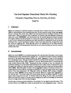
where θm is the delay of the peak effect. Equation (3) is proportional to the density function of a normal random variable with mean θm and variance −1/(2 log αm ). It is also referred to as the radial kernel basis function, which is the most commonly used kernel function in local regression (Friedman, Hastie & Tibshirani, 2009, p. 212). Figure 1 shows the weight functions of geometric adstock and delayed adstock for the same value of αm . Other functional forms, such as the negative binomial density function used in Hanssens et al. (2003), can also achieve the purpose of modelling a delay in the peak effect.

2.2

Shape Effect

To model the shape effect of advertising, the media spend needs to be transformed through a curvature function. A candidate for such a curvature function is the Hill function, which has its origins in pharmacology (Gesztelyi et al., 2012; Hill, 1910), where it was used as an empirical receptor model. It provides a flexible functional form: Hill(xt,m ; Km , Sm ) =

1 , 1 + (xt,m /Km )−Sm

xt,m ≥ 0

(4)

where Sm > 0 is the shape parameter which is also referred to as slope, and Km > 0 is the half saturation point, because Hill(Km ) = 1/2 for any value of Km and Sm . As x goes to infinity, 3

0.8 0.4 0.0

adstock

0

5

10

15

lag Figure 1: Example weight functions for geometric and delayed adstock. The black line is geometric adstock with αm = 0.8; the red line is delayed adstock with the same αm and θm = 5.

the Hill function approaches 1. To allow different maximum effects for different media, we further multiply the Hill function with the regression coefficient β. Hence the shape transformation is given by βHill(x), which can be rewritten as βm Hillm (xt,m ) = βm −

Sm β Km m Sm m xSt,m + Km

.

(5)

A similar functional form is used in Jin, Shobowale, Koehler and Case (2012) to describe the relationship between unique reach1 and Gross Rating Points2 (GRPs) or impressions of a TV campaign: b R=a− , (6) G + b/a where R stands for reach and G stands for GRPs. It is straightforward to see that (6) has a functional form that is equivalent to that of βHill(x) when S = 1, by letting a = β, b = Kβ and G = x, although it is used in a different application and has a different interpretation. Here and in the next paragraph we drop the subscripts in Km , Sm and βm for convenience. As seen in Figure 2, for the same values of K and β, compared to S = 1 (black solid curve), the curve of S > 1 (red curve) is convex close to zero, resulting in an S shape; on the other hand, the curve of S < 1 (green curve) is more concave close to zero and flattens faster. With one additional parameter, βHill(x) is more flexible than the functional form of (6). However, we have noticed that the parameters of βHill are essentially unidentifiable in some scenarios. For example, when S = 1, within a finite range, the curve can be approximated very well with a curve constructed from a very different set of three parameters. This is illustrated with the black solid (K = 0.5, S = 1, β = 0.3) and dashed lines (K = 0.95, S = 0.748, β = 0.393) in Figure 2, which only diverge for x > 1. Another scenario is when K is outside the range of observed media spend, as shown with the blue 1

Reach is the number of people in the target audience reached by a campaign divided by the total size of the audience. 2 GRP is the number of impressions delivered to the target audience divided by the number of people in the target audience, multiplied by 100.

4

0.4

half saturation

0.2

0.3

beta 0.3 0.3925 0.3 0.3 0.8 1.144

0.0

0.1

beta * Hill

slope

0.5 1 0.95 0.748 0.5 2 0.5 0.5 1.5 2 2 1.867

0.0

0.5

1.0

1.5

x

Figure 2: Hill functions.

solid (K = 1.5, S = 2, β = 0.8) and dashed lines (K = 2, S = 1.867, β = 1.144). In this case, the observed spend is assumed to be in the range (0, 1), and the two curves are nearly identical within that range, but diverge outside it. The poor identifiability of the βHill function makes it very challenging to estimate the parameters well with any statistical method. Alternatively, we could fit a more parsimonious functional form, such as the one in (6), referred to as reach transformation hereafter, which is equivalent to fixing S = 1 in estimating the Hill function. In Sections 6 and 7, we show that in some scenarios the individual parameters of the βHill transformation are not estimated well even though the curves are estimated well. Besides the Hill function, other functional forms can also be used to model the shape effect, such as the sigmoid function (also referred to as the logistic function), or the integral of other probability distributions such as the normal distribution. Another alternative is monotonic regression splines. More work is needed to compare different functional forms and regression splines and to investigate whether they suffer from the identifiability issue as well, which is out of the scope of this paper.

2.3

Combining the Carryover and the Shape Effect

In order to combine the carryover effect with the shape effect, there are two possible approaches. We could first apply the adstock transformation to the time series of media spend, and then apply the shape transformation. An alternative way would be to reverse the order. If media spend in each time period is relatively small compared to the cumulative spend across multiple time periods, the shape effect in each time period is less obvious compared to that of cumulative media spend. In this case, we would prefer to apply the shape transformation after the adstock transformation. However, if the media spend is heavily concentrated in some single time periods with an on-and-off pattern, the latter choice might be preferable. In this paper we have chosen the former, which is more appropriate for our data sets.

5

In this paper, for simplicity, we assume there is no synergy effect between media, which may not be true in reality (Zhang & Vaver, 2017). Hence the media effects are additive. Let yt be the response variable at week t, which could be sales or log transformed sales. The response can be modeled by the following generic equation yt = τ +

M X

βm Hill(x∗t,m ; Km , Sm ) +

m=1

C X

γc zt,c + t ,

(7)

c=1

where x∗t,m = adstock(xt−L+1,m , . . . , xt,m ; wm , L) as shown in (1), τ is the baseline sales, γc is the effect of control variable zc and t is some white noise that is assumed to be uncorrelated with the other variables in the model and to have constant variance. It is assumed that there is a linear relationship between the control variables and the response. While we have proposed several functional forms for the adstock and shape transformations, other functional forms may also be considered. In Section 8, we illustrate how to compare different Bayesian models and choose the best model specification based on the data and prior knowledge.

3

Estimating the Bayesian Model

As mentioned in Section 1, we use the Bayesian approach to estimate the model in (7) in order to make use of prior knowledge accumulated in previous media mix models. The model in (7) can also be extended to a hierarchical Bayesian model and applied to multiple related media mix data sets, utilizing their common information and allowing for differences, as shown in Wang, Jin, Sun, Chan and Koehler (2017) and Sun, Wang, Jin, Chan and Koehler (2017). Let Φ denote the vector of parameters in the model in (7), X denote all the media variables, Z denote all the control variables, and y denote the vector of response values. The frequentist approach finds the most likely value of the parameters by maximizing the likelihood (MLE), as in ˆ = arg max L(y|X, Z, Φ), Φ

(8)

Φ

where L(y|X, Φ) is the log likelihood given the data and the parameters. Details about the variance of MLE and its asymptotic distribution can be found in Lehmann and Casella (1998, p. 449). On the other hand, Bayesian inference treats the model parameters as random variables and is based on the posterior distribution (likelihood) of the parameters given the data and the prior distribution π(Φ): p(Φ|y, X) ∝ L(y|X, Z, Φ)π(Φ). (9) If a single number is required as a summary result for a media channel, modelers usually use the mean, median or mode of the posterior distribution (9) of parameter in or derived from Φ. A credible interval, usually quantile based, can also be derived from the posterior distribution (Hartigan, 2012; Hoff, 2009), and provides a more informative summary of the model output. When the prior distribution is conjugate, the posterior distribution in (9) typically has an analytical form. But in many other cases, we rely on drawing random samples from the posterior distribution to make inference of the parameters. A popular sampling method is Gibbs sampling (Gelfand & Smith, 1990; S. Geman & D. Geman, 1984), which partitions the parameter vector and converts high dimension sampling into iteratively sampling low dimensional conditional distributions. Another 6

sampling method that has gained popularity recently is Hamiltonian Monte Carlo (HMC) (Hoffman & Gelman, 2014). To sample from the model in (7) with appropriate prior distributions, we implemented Gibbs sampling in C++ using the slice sampler in Neal (2003) and the BOOM library (Scott, 2016). We also implemented another sampler using STAN (Carpenter et al., 2016), a probabilistic programming language that lets users specify the log density functions and get Bayesian inference with HMC sampling. The potential high correlation between the transformation parameters in our model poses a special challenge to the STAN sampler. While it can finish within a reasonable time on a data set of a few hundred data points, it could take quite a few hours or even a couple of days on larger data sets of a few thousand data points. Our customized Gibbs sampler is much more efficient. In Section 5, we compare the running time of both samplers on a simulated data set. The codes to implement the STAN sampler can be found in the Appendix. Setting the priors of the parameters has important implications on the resulting posterior distributions, as discussed in Gelman (2006, p. 1634-1637). If the data has strong information content, priors with the same support3 result in similar posterior distributions. If the data does not have strong information to estimate a parameter, the prior has a large influence on the posterior distribution and in some cases the posterior distribution may look almost the same as the prior. By definition, the retention rate α is constrained on [0, 1) and should have a prior that is defined on [0, 1), such as a beta or uniform distribution. It could have an even smaller support than [0, 1) if there is strong prior knowledge about the value of the retention rate. Similarly, the delay parameter θ usually has a prior that is constrained on [0, L − 1], such as a uniform or scaled beta distribution. For S, a common prior is a gamma distribution with a positive mode. As discussed in Section 2, the parameters of the Hill transformation are essentially unidentifiable if K is outside the range of observed media spend. Although in this case we cannot extrapolate the response curve beyond the observed media spend, it can still be estimated well within the observed media spend using a prior on K that is constrained over the range of the observed media spend, as shown in the simulation studies in Section 7. For the regression coefficients βm , we usually use nonnegative priors such as half normal (normal distribution constrained to be nonnegative), since we believe the media effect is nonnegative. In Section 7 we discuss in more details how the choice of priors could impact the model estimates through simulation studies.

4

Attribution Metrics and Optimal Media Mix

4.1

ROAS and mROAS

Besides estimates of the parameters in the model, a user of media mix models is also interested in attribution metrics derived from the model, in particular the Return on Ad Spend (ROAS) and the marginal ROAS (mROAS). Although an overall ROAS and mROAS can be calculated across all media spend, of more interest is the per channel ROAS and mROAS, which also guides optimization of the media mix. Here we assume we can change the spend of one media channel without affecting the spend of any other channel. This may not be applicable in situations when one media channel could affect the demand and spend of another channel, as discussed in the simulation scenarios of Zhang and Vaver (2017). In this case, ROAS and mROAS need to be calculated for the channels 3

Support is the set of values at which the probability density is positive. Or more rigorously, the the smallest closed set whose complement has probability zero.

7

Post−change Period

4.5

5.0

5.5

6.0

Change Period

4.0

Sales and scaled media spend

Pre−change Period

40

60

80

100

Week

Figure 3: Illustration of ROAS calculation for one media channel taking into account carryover effect. Black lines are predicted weekly sales, and blue lines are scaled spend in the channel. Solid lines are from historical spend, while dashed lines are generated by setting the spend in the change period to zero.

whose spend are correlated together, but not on individual channels. While these metrics can be calculated over the entire period of the dataset, they can also be restricted to a selected time period, in order to reflect more current conditions or use a similar seasonality pattern as the future time period in which media budget allocation will be guided by media mix results. We describe calculation of the per media ROAS and mROAS in further detail below. ROAS is the change in revenue (or sales) per dollar spent on the medium; it is usually calculated by setting spend of the medium to zero in the selected time period and comparing the predicted revenue against that of the current media spend. This is illustrated in Figure 3, where the selected time period is between the second and the third vertical lines, referred to as the change period. The blue solid line is the scaled historical spend on the medium, and the black solid line is the predicted sales. The corresponding dashed lines are generated by setting the spend on this medium to zero in the change period. The total difference between the two time series of predicted sales (the black solid and dashed lines) is the change in revenue attributable to the spend in the change period. Due to media carryover effect, the two lines differ in the post-change period, and the difference should be included in the calculation of ROAS as well. Similarly, the difference between the two lines is small at the beginning of the change period because of media lagged effect. Media spend in the pre-change period affects the amount of difference at the beginning of the change period until its carryover effect dies down. Hence we usually set the pre- and post-change periods to be of the same length as the maximum duration of carryover effect, unless they are truncated by data availability. The predicted sales is the sum of the first three terms in (7), excluding the noise term. If a transformation of sales, such as log transformation, is used as the response variable in (7), a 8

corresponding inverse transformation should be applied to get the predicted sales. Let Yˆt denote the predicted sales, which depends on media X, control variables Z and parameters Φ. Since the variables that determine the two time series of sales (the black solid and dashed lines) only differ in the mth media channel, we abbreviate Yˆt as a function of the mth channel. Suppose the historical spend on the mth channel (the blue solid line) is denoted with xt,m , and the blue dashed line of spend change is denoted with x et,m . The predicted sales using historical spend (the black m ˆ solid line) is denoted with Yt (xt−L+1,m , . . . , xt,m ; Φ), and the black dashed line is denoted with Yˆtm (e xt−L+1,m , . . . , x et,m ; Φ). ROAS for the m-th media is calculated as P ˆm ˆ m xt−L+1,m , . . . , x et,m ; Φ) t0 ≤t≤t1 +L−1 Yt (xt−L+1,m , . . . , xt,m ; Φ) − Yt (e P ROASm = , t0 ≤t≤t1 xt,m

(10)

where (t0 , t1 ) is the change period. Note that the numerator includes the difference in both the change period and the post-change period. As the model in (7) is additive in media effects, ROASm does not depend on other media channels except the mth channel or on control variables. mROAS for the m-th medium is the additional revenue generated in spend, P by one-unitˆ increase m with regard to Y usually from the current spent level. It is the derivative of t0 ≤t≤t1 +L−1 t P t0 ≤t≤t1 xt,m . It can be calculated analytically for tractable models, or estimated numerically by perturbing the media spend by a small amount. How this small amount of spend change is distributed in the change period affects the calculation of mROAS. A simple way is to apply multiplicative change of, for example, 1%, to the media spend in the selected period. P ˆm ˆm ˜ ˜ t0 ≤t≤t1 +L−1 Yt (xt−L+1,m , . . . , xt,m ; Φ) − Yt (xt−L+1,m , . . . , xt,m ; Φ) P mROASm = , (11) 0.01 × t0 ≤t≤t1 xt,m ˜t,m is the same time series of spend as xt,m but increasing the spend in the change period where x by 1%. In the frequentist approach, the maximum likelihood estimate of Φ is plugged into (10) and (11) to calculate ROAS and mROAS. Similarly, in the Bayesian framework, the posterior samples of Φ are plugged into (10) and (11) to obtain posterior samples of ROAS and mROAS. As discussed in Section 3, the reader can use either the mean, or the median, or the credible interval of the posterior distributions of ROAS and mROAS as a summary result. It may be tempting to first obtain the mean or median of individual parameters in Φ, and plug them into (10) and (11) to get one-number summaries of ROAS and mROAS. This is not recommended and could produce wrong results because it does not account for the correlation of the parameters in Φ.

4.2

Optimizing the Media Mix

Media mix models are also used to find the optimal media mix that maximizes the revenue under a budget constraint in the selected time period. Suppose the total budget of all media in the change period (t0 , t1 ) is C, the optimal media mix for this period Xo = {xot,m , t0 ≤ t ≤ t1 , 1 ≤ m ≤ M } is obtained by P ˆ maximize (12) t0 ≤t≤t1 +L−1 Yt (xt−L+1,m , . . . , xt,m ; 1 ≤ m ≤ M ; Φ) P P subject to (13) t0 ≤t≤t1 1≤m≤M xt,m = C. 9

Since in the optimization the control variables do not change, we abbreviate Yˆt as a function of the media variables and the parameters. Similar as in the calculation of ROAS and mROAS, due to media carryover effects, the objective function (12) should include the predicted sales in the post-change period. For a given set of parameters Φ, this optimization problem can be solved with constrained optimization methods such as Lagrange multiplier methods (Bertsekas, 2014). Depending on the number of media channels and the length of the change period, it may involve many free parameters and could be challenging to solve numerically. To reduce the number of free parameters, we can fix the flight pattern of the media, and find the optimal total spend on each medium. For example, suppose the spend over the change period is assumed to be constant, let cm denote the total spend on the mth medium, the time series of spend is xt,m = cm /(t1 − t0 + 1), t0 ≤ t ≤ t1 . Hence the constraint in (13) becomes X cm = C, (14) 1≤m≤M

and the problem only involves m free parameters. Other flight patterns can also be used, such as multiplicative change to the historical spend. In the Bayesian framework, with multiple posterior samples of the parameters, there are two approaches to obtain the optimal mix. In the first approach, we change the objective function in (12) to be the average of total predicted sales across all posterior samples of Φ as in maximize

1 X J

X

Yˆt (xt−L+1,m , . . . , xt,m ; 1 ≤ m ≤ M ; Φj ),

(15)

1≤j≤J t0 ≤t≤t1 +L−1

where Φj is the jth sample of the parameters and there are J samples in total. We then solve the constrained optimization problem as usual and find the optimal mix Xo . In the second approach, we plug each posterior sample of Φ into the objective function in (12), which becomes X maximize Yˆt (xt−L+1,m , . . . , xt,m ; 1 ≤ m ≤ M ; Φj ), (16) t0 ≤t≤t1 +L−1

and get the optimal mix for the jth sample Xoj . As mentioned in Section 3, the user can use either the mean, or the median or the credible interval of the posterior distribution of the optimal mix to summarize it. The first approach provides a more stable estimate of the optimal mix, while the posterior distribution from the second approach shows the variation of the estimated optimal mix. The variation of the estimated optimal mix is very important and informs the user how much he should trust the model in guiding budget allocation. Both approaches are illustrated on a simulated data set in Section 5.2 and on a real media mix data set in Section 8. Although in these two examples optimization only involves two media channels, both approaches can be applied to optimizing a media mix of multiple channels.

5

Application to a Simulated Data Set

In this section we illustrate how to estimate the media mix model in (7) on a simulated data set generated from a model of the same class as described in (7). Here we use the delayed adstock transformation and the βHill transformation. Models specified with other transformations, such as 10

geometric adstock and reach curve transformations, can be estimated similarly. We also illustrate how to calculate ROAS and mROAS, and how to optimize the media mix under a constraint on total budget.

5.1

Simulation Setting and Prior Distributions

The simulated data set contains 2 years of weekly data, sales, three media and one control variable (price). Media variables are generated by adding white noise to a sinusoidal seasonality with one year as a period; the control variable is generated as an ARIMA time series. For each media, the spend is scaled to be from 0 to 1 for convenience. Table 1 contains the parameters used in the model in (7) to generate sales as the response variable. Here we assume no transformation is used on the response variable. Figure 4 shows the time series plots of the sales and the media spend. Due to the data generation mechanism, weekly spend of all media have the same marginal distribution. Figure 4d shows the histogram of weekly spend of Media 1, which is quite spread out from 0 to 1. The media variables are also very weakly correlated with a correlation of 0.09. (a) Media specific parameters

Parameter

Media 1

Media 2

Media 3

α θ K S β

0.6 5 0.2 1 0.8

0.8 3 0.2 2 0.6

0.8 4 0.2 2 0.3

(b) Other variables

Parameter

Value

L τ γ 

13 4 -0.5 normal(0, 0.052 )

Table 1: Generating parameters.

Table 2 shows the signal strength of the media variables, price and the white noise, using the portion of the variance of sales explained as a strength metric. For example, for the m-th media, the strength metric is calculated as
Var βm Hill(x∗t,m ; Km , Sm ) . (17) Var(yt ) Due to the slight positive correlation between the media as shown in Figure 4e, the sum of the variances in Table 2 is less than 100%. This is expected since the variance of the sum of positively correlated variables is greater than the sum of the variance of the variables. The reader should focus on comparing the variance of the media against that of the white noise. Media 1 and media 2 have similar signal strength, while Media 3 is much weaker. The signal strength of this setting is similar as or stronger than that of most media mix data sets we have seen, which often suffer from high noise due to omitted variables and relatively small media impact (Chan & Perry, 2017). We use such a setting to better illustrate the model and how well it can be estimated. In Table 3 we list the priors used in estimating the model based on the simulated data set. They are chosen to contain the true parameter values, but with significant variance around the true values. More detailed discussion about the choice of priors can be found in Section 7. On a typical simulated data set, our Gibbs sampler with 10, 000 iterations took 52 seconds , while the STAN sampler with 1000 iterations took 1149 seconds. The posterior distribution of the regression coefficients and the transformation parameters can be found in Figure 18 in the Appendix. 11

(a) Sales

(b) Price

0.25

Price

Sales

5.4

5.2

0.00

−0.25

5.0

25

50

75

−0.50

100

25

50

Week

media.2

media.3

5 0

0.50

10

Frequency

0.75

0.25

0.0

0.2

0.4

0.6

0.00 25

50

media spend

75

Week

(e) Correlation of media and price

1

Correlation

0.01

0.5

price −0.1 0.18 0.01 media.3 0.17 0.16 media.2 0.11

1

1

0.16 0.18

1.0

0.0 −0.5

ic e

−1.0

pr

.3 ia

.2 ed

ia

.1 ed m

ia

0.11 0.17 −0.1

m

1

media.1

ed

0

m

Media Spend

15

media.1

100

(d) Histogram of weekly spend of Media 1

(c) Media spend media

75

Week

Figure 4: Sales, media and price in a typical simulated data set.

12

0.8

1.0

Media 1

Media 2

Media 3

Price

Noise

18.1%

19.4%

5.8%

22.5%

12.9%

Table 2: Variance of sales explained by media, price and noise.

Parameter

Prior

Parameter

Prior

α θ K S β

beta(3, 3) uniform(0, 12) beta(2, 2) gamma(3, 1) half normal(0, 1)

τ γ Var()

normal(0, 5) normal(0, 1) inverse gamma(0.05, 0.0005)

Table 3: Priors on parameters.

5.2

ROAS, mROAS and Optimal Media Mix

In calculating ROAS and mROAS, we assume the change period is one year, and the pre- and post-change periods are 12 weeks each, since L is assumed to be 13. The most recent 12 weeks are the post-change period, and one year prior to it is the change-period. This is illustrated in Figure 3 in Section 4.1, which is generated using this data set. The predicted sales are calculated using a randomly selected posterior sample of Φ. As described in Section 4.1, we obtain posterior samples of ROAS and mROAS by plugging posterior samples of Φ into (10) and (11), and use posterior medians as one-number summaries of ROAS and mROAS. In Figure 5, the black curves are the posterior density of ROAS and mROAS, the black dashed lines are the posterior medians, and the red lines are the true ROAS or mROAS. ROAS and mROAS of Media 2 are estimated reasonably well. ROAS of Media 1 has a bigger bias than that of Media 2, although its mROAS is estimated similarly well as Media 2. For Media 3, ROAS has very large extreme values, and mROAS has a large bias. We will show in Section 6 that the estimated βHill curves of Media 2 have the smallest bias among the curves of all three media. This explains why ROAS and mROAS of Media 2 are estimated better than the other two media. In this example, we aim to find the optimal media mix over a change period of 8 weeks, with the same pre- and post-change periods as mentioned above. For simplicity, the optimization only involves Media 1 and Media 2, and the spend of Media 3 is fixed at its historical values. As described in Section 4.2, to reduce the number of free parameters, we assume the weekly spend is constant during the change period. Hence the constraint on the total budget over the change period is equivalent to a constraint on the total weekly budget of Media 1 and Media 2. We consider two scenarios. In the first scenario, the total weekly budget is 1, and in the second scenario it is 0.5. We apply both approaches described in Section 4.2 to find the optimal mix under the budget constraint. In Figure 6a, the blue vertical lines are the optimal spend on Media 1 using the first approach, and the black curves are the posterior density of the optimal spend using the second approach. In Scenario I, both the blue line and the posterior median from the second approach (the black vertical line) are very close to the true optimal spend (the red line). In Scenario II, they are both

13

(a) ROAS media.1

media.2

media.3

2.0

density

2.0 1.5

0.9

1.0

0.6

0.5

0.3

0.0

0.0

1.5 1.0

0.5

1.0

1.5

2.0

0.5 0.0 1

2

3

4

0

1

2

3

4

value

(b) mROAS

density

media.1

media.2

media.3

10.0

10.0

7.5

7.5

5.0

5.0

5.0

2.5

2.5

2.5

0.0

7.5

0.0 0.3

0.4

0.5

0.6

0.0 0.4

0.5

0.6

0.7

0.0

0.1

0.2

0.3

value

Figure 5: Posterior distributions of ROAS and mROAS. In each plot, the black curve is the posterior density; the dashed line is the posterior median; the red line is the truth.

slightly off the true optimal spend. Figure 6b1 shows the estimated sales as the spend on Media 1 varies but the total spend is fixed. The black curves are calculated using individual posterior samples, which are the objective function in (16) in the second optimization approach. The blue curve is the average of the black curves, and is the objective function in (15) in the first approach. The red curve, calculated using the true model parameters in Table 1, represents the sales expected in reality. In Scenario I, most of the black curves peak around the true optimal spend, hence the posterior density is unimodal around the true optimal mix. In Scenario II, some black curves peak at the left end, and others peak near the right end. Hence the posterior density in Figure 6a2 has three modes. This shows that the estimated optimal mix in Scenario II has much higher variation than that in Scenario I, and is less trustworthy. In Scenario I, the fixed total weekly budget is close to the average weekly spend on Media 1 and Media 2 combined. In Scenario II, with half the total budget in Scenario I, sales are predicted in the more sparse part of observed data. Hence sales are not estimated as well as in Scenario I. The user of the model should be cautious when using the estimated optimal mix in scenarios such as the second one, since the variance in estimated sales is comparable or even larger than the variation in sales caused by different media mix.

6

Impact of Sample Size on Estimation Accuracy

Results shown in Section 5 are based on one simulated data set. Due to randomness in the data, it is hard to evaluate the model based on its performance on a single data set. In this section, we 14

(a) Optimal spend on Media 1 (a1) Total budget = 1

(a2) Total budget = 0.5 12

8 9

density

density

6

4

6

3

2

0

0 0.00

0.25

0.50

0.75

1.00

0.0

0.1

media spend

0.2

0.3

0.4

0.5

0.4

0.5

media spend

(b) Estimated Sales (b1) Total budget = 1 45 40 30

35

expected sales

40 35 30

expected sales

45

(b2) Total budget = 0.5

0.0

0.2

0.4

0.6

0.8

1.0

0.0

spend on Media 1

0.1

0.2

0.3

spend on Media 1

Figure 6: Posterior distributions of optimal spend on Media 1 and predicted sales at optimal mix. In the top panel, the red lines are the true optimal spend on Media 1. The blue vertical line is the optimal spend on Media 1 using the first optimization approach. The black curves are the posterior density of optimal spend on Media 1, using the second optimization approach, and the black vertical line is its posterior median. In the bottom panel, the red curves are the true expected sales, as the spend on Media 1 varies but the total spend over Media 1 and Media 2 is fixed. The black curves are the estimated sales using individual posterior samples, and the blue curve is the average of the black curves.

15

present results that are based on repeating the estimation procedure in Section 5 on 500 simulated data sets, each generated with a different random seed following the same model as in Section 5. For each data set, we calculate the medians of the posterior distributions of the parameters and the response curves βHill , and compare the mean of these medians to the true parameter values to assess if the model produces biased estimates for finite samples. We use the median of the posterior distribution rather than the mean because the mean is more sensitive to skewed distributions, which occur quite often in our example. We use the same simulation setting as in Section 5, but change the sample size to study its impact on the bias and variance of posterior medians. In the first scenario, each simulated data set contains two years of weekly data, while in the second scenario each data set contains sixty years of weekly data. In both scenarios the prior distributions are the same as in Table 3. Figure 7 shows the density of the posterior medians of the transformation parameters and the regression coefficients β over 500 data sets, with black curves representing the small sample size scenario and the light blue curves representing the large sample size scenario. Figure 8 shows the posterior medians of the βHill curves, which were plotted with the R package boom (Scott, 2016) and darker areas indicate higher density. Table 4 shows the relative difference of the mean of the posterior medians of βHill at x = 0.5 and 1 from the truth. x Sample Size Media 1 Media 2 Media 3

0.5 Two Years Sixty Years -39.7% -25.6% -39.0%

-0.2% 3.4% 10.4%

1 Two Years

Sixty Years

-32.5% -18.1% -25.3%

-0.2% 3.3% 10.4%

Table 4: Relative bias of βHill curves at x = 0.5 and x = 1.

In Figures 7a and 7b, the adstock parameters are estimated better for Media 1 and 2 than for Media 3, which has a weaker effect. The estimates of delay parameter θ have low bias and moderate uncertainty for all three media even in the small sample size scenario; in the large sample size scenario, they are almost unbiased and have very small variance. Estimates of α exhibit somewhat more bias and uncertainty for small sample size, but are again precise and accurate for large sample size. Estimating the parameters of the shape transformation is much harder, as seen in Figures 7d, 7c, and 7e. Even in the large sample size scenario, while the bias is low, the posterior medians of K, S and β vary widely; in the small sample size scenario, they are subject to high variance and large bias. The βHill curves for all media are underestimated for the small sample size, as shown in Figure 8a. Media 1 has the largest bias of all three, even though it has similar signal strength as Media 2. This is because the true value of S is 1 for Media 1, which makes the shape transformation less identifiable, as explained in Section 2. In Figure 8b, for the large sample size, all response curves are estimated very well, with very low bias and small variance. Due to the near unidentifiability of the βHill function discussed in Section 2, although the response curve can be estimated well, the individual shape parameters are very hard to estimate well, as discussed earlier. The bias seen in the small data set can be attributed to the prior distributions. When the sample 16

(a) Retention rate α

density

media.1

media.2

media.3 20

30

20

15 20

10

10 10 0

5

0 0.4

0.6

0.8

0 0.5

0.6

0.7

0.8

0.9

0.4

0.6

0.8

value

(b) Delay θ

media.1

media.2

media.3

density

6 10

1.5

4

5

1.0

2

0

0.5

0 4.4

4.8

5.2

5.6

0.0 2.0

2.5

3.0

3.5

4.0

4.5

0

3

6

9

value

(c) Slope S

media.1

media.2

2.0

density

media.3

1.5 0.9

1.5

1.0

0.6

1.0 0.5

0.5 0.0

0.3

0.0 1

2

3

0.0 1

2

3

4

1

2

3

4

5

value

(d) Half saturation K

density

media.1

media.2

media.3

12

20

12

9

15

9

6

10

6

3

5

3

0

0 0.2

0.4

0.6

0.8

0 0.2

0.4

0.6

0.0

0.2

0.4

0.6

0.8

value

Figure 7: Density of posterior medians over 500 data sets. The black curves are for sample size of two years, while the light blue curves are for sample size of sixty years. The dashed vertical lines are the mean of the posterior medians, and the red vertical line indicates the true value.

17

(e) Regression coefficients β

media.1

media.2

3

density

media.3 5

5

2 1 0

4

4

3

3

2

2

1

1

0 0.5

1.0

0.2

0.4

0.6

0.8

1.0

0 0.00

0.25

0.50

0.75

value

Figure 7: Density of posterior medians over 500 data sets (continued).

(a) Two years

0.0

0.2

0.4

0.6

0.8

1.0

0.4 0.1 0.0

0.0

0.0

0.1

0.2

0.2

0.2

0.3

0.4

0.4

0.3

0.5

0.6

0.6

0.5

media 3

0.7

media 2

0.8

media 1

0.0

0.2

Media Spend

0.4

0.6

0.8

1.0

0.0

0.2

Media Spend

0.4

0.6

0.8

1.0

0.8

1.0

Media Spend

(b) Sixty years

0.0

0.2

0.4

0.6

Media Spend

0.8

1.0

0.4 0.1 0.0

0.0

0.0

0.1

0.2

0.2

0.2

0.3

0.4

0.4

0.3

0.5

0.6

0.6

0.5

media 3

0.7

media 2

0.8

media 1

0.0

0.2

0.4

0.6

Media Spend

0.8

1.0

0.0

0.2

0.4

0.6

Media Spend

Figure 8: Posterior medians of βHill curves over 500 data sets using different sample sizes. In each plot, a black or grey line is the posterior median of βHill curves on one simulated data set. Each plot contains 500 such curves. The red line is the true βHill curve, and the blue line is the mean of the posterior medians represented by the black and grey lines.

18

size is small and the signal is weak, the posterior distribution is mostly determined by the priors. Hence the data is not strong enough to correct any bias introduced by the priors. The actual sample size required for the estimates to be unbiased vary for different scenarios. In the next section we discuss in more detail how priors can change the posterior distributions. In this simulated example we increase the sample size by including data over a much longer historical period. However, this is not the recommended way to increase sample size in real problems, as other factors such as market demand and macroeconomic factors would have changed significantly over a prolonged time period. In Section 9 we discuss other approaches to increase the sample size and gather more powerful data.

7

Choice of Priors

As mentioned in Section 3, when the sample size is small, the priors have a large influence on the posterior distributions. Here we study the difference in the posterior distributions from using different priors. We focus on the priors for β and K.

7.1

Prior on β

We use three different priors on β: half normal(0, 1), normal(0, 1) and uniform(0, 3). The simulation setting is the same as in Section 5, and is repeated on 500 simulated data sets. Figure 9 shows the density of posterior medians of β, and Table 5 reports the relative bias of βHill curves using different priors. To save space, we only show the posterior medians of βHill curves for Media 2 in Figure 10. Figure 10a is the same plot as Figure 8a; it is repeated here for the reader to compare with the curves of other priors conveniently.

media.1

media.2

density

3

media.3 4

3

2

Prior on Beta

3

half normal(0, 1)

2

normal(0, 1)

1

uniform(0, 3)

2

1

1

0

0 0.4

0.8

1.2

0 0.5

1.0

0.0

0.5

1.0

1.5

value

Figure 9: Posterior medians of β over 500 data sets using different priors on β. The dashed lines are the mean of the posterior medians of β, and the red lines are the truth.

The estimates of β and βHill produced with half normal(0, 1) and normal(0, 1) as priors are very similar, and both are very different from those of using uniform(0, 3) as the prior. As seen in Table 5, using uniform(0, 3) as the prior on β, the βHill curves have smaller bias compared to using the other two priors. This is because uniform(0, 3) puts more mass on larger values of β than the other priors, which helps with correcting the underestimated curves. But this cannot be generalized to claim that uniform(0, 3) is a more appropriate prior because in other scenarios the response curves

19

x Prior on β

half normal

0.5 normal

uniform

half normal

1 normal

uniform

Media 1 Media 2 Media 3

-39.6% -25.5% -39.3%

-39.4% -25.6% -42.2%

-27.7% -4.5% -22.6%

-32.4% -18.0% -25.6%

-32.3% -18.0% -28.7%

-21.7% -1.5% -10.3%

Table 5: Relative bias of βHill curves at x = 0.5 and x = 1 using different priors on β.

0.0

0.2

0.4

0.6

0.8

1.0

0.4 0.0

0.2

0.4 0.2 0.0

0.0

0.2

0.4

0.6

(c) Uniform(0, 3)

0.6

(b) Normal(0, 1)

0.6

(a) Half normal(0, 1)

0.0

Media Spend

0.2

0.4

0.6

0.8

1.0

Media Spend

0.0

0.2

0.4

0.6

0.8

1.0

Media Spend

Figure 10: Posterior medians of βHill curves for Media 2 over 500 data sets using different priors on β.

may be over-estimated, and using uniform(0, 3) will make the bias bigger compared to the other two priors.

7.2

Prior on half saturation K

We consider two scenarios with different true values of K. In Scenario I, we use the same simulation setting as in Section 5, with K = 0.2 for all media. In Scenario II, the simulation setting is similar, but K is 2 for all media and the regression coefficients β for the three media are 2, 3, 1.5 respectively. Since the observed media spend in our simulator ranges from 0 to 1, K is within the observed range of media spend in Scenario I, but is outside the observed range in Scenario II. We use three different priors on K: beta(2, 2), uniform(0, 1), and uniform(0, 10). To save space, we only report posterior medians of K for Media 2 in Figure 11, the posterior medians of βHill curves for Media 2 in Figure 12 and its relative bias in Table 6. x Prior on K Scenario I Scenario II

beta(2, 2)

0.5 uniform(0, 1)

uniform(0, 10)

-25.5% -0.7%

-16.0% -0.6%

-21.2% -8.9%

beta(2, 2)

1 uniform(0, 1)

uniform(0, 10)

-18.0% -25.2%

-9.2% -21.2%

-10.2% -13.6%

Table 6: Relative bias of posterior medians of βHill curves for Media 2 at x = 0.5 and x = 1 using different priors on K.

20

Half saturation = 0.2

Half saturation = 2 5

density

4

Prior on half saturation K

4

3 2 1

3

beta(2, 2)

2

uniform(0, 1) uniform(0, 10)

1

0

0 0

1

2

3

0

1

2

3

Figure 11: Posterior medians of K for Media 2 over 500 data sets using different priors on K. The dashed lines are the mean of the posterior medians of K, and the red lines are the truth. (a) True value of K = 0.2 (a2) uniform(0, 1)

0.0

0.2

0.4

0.6

0.8

1.0

0.6 0.4 0.2 0.0

0.2

0.4

0.6

(a2) uniform(0, 10)

0.0

0.0

0.2

0.4

0.6

(a1) beta(2, 2)

0.0

0.2

Media Spend

0.4

0.6

0.8

1.0

0.0

0.2

Media Spend

0.4

0.6

0.8

1.0

Media Spend

(b) True value of K = 2 (b2) uniform(0, 1)

0.0

0.2

0.4

0.6

Media Spend

0.8

1.0

0.6 0.4 0.2 0.0

0.2

0.4

0.6

(b2) uniform(0, 10)

0.0

0.0

0.2

0.4

0.6

(b1) beta(2, 2)

0.0

0.2

0.4

0.6

Media Spend

0.8

1.0

0.0

0.2

0.4

0.6

0.8

1.0

Media Spend

Figure 12: Posterior medians of βHill curves for Media 2 over 500 data sets using different priors on K.

As shown in Figure 12, in both scenarios, the three priors produce very similar estimates of βHill curves. However, the estimates of K are similar between the first two priors, but are quite different from those of the third prior, shown in Figure 11. In Scenario I, the posterior medians of K using the third prior have a larger bias than those using the other two priors, while in Scenario II it is

21

the opposite. In both scenarios, there is less variation in the posterior medians of K using the first two priors than the third prior. Since media effect depends on the βHill curve, not its individual parameters, the model is not very sensitive in the choice of prior on K. However, a tighter prior is still preferred if it is supported by prior knowledge, since it would make the sampler converge faster. In Scenario II, due to K being nearly unidentifiable beyond the observed data range, as discussed in Section 2, even with a prior that has probablity mass over the true value of K, such as uniform(0, 10), the model still cannot estimate K well. It is also interesting to note that even though K is not estimated well, the βHill curves are estimated quite well within the observed data range in Scenario II.

8

Application to Real Data and Model Selection

We apply the media mix model in (7) to data of a shampoo advertiser, provided by Neustar MarketShare. The data was consolidated from sources such as Kantar Media, IRI, ITG, JD Power, and Rentrak. It contains 2.5 years of weekly data, including weekly volume sales in ounces and media spend on major channels such as TV, magazines, display, YouTube, and search. Also available are retailer variables such as the average price per ounce, ACV4 weighted product distribution, and ACV weighted promotions. We use log transformed volume sales as the response variable y, and the three merchant variables mentioned above as the control variables, referred to as price, distribution and promotion. We fit four models on the five media channels mentioned above, with different choices of adstock and shape transformations as described in Table 7. Model I is the most complicated, while Model IV is the most parsimonious. Model

Adstock Transformation

Shape Transformation

I II III IV

delayed adstock delayed adstock geometric adstock geometric adstock

βHill reach βHill reach

Table 7: Specification of adstock and shape transformations in the four models.

The models are estimated with the STAN sampler, using similar priors as in Table 3 in the simulation studies. Table 8 shows the running time of STAN for each of the four models. Model I, the most complicated model, takes much longer than the more parsimonious models. The control variables are highly correlated, as shown in Figure 13a, which induces high correlation in the posteriors of the regression coefficients γc , c = 1, . . . , 3. Including them directly in the model would cause the MCMC sampler to take a much longer time to converge. Instead, we make them nearly orthogonal by regressing each of distribution and promotion onto price and use the residuals of the single variate linear regression as a predictor in the model. As shown in the first two rows of Table 8, with only two major media channels TV and magazines, using the original control 4

ACV is short for all-commondity volume, which is a weighted measure of product availability, or distribution, based on total store sales.

22

Model

Control

Media

Running Time in Seconds

I I I II III IV

Original Correlated Variables Orthogonal Variables Orthogonal Variables Orthogonal Variables Orthogonal Variables Orthogonal Variables

TV, Magazines TV, Magazines all five media all five media all five media all five media

3040 75 471 181 112 91

Table 8: Running time of the STAN sampler in training the four models. Each model is trained by running three chains in parallel in STAN, with 1000 iterations each. The running time shown here is that of the chain that finished last. All models converged well, with the Gelman-Rubin potential scale reduction factor ˆ (Gelman & Rubin, 1992) equal to or close to 1. R

variables, the STAN sampler took 3040 seconds; using the predictors that are made orthogonal, the sampler only took 75 seconds. (b) Media spend (a) Control search Correlation

promotion −0.77 0.74

1

YouTube

1.0

1

0.74

0.05 −0.04 0.17

1

1 −0.23

Correlation 1.0 0.5

0.5

distribution −0.98

0.46 0.11 −0.15 −0.23

display

0.28 0.21

1

0.17 −0.15

0.0

0.0 −0.5

1 −0.98−0.77

price

magazines

−0.5

0.13

1

0.21 −0.04 0.11

−1.0

h ar c se

ne s az i

m

ag

la y Yo uT ub e

0.13 0.28 0.05 0.46

tv

1

di sp

io pr n om ot io n

tv

rib ut

di

st

pr

ic e

−1.0

Figure 13: Correlation of control and media variables.

We use Bayesian Information Criterion (BIC) (Schwarz, 1978) to select the most appropriate model for this data set. BIC = −2 log Lˆ + k log(n), (18) where Lˆ is the maximized value of the likelihood function, k is the number of free parameters, and n is the sample size. log Lˆ is approximated by the average of the log likelihood plugging in the posterior samples of the parameters after the MCMC sampler has burned in5 . BIC balances the need of fitting the data well and penalizing against model complexity. In general we prefer a model with the smallest BIC value. Other model selection criteria such as DIC (Spiegelhalter, Best, Carlin & Van Der Linde, 2002) or WAIC (Vehtari, Gelman & Gabry, 2015; Watanabe, 2010) can also be used. However, the reader should bear in mind that these criteria aim at selecting the most appropriate regression model, not the model with the most accurate causal inference. As shown in Table 9, the maximum log likelihood of the four models are very similar. Hence BIC favors the most parsimonious model, Model IV. 5

We set the first half of the iterations per chain as burn-in iterations, which is the default setting in STAN

23

Model

Negative Log Likelihood

Change in k

Change in Penalty6

BIC7

I II III IV

98.12 98.11 98.06 98.09

0 -5 -5 -10

0 -23.3 -23.3 -46.6

98.12 74.81 74.76 51.49

Table 9: BIC values of the four models.

In Figure 14 we report ROAS and mROAS of the two largest spending channels of this advertiser, TV and magazines. The values of ROAS and mROAS of the two channels are scaled by a common constant. The four models produce similar estimates of mROAS of TV (the top right figure) and ROAS of magazines (the bottom left figure). Model II and Model IV (the blue and the red lines), which use reach transformation, have smaller posterior medians of mROAS of magazines than the other two models. For ROAS of TV, it is the opposite, although the difference in posterior medians of the four models is smaller compared to that for mROAS of magazines. All models have large extreme values in the posterior distributions of ROAS. The posterior distributions of mROAS have similar long right tails for all the models except Model IV, which has the least variance of mROAS for both TV and magazines. Using Model IV, we carry out both approaches of optimization involving TV and magazines. It assumes the total weekly spend on the two channels is at its historical average. Figure 15a shows that the posterior distribution of the optimal spend on TV has two modes at the extreme ends of the spend range. In Figure 15b, the estimated sales have much larger variation across posterior samples than across different media mix. As described in Section 5.2, the estimated optimal mix is not trustworthy in this scenario. If we set the fixed total weekly spend to be very different from its historical average, the estimated sales will have even larger variance because they are predicted either in the sparse part of the observed data or after extrapolating the data. In Figure 16 we report the posterior distributions of βHill curves and the parameters of the adstock transformation for TV. The βHill curves are plotted against scaled media spend. The reader should note that the scale of the y axis in the βHill curves for Models I and III (Figures 16a3 and 16c2) is 20 times as large as that for Models II and IV (Figures 16b3 and 16d2). In Models I and III, which use the Hill transformation, the credible interval of βHill is much wider than that of Models II and IV, which use the reach transformation. Allowing a more flexible functional form of curvature does not lead to more accurate estimates, instead, it results in much larger variance. The delay parameter θ is not estimated well in either Model I or Model II. Hence we would prefer the simpler adstock transformation, geometric adstock. Finally, the posterior distribution of retention rate α (black curve) is almost the same as the prior (orange curve), which indicates the data does not have enough information to alter the prior belief. As illustrated with the simulation studies in Section 6, it is usually difficult to estimate the shape and the adstock transformations well if the data consist of only a few hundred observations. The prior distributions on the parameters largely determine the posterior distributions, as shown in this example, and may lead to biased estimates if they are not chosen properly. In the next section, we discuss other approaches to gather a more powerful data set to estimate the transformation 6 7

n = 106 BIC values here are different from the one calculated in (18) by a constant common to all models.

24

(a) TV

ROAS

mROAS

15 7.5

density

Model Model I

10 5.0

Model II Model III

5

2.5

0

Model IV

0.0 0.0

0.2

0.4

0.6

0.0

0.2

0.4

0.6

(b) Magazines

ROAS

mROAS

12

density

9

Model

10

Model I Model II

6

Model III

5

Model IV

3

0

0 0.0

0.2

0.4

0.6

0.0

0.2

0.4

0.6

Figure 14: Posterior distributions of scaled ROAS and mROAS of TV and magazines using the four models. The dashed lines are the posterior medians of ROAS or mROAS for each model. (a) Optimal spend on TV

100

(b) Estimated sales as the spend on TV varies

density

60

10

40

scaled sales

80

15

0

20

5

0 0

0.2

0.4

0.6

0.8

0.0

1

ratio of spend on TV over total spend

0.2

0.4

0.6

0.8

1.0

ratio of spend on TV over total spend

Figure 15: Optimal budget allocation between TV and magazines under a constraint on total budget, using Model IV. On the left plot, the blue line is the optimal spend on TV using the first optimization approach. The black curve is the posterior density of the optimal spend on TV using the second approach described, and the black vertical line is the posterior mean. On the right plot, the black and grey curves are the estimated sales calculated with individual samples, when the spend on TV varies but the total budget on TV and magazines is fixed. The blue curve is the average of the black and grey curves. The blue and black vertical lines correspond to those on the left plot. Both spend on TV and the estimated sales are scaled.

25

(a) Model I: Delayed adstock and Hill transformation (a3) βHill

(a2) Delay θ 0.6

(a1) Retention rate α

0.5

2.5 0.15

0.3

0.4

1.0

0.10

0.2

1.5

density

density

2.0

0.1

0.05

0.0

0.5 0.0

0.00 0.00

0.25

0.50

0.75

1.00

0.0

0

value

5

0.2

10

0.4

0.6

0.8

1.0

0.8

1.0

Scaled Media Spend

value

(b) Model II: Delayed adstock and reach transformation (b3) βHill

(b2) Delay θ 0.030

(b1) Retention rate α

2.0

0.020

0.09

1.0

0.06 0.010

density

density

1.5

0.03 0.000

0.5

0.0

0.00 0.00

0.25

0.50

0.75

1.00

0.0

0

value

5

0.2

10

0.4

0.6

Scaled Media Spend

value

(c) Model III: Geometric adstock and Hill transformation (c1) Retention rate α 0.6

(c2) βHill

0.4

0.5

2.0

0.3 0.2

1.0

0.1

density

1.5

0.0

0.5 0.0 0.00

0.25

0.50

0.75

0.0

1.00

value

0.2

0.4

0.6

0.8

1.0

Scaled Media Spend

Figure 16: Posterior distributions of βHill curves and the parameters in the adstock transformation of the four models. The black lines are the posterior density of the parameters, and the orange lines are the density of the prior distributions. The blue dashed lines are the 95% credible intervals and the medians of the βHill curves.

26

(d) Model IV: Geometric adstock and reach transformation (d1) Retention rate α 0.030

(d2) βHill

0.020

1.5

0.010

density

2.0

1.0

0.000

0.5

0.0 0.00

0.25

0.50

0.75

0.0

1.00

0.2

value

0.4

0.6

0.8

1.0

Scaled Media Spend

Figure 16: Posterior distributions of βHill curves and the parameters in the adstock transformation of the four models (continued).

parameters. For each MCMC draw of posterior samples of the parameters, we compute the autocorrelation of the residuals of the regression model. Figure 17a shows the average autocorrelation across all MCMC draws. Compared to the autocorrelation of the response variables in Figure 17b, the residuals are much less auto-correlated. This shows that through the explanatory variables and the adstock transformation, the model explains a large part of the autocorrelation of the response variable. However, there is still significant autocorrelation in the residuals up until a lag of 15 weeks, which is a sign of model misspecification. (a) Average autocorrelation of residuals across all MCMC iterations

−0.2

0.4

ACF

0.4 −0.2

ACF

1.0

1.0

(b) Autocorrelation of log transformed sales

0

5

10

15

0

20

5

10

15

20

Lag

Lag

Figure 17: Autocorrelation of residuals and sales.

9

Conclusion

Media mix models can vary greatly in their model specification. In this paper, we propose a media mix model with flexible functional forms for media carryover and shape effects and show how the model parameters can be estimated in a Bayesian framework. Attribution metrics such as ROAS, mROAS and optimal mix can also be calculated using the posterior samples of the parameters. 27

Large scale simulation studies show that the model can be estimated well on a large data set, but it may produce biased estimates for the typical sample size of a couple of years of weekly national-level data. In this case, the prior distributions have a large impact on the posterior distributions, and different priors may result in quite different posterior distributions and lead to different attribution metrics. Therefore, in order to estimate the model well and get accurate attribution, it is very important to gather more powerful data sets and use more informative priors. This point is further illustrated on a shampoo advertiser data, which does not have enough information content to estimate the carryover and shape effects well. We use BIC as the model selection criteria and select the most parsimonious functional form for the adstock and the shape transformations. We report scaled ROAS and mROAS values of TV and magazines and conduct optimization of the two channels under a fixed total budget. The predicted sales have much smaller variation across different media mix than that caused by the variance in the model estimates. To derive more informative priors, Wang et al. (2017) pools data of similar brands within one category, and extends the flat model in (7) to a hierarchical Bayesian model that allows random effects of media and control variables for different brands. Sun et al. (2017) uses geo-level data instead of national-level data to estimate a similar hierarchical Bayesian model with the shape and the adstock transformations. In simulations, both approaches estimate the transformation parameters well with a much larger data set and derive informative priors to use when the model is applied to a single brand nation-level only data. As shown with the diagnostic analysis of the residuals of the example in Section 8, the regression model in (7) may not capture all the autocorrelation of the response variables. The model can be extended to a multi-stage regression or graphical model to allow for a more complex mechanism of media’s impact on sales. Similarly, the simulator we used to study the statistical properties of the model is a simplification of how data is generated in reality. Zhang and Vaver (2017) introduces a simulator which takes into account media synergy effects. It could be used to evaluate how the model proposed here performs on more realistic media mix data sets.

Acknowledgment We would like to thank Tony Fagan and Penny Chu for their encouragement and support, Wiesner Vos, Steve Scott, Bob Bell and Michael Perry for very constructive comments which greatly improved the paper, Jon Vaver, Stephanie Zhang, Zhe Chen, Aiyou Chen, Shi Zhong, Conor Sontag, Felipe Gonzalez, and Xiaojing Huang for insightful discussions.

Appendix STAN Sampler Codes Below is the STAN file that specifies the media mix model, assigns priors and estimates it on the simulated data set in Section 5. functions { // the Hill function real Hill(real t, real ec, real slope) { 28

return 1 / (1 + (t / ec)^(-slope)); } // the adstock transformation with a vector of weights real Adstock(row_vector t, row_vector weights) { return dot_product(t, weights) / sum(weights); } } data { // the total number of observations int N; // the vector of sales real Y[N]; // the maximum duration of lag effect, in weeks int max_lag; // the number of media channels int num_media; // a vector of 0 to max_lag - 1 row_vector[max_lag] lag_vec; // 3D array of media variables row_vector[max_lag] X_media[N, num_media]; // the number of other control variables int num_ctrl; // a matrix of control variables row_vector[num_ctrl] X_ctrl[N]; } parameters { // residual variance real noise_var; // the intercept real tau; // the coefficients for media variables vector[num_media] beta_medias; // coefficients for other control variables vector[num_ctrl] gamma_ctrl; // the retention rate and delay parameter for the adstock transformation of // each media vector[num_media] retain_rate; vector[num_media] delay; // ec50 and slope for Hill function of each media vector[num_media] ec; vector[num_media] slope; } transformed parameters { 29

// a vector of the mean response real mu[N]; // the cumulative media effect after adstock real cum_effect; // the cumulative media effect after adstock, and then Hill transformation row_vector[num_media] cum_effects_hill[N]; row_vector[max_lag] lag_weights; for (nn in 1:N) { for (media in 1 : num_media) { for (lag in 1 : max_lag) { lag_weights[lag] <- pow(retain_rate[media], (lag - 1 - delay[media]) ^ 2); } cum_effect <- Adstock(X_media[nn, media], lag_weights); cum_effects_hill[nn, media] <- Hill(cum_effect, ec[media], slope[media]); } mu[nn] <- tau + dot_product(cum_effects_hill[nn], beta_medias) + dot_product(X_ctrl[nn], gamma_ctrl); } } model { retain_rate ~ beta(3,3); delay ~ uniform(0, max_lag - 1); slope ~ gamma(3, 1); ec ~ beta(2,2); tau ~ normal(0, 5); for (media_index in 1 : num_media) { beta_medias[media_index] ~ normal(0, 1); } for (ctrl_index in 1 : num_ctrl) { gamma_ctrl[ctrl_index] ~ normal(0,1); } noise_var ~ inv_gamma(0.05, 0.05 * 0.01); Y ~ normal(mu, sqrt(noise_var)); }

30

(a) Regression coefficient β

media.1

media.2

media.3

density

2.0 1.0

3

1.5 1.0

2

0.5

1

0.5 0.0

0.0 0

1

2

3

0 0

1

2

3

0.0

0.5

1.0

1.5

2.0

value

(b) Retention Rate α

density

media.1

media.2

4

media.3

8

2.0

6

1.5

4

1.0

2

0.5

2 0 0.4

0.6

0.8

0 0.5

0.0 0.6

0.7

0.8

0.9

0.00

0.25

0.50

0.75

1.00

value

(c) Delay θ

media.1

media.2

density

3

media.3 0.6

2.0 1.5

2

0.4

1.0 1

0.2

0.5

0 4.5

4.8

5.1

5.4

0.0 5.7

0.0 3.0

3.5

4.0

0

4

8

12

value

Figure 18: Posterior distributions of regression coefficients, transformation parameters and response curves on one simulated data set.

31

(d) Half saturation K

media.1

media.2

2.5

media.3

6

1.5

4

1.0

2

0.5

density

2.0 1.5 1.0 0.5 0.0

0 0.00

0.25

0.50

0.75

1.00

0.00

0.25

0.50

0.75

0.0 1.00 0.00

0.25

0.50

0.75

1.00

value

(e) Slope S

media.1

media.2

media.3

0.6

0.8

density

0.3 0.6

0.4

0.2

0.4 0.2

0.2 0.0

0.1

0.0 0

1

2

3

4

5

0.0 0

2

4

6

0

4

8

12

value

(f ) βHill media 3

0.0

0.6 0.4 0.2

0.0

0.0

0.2

0.2

0.4

0.4

0.6

0.6

0.8

0.8

1.0

1.2

0.8

media 2

1.0

media 1

0.0

0.2

0.4

0.6

Media Spend

0.8

1.0

0.0

0.2

0.4

0.6

Media Spend

0.8

1.0

0.0

0.2

0.4

0.6

0.8

1.0

Media Spend

Figure 18: Posterior distributions of regression coefficients, transformation parameters and response curves on one simulated data set(continued).

32

References Bertsekas, D. P. (2014). Constrained optimization and lagrange multiplier methods. Academic press. Borden, N. H. (1964). The concept of the marketing mix. Journal of advertising research, 4 (2), 2–7. Carpenter, B., Gelman, A., Hoffman, M., Lee, D., Goodrich, B., Betancourt, M., . . . Riddell, A. (2016). Stan: a probabilistic programming language. Journal of Statistical Software, 20. Chan, D. & Perry, M. (2017). Challenges and opportunities in media mix modeling. research.google.com. Chen, A., Chan, D., Perry, M., Jin, Y., Sun, Y., Wang, Y. & Koehler, J. (2017). Bias correction for paid search in media mix modeling. Forthcoming on https:// research.google.com. Friedman, J., Hastie, T. & Tibshirani, R. (2009). The elements of statistical learning (2nd edition). Springer series in statistics Springer, Berlin. Gelfand, A. E. & Smith, A. F. (1990). Sampling-based approaches to calculating marginal densities. Journal of the American statistical association, 85 (410), 398–409. Gelman, A. (2006). Prior distribution. In Encyclopedia of environmetrics. John Wiley & Sons, Ltd. doi:10.1002/9780470057339.vap039 Gelman, A. & Rubin, D. B. (1992). Inference from iterative simulation using multiple sequences. Statistical science, 457–472. Geman, S. & Geman, D. (1984). Stochastic relaxation, gibbs distributions, and the bayesian restoration of images. IEEE Transactions on pattern analysis and machine intelligence, (6), 721– 741. Gesztelyi, R., Zsuga, J., Kemeny-Beke, A., Varga, B., Juhasz, B. & Tosaki, A. (2012). The Hill equation and the origin of quantitative pharmacology. Archive for History of Exact Sciences, 66 (4), 427–438. doi:10.1007/s00407-012-0098-5 Guadagni, P. M. & Little, J. D. (1983). A logit model of brand choice calibrated on scanner data. Marketing science, 2 (3), 203–238. doi:10.1287/mksc.2.3.203 Hanssens, D. M., Parsons, L. J. & Schultz, R. L. (2003). Market response models: econometric and time series analysis. Springer Science & Business Media. Hartigan, J. A. (2012). Bayes theory. Springer Science & Business Media. Hill, A. V. (1910). The possible effects of the aggregation of the molecules of haemoglobin on its dissociation curves. Journal of Physiology, 40 (suppl), iv–vii. doi:10.1113/jphysiol.1910. sp001386 Hoff, P. D. (2009). A first course in bayesian statistical methods. Springer Science & Business Media. Hoffman, M. D. & Gelman, A. (2014). The no-u-turn sampler: adaptively setting path lengths in hamiltonian monte carlo. Journal of Machine Learning Research, 15 (1), 1593–1623. Jin, Y., Shobowale, S., Koehler, J. & Case, H. (2012). The incremental reach and cost efficiency of online video ads over tv ads. research.google.com. Retrieved from https://research.google. com/pubs/pub40426.html

33

Lehmann, E. L. & Casella, G. (1998). Theory of point estimation. Springer Science & Business Media. McCarthy, J. E. (1978). Basic marketing: a managerial approach (6th ed.). Homewood, Il: R.D. Irwin. Neal, R. M. (2003). Slice sampling. The Annals of Statistics, 31 (3), 705–767. doi:10.1214/aos/ 1056562461 Rosenbaum, P. R. & Rubin, D. B. (1983). The central role of the propensity score in observational studies for causal effects. Biometrika, 70 (1), 41–55. Schwarz, G. (1978). Estimating the dimension of a model. The annals of statistics, 6 (2), 461–464. Scott, S. L. (2016). Boom: bayesian object oriented modeling. R package version 0.5. Spiegelhalter, D. J., Best, N. G., Carlin, B. P. & Van Der Linde, A. (2002). Bayesian measures of model complexity and fit. Journal of the Royal Statistical Society: Series B (Statistical Methodology), 64 (4), 583–639. Sun, Y., Wang, Y., Jin, Y., Chan, D. & Koehler, J. (2017). Geo-level bayesian hierarchical media mix modeling. research.google.com. Tellis, G. J. (2006). Modeling marketing mix. In R. Grover & M. Vriens (Eds.), Handbook of marketing research: uses, misuses, and future advances (pp. 506–522). Thousand Oaks, CA. doi:10.4135/9781412973380.n24 Vehtari, A., Gelman, A. & Gabry, J. (2015). Efficient implementation of leave-one-out crossvalidation and waic for evaluating fitted bayesian models. arXiv preprint arXiv:1507.04544. Wang, Y., Jin, Y., Sun, Y., Chan, D. & Koehler, J. (2017). A hierarchical bayesian approach to improve media mix models using category data. research.google.com. Watanabe, S. (2010). Asymptotic equivalence of bayes cross validation and widely applicable information criterion in singular learning theory. Journal of Machine Learning Research, 11, 3571–3594. Zhang, S. S. & Vaver, J. (2017). Introduction to the Aggregate Marketing System Simulator. research.google.com.

34