Batch Mode Adaptive Multiple Instance Learning for Computer Vision Tasks Wen Li Lixin Duan Ivor Wai-Hung Tsang Dong Xu School of Computer Engineering, Nanyang Technological University, Singapore
[email protected], {S080003, IvorTsang, DongXu}@ntu.edu.sg
Abstract Multiple Instance Learning (MIL) has been widely exploited in many computer vision tasks, such as image retrieval, object tracking and so on. To handle ambiguity of instance labels in positive bags, the training process of traditional MIL methods is usually computationally expensive, which limits the applications of MIL in more computer vision tasks. In this paper, we propose a novel batch mode framework, namely Batch mode Adaptive Multiple Instance Learning (BAMIL), to accelerate the instance-level MIL methods. Specifically, instead of using all training bags at once, we divide the training bags into several sets of bags (i.e., batches). At each time, we use one batch of training bags to train a new classifier which is adapted from the latest pre-learned classifier. Such batch mode framework significantly accelerates the traditional MIL methods for large scale applications and can be also used in dynamic environments such as object tracking. The experimental results show that our BAMIL is much faster than the recently developed MIL with constrained positive bags while achieves comparable performance for text-based web image retrieval. In dynamic settings, BAMIL also achieves the better overall performance for object tracking when compared with other online MIL methods.
1. Introduction Multiple instance learning (MIL), originated in drug activity prediction [9], has attracted intensive attention from many researchers in the recent decade. In MIL, the training samples are bags of unobserved instances (i.e., the labels of instances are unknown). Unlike traditional supervised learning in which the labels of instances are provided, in MIL we are given only the labels of bags, which can be considered as a particular form of weak supervision. Usually, if one bag contains at least one positive instance, this bag is positive; otherwise, it is negative. MIL is designed to handle uncertainty (or ambiguity) of unobserved instance labels in positive bags, making it applicable for a variety of computer vision tasks such as action recognition [14], content-based image retrieval [28], text-based image retrieval [24, 20], im-
978-1-4673-1228-8/12/$31.00 ©2012 IEEE
age categorization [2, 4, 6, 7, 13, 22, 29], region of interest (ROI) localization [19], object detection [25], object tracking [3, 17] and so on. There are two major approaches to handle the uncertainties of unobserved instance labels, bag-level and instancelevel MIL methods, respectively. The former one [4, 21, 6, 27] assumes that the bags are identically and independently distributed (i.i.d. for short) and to convert each bag to a single training example. Since the bag labels are certain, one can directly adopt the traditional supervised learning approaches to train the bag-level classifier. Intuitively, bag-based methods take each bag as a whole, and therefore are more suitable for bag prediction. Although some of them can also predict the instance confidence, they might achieve poor performance for instance prediction [18]. The other way is to assume the instances in each bag are i.i.d. and directly deal with the label uncertainties in MIL [2, 13, 19, 11, 18]. These methods usually infer the instance labels or find the confident instances in positive bags, meanwhile, an instance-level classifier is trained by using the inferred positive instances together with negative instances. One of major challenges in MIL is how to accelerate the training process for large-scale applications. Another one is how to handle dynamic MIL tasks such as object tracking. Notice that one can easily derive a no-regret online algorithm for bag-level MIL as in [17] because bag labels are available in MIL. On the other hand, due to the absence of the instance labels in positive bags, the instance-level MIL needs to explicitly handle uncertainty of instance labels, such that its training process is generally much more expensive than the bag-level ones. However, it is non-trivial to develop an online algorithm for instance-level MIL. To accelerate the training process for instance-level MIL, in this paper we present a novel batch mode adaptive framework, referred as BAMIL. Specifically, we first partition the training bags into several smaller sets of training bags (batches). Each time we train the instance-level classifier using the instance-level MIL methods in a batch-by-batch fashion which is simultaneously adapted from the latest prelearned classifier. Since training the classifier using one
2368
batch of training bags does not take too much time, the training process with our framework is much faster. Moreover, such framework can be applied for dynamic settings such as object tracking. Motivated by the recently developed Multiple Instance Learning with Constrained Positive Bags (MIL-CPB) [18], we also adopt the new constraints on positive bags, which assumes that each positive bag contains a pre-defined portion of positive instances. Such constraints are suitable for a lot of vision tasks. For instance, in the text-based image retrieval task (TBIR) [24, 18], positive bags are constructed by using relevant web images, in which a certain fraction of images are true-positives. Since the relevant images for some textual queries are quite noisy, the constraints on positive bags may not always be satisfied. We further adopt a progressive scheme to handle the possible noisy bag labels by selecting the most confident relevant images similarly as in [18]. Moreover, in the object tracking task [3, 17], although one usually wants to locate one target, the positive instances extracted around the target are also quite similar to the target, which follows the constraints as well. Our main contributions are summarized as follows: • We proposed a novel batch mode framework (i.e., BAMIL)to accelerate the instance-level MIL methods for large-scale vision applications. • Similar to other online bag-level MIL methods, with our framework, the instance-level MIL methods can also be readily applied for the applications in dynamic environments such as object tracking. • Taking the recent work MIL-CPB as a showcase, we demonstrate promising results for TBIR and object tracking in term of efficiency and effectiveness. Moreover, we propose an approximation solution to find violated y in MIL-CPB (see Section 4.3) to further accelerate MIL-CPB.
2. Related Work We categorize the recent MIL methods for computer vision tasks into two groups: Bag-level MIL: The bag-level MIL methods convert each bag to a single sample for learning MIL classifiers. Chen et al. [6, 7] proposed SVM-based MIL methods by constructing feature representations for bags. G¨artner et al. [12] proposed a general multiple instance kernel defined on bags, and thus different kernel methods can be used to solve MIL problems. Based on [12], Bunescu et al. [4] developed a method called sparse MIL (sMIL) by representing each positive bag as the mean of its instances. Viola et al. [25] proposed MIBoost using boosting in which they adopted the Noisy OR model to formulate the likelihood on each positive bag. Instance-level MIL: One of the pioneer work on instancelevel MIL was from Andrews et al. [2], in which two SVM-
based formulations (i.e., mi-SVM and MI-SVM) were proposed to find the positive instances and the most positive instance in each positive bag, respectively. Han et al. [13] extended MI-SVM by using a projection constraint to avoid false positive in MIL. Zhou and Xu [29] showed that instance-level MIL can be viewed as a special case of semi-supervised learning [5], and then they solved their proposed MIL method by using semi-supervised learning techniques. Li et al. [19] proposed instance-level key-instance SVM (Ins-KI-SVM) to represent each bag by finding the key instance among all its instances. Because instance-level methods need to handle the ambiguity on instance labels, their training process are generally time-consuming. In the context of TBIR, weighted sMIL (WsMIL) [24], which is extended from sMIL [4], was proposed by representing each positive bag as a weighted combination of its instances (i.e., the images obtained from text-based image search in their application). Li et al. [18] proposed to generalize the traditional MIL constraints by enforcing each positive bag to contain at least a number of positive instances and presented a progressive scheme in which they incrementally select top-ranked image to construct confident positive bags. However, they’re as slow as other instancelevel MIL methods. MIL methods were also proposed for object tracking [3, 17]. Babenko et al. [3] extended MIBoost [25] for MIL in an online fashine. Based on the work [7], Li et al. [17] proposed a bag-level online MIL method called MIO. More recently, Leung et al. [16] applied MIBoost in video classification, and Xue et al. [26] proposed a correlative MIL model to annotate images as well as regions.
3. Multiple Instance Learning with Constrained Positive Bags (MIL-CPB) In multiple instance learning, we are given a number of unlabeled instances {xi |i = 1, . . . , n} which are from N labeled bags {(BI , YI )|I = 1, . . . , N }, where YI is the label of bag BI = {xi |i ∈ SI } and SI is the index set for the instances in BI . Note that we have SI ̸= ∅, ∀I and SI ∩SJ = ∅, I ̸= J. For a given class, a positive or negative bag BI is associated with a bag label YI ∈ {±1}.The unobserved instance label of each xi is denoted as yi ∈ {±1}. Observing that the relevant images contain a considerable number of true-positive images in TBIR, Li et al. [18] proposed an instance-level MIL method called MIL-CPB for the TBIR application, in which they considered more general multiple instance constraints on positive bags: ∑ yi + 1 ≥ µ|BI | for YI = 1, 2 (1) i∈SI and
yi = −1
for YI = −1.
where µ > 0 represents the minimal portion that positive instances take up in the corresponding positive bag.
2369
Based on (1), MIL-CPB is formulated as: ( ) n ∑ 1 2 2 2 min ∥w∥ + b + C ξi − ρ y∈Y, 2 i=1
(2)
w,b,ρ,ξi
s.t.
yi (w⊤ ϕ(xi ) + b) ≥ ρ − ξi , i = 1, . . . , n, ⊤
where y = [y1 , . . . , yn ] is the label vector of the instances, Y is the feasible set of y satisfying the MIL assumption in (1), ϕ : x → ϕ(x) is the feature mapping function, 2ρ/∥w∥ defines the separation between two classes and ξi ’s are the slack variables. As the optimization problem in (2) is a mixed-integer programming problem which is very difficult to find the optimal solution, Li et al. [18] proposed to relax (2) and finally formulated it as a solvable Multiple Kernel Learning (MKL) problem [23]. However, due to the enumeration for all possible labeling of instances in each positive bag, the training process of MIL-CPB [18] will be very slow if there exist many positive bags or each positive bag contains many instances.
4. Batch Mode Adaptive Multiple Instance Learning (BAMIL) In the following, we define I as the identity matrix and 0, 1 ∈ Rn as the vectors of all zeros and ones, respectively. The inequality v = [v1 , . . . , vn ]⊤ ≥ 0 means that vi ≥ 0 for i = 1, . . . , n.
4.1. The Batch Mode Adaptive MIL Framework In order to accelerate the training process for instancelevel MIL methods, in this section we propose a novel batch mode adaptive MIL framework to recursively learn a robust classifier by using batch of labeled training bags with unlabeled instances as well as adapting a pre-learned classifier at each time. As illustrated in Figure 1, the existing instance-level MIL methods (e.g., MIL-CPB) train classifiers on all training bags (e.g., 4 positive bags and 4 negative bags on the left side of Figure 1). In contrast, we propose to train the BAMIL classifier by using a batch of training bags (e.g., 2 positive bags and 2 negative bags in Batch 2 on the right side of Figure 1) at each time, as well as adapting the latest classifier which was learned by using the previous training batch (e.g., 2 positive bags and 2 negative bags in Batch 1). Our batch mode adaptive framework costs less time than the existing instance-level MIL methods in the training process, as the time complexity of the instance-level MIL methods are non-linear with respect to the number of training bags. On the other hand, at each time, our MIL classifier not only learns from the current batch of training data but also contains the information from the previous training batches. Formally, we denote the decision function (a.k.a., classifier) by f τ at time τ . Inspired by the existing online
Figure 1. Illustration of the difference between existing instancelevel MIL methods and our proposed framework BAMIL. (a) Existing instance-level MIL methods learn classifiers (green line) by using all training bags; (b) Our BAMIL uses one batch of training bags to learn a new classifier (green line) which is adapted from the latest pre-learned classifier (solid yellow line).
learning methods [3, 17], we learn f τ on the τ -th batch of training data by updating the classifier f τ −1 learned at time τ − 1, which is efficient and can be applied for dynamic environments such as object tracking. Motivated by the recent work [10] which successfully integrates pre-learned classifiers in the decision function, we define f τ on one instance x as follows: f τ (x) = γ τ f τ −1 (x) + ∆f τ (x)
(3)
where γ τ is the weight of f τ −1 and ∆f τ (x) is called the perturbation function. Given the currently available batch of labeled training bags with unlabeled instances, we use them to learn γ τ and ∆f τ (x) in (3). Let us denote the instances at τ -th batch as {ˆ xi |i = 1, . . . , nτ } where the nτ is the number of instances, and denote the bags as {BˆI |I = 1, . . . , Nτ }. For ease of deˆ and Bˆ with x and B unless scription, we will replace x specifically mentioned. We propose to learn the weight γ and the perturbation function ∆f (x) in (3) at time τ 1 by minimizing the following structural risk functional for the instance-level MIL: min Ω(f τ ) + λγ 2 + C τ
yi ,f ,γ
n ∑
ℓ(f τ , xi , yi ),
(4)
i=1
where λ, C > 0 are the tradeoff parameters, Ω(f ) regularizes the decision function f , ℓ(·) is a loss function defined on each instance. It is worth mentioning that existing instance-level MIL methods [2, 13, 19, 18] can be readily incorporated into our framework.
4.2. Proposed Formulation Let us define the perturbation function ∆f τ (x) in (3) at time τ as ∆f τ (x) = w⊤ ϕ(x) + b. Given the currently 1 For better presentation, we omit the superscript τ in all the notations except for f τ unless specifically mentioned.
2370
available batch of the labeled training bags with unlabeled instances x1 , . . . , xn , we learn the parameters w, b in the perturbation function and the weight γ in the adapted classifier (3) by using our proposed BAMIL as follows: ( ) n ∑ 1 2 2 2 2 min ∥w∥ + b + C ξi + λγ − ρ, (5) y∈Y, 2 i=1 w,b,γ,ρ,ξi
yi f τ (xi ) ≥ ρ − ξi , i = 1, . . . , n,
s.t.
where λ is a parameter for the penalty of γ (λ is empirically set to 0.1 in the experiments). Compared with the formulation of MIL-CPB in (2), the constraints in (5) are based on the adaptive classifier with one more variable γ. However, we will show that after the reformulation, we can easily solve the problem in (5) similarly as in [18]. Let us denote φ(x) = [ϕ(x)⊤ , 1, √1λ f τ −1 (x)]⊤ √ and v = [w⊤ , b, λγ]⊤ . We can rewrite the decision function of BAMIL as f τ (x) = v⊤ φ(x) and the optimization problem in (5) as follows: min
y∈Y,v,ρ,ξi
s.t.
1 ∥v∥2 − ρ + C 2
n ∑
Algorithm 1 Cutting-plane algorithm for BAMIL Require: Training bags {(BI , YI )|I = 1, . . . , N }. Ensure: Variables d, α in the classifier and a set C containing violated y’s. 1: Initialize the label vector y = [y1 , . . . , yn ], where n is the total number of instances and instance label yi = YI for each xi ∈ BI . Let C = {y}. 2: repeat 3: Solve α and d in(8) with MKL solver based on C. 4: Use α to select a violated y ∈ Y and set C = y ∪ C. 5: until The convergence criterion is reached. 6: return α, d and C.
4.3. Finding The Most Violated Labeling Candidate For each each iteration in the cutting-plane algorithm, we find the most violated y by solving the following optimization problem: max α⊤ (K ◦ yy⊤ )α.
(9)
y∈Y
ξi2 ,
(6)
i=1
yi f (xi ) ≥ ρ − ξi , i = 1, . . . , n. τ
The dual of (6) is lower bounded by the following optimization problem [18]: ( ) { } 1 1 max max−θ : θ ≥ α⊤ K◦yy⊤+ I α, ∀y ∈ Y , (7) α∈A θ 2 C where α = [α1 , . . . , αn ]⊤ is a vector of the dual variables, A = {α|α ≥ 0, α⊤ 1 = 1} is the feasible set of α, K = [k(xi , xj )]n×n = [φ(xi )⊤ φ(xj )]n×n is a kernel matrix, and ◦ denotes the element-wise product between two matrices/vectors. By replacing the inner optimization problem in (7) with its dual form with respect to θ, we can further rewrite the above optimization problem by introducing the dual variables dm ’s for the constraints in (7) as follows: 1 ⊤ ∑ 1 min max − α dm K◦ym (ym )⊤+ Iα, (8) d∈D α∈A 2 C m: ym ∈Y
where D = {d|d ≥ 0, d⊤ 1 = 1} and d = [d1 , . . . , d|Y| ]. Note that (8) is a Multiple Kernel Learning (MKL) [23] problem by regarding each K ◦ ym (ym )⊤ as a base kernel. Due to the size of Y, the number of base kernels could be of exponential size, which makes solving (8) infeasible. Fortunately as discussed in [18], only a small number (i.e., M ) of constraints are needed to achieve a good approximation to the optimality of (8). Following [18], we employ the cutting-plane algorithm [15] to iteratively find most violated labeling candidates (i.e., ym ’s) for such M constraints and finally train an MKL classifier. The details are depicted in Algorithm 1.
However, (9) is an integer programming problem and finding its global optimum is computationally intractable for large-scale problems. In [18], Li et al. proposed to solve (9) by restricting the size of each positive bag and then enumerating all feasible labelings for each bag. Although their strategy can relieve the computational burden to some extent, it still cannot help solve the problems in dynamic environments such as object tracking. To this end, we develop a much more efficient algorithm to solve (9) which can be readily applied for dynamic environments. Specifically, we first rewrite (9) as follows:
2 n
∑
max α⊤ (K ◦ yy⊤ )α = max αi yi φ(x ˜ i ) , y∈Y y∈Y
i=1
(10)
2
Note that if K is the liner kernel, we have φ(x) ˜ = φ(x) = [x⊤ , 1, √1λ f τ −1 (x)]⊤ ; if K is non-linear, we apply eigenvalue decomposition on K to obtain φ(x). ˜ Let us define SI as the instance indices in bag BI . Because maximizing (10) is equivalent to maximize its square root, by using the triangle inequality we have:
n N ∑
∑
∑
max αi yi φ(x ˜ i ) = max αi yi φ(x ˜ i ) y∈Y
y∈Y
i=1 I=1 i∈SI 2
2 N ∑
∑
≤ max αi yi φ(x ˜ i ) . (11)
y∈Y
I=1
i∈SI
2
We present Proposition 1 to find the violated y as follows:
2371
Proposition 1. If we use the ℓ∞ -norm to approximate the ℓ2 -norm in (11), and rewrite it as: ) ( N ∑ ∑ (j) max max αi yi xi , (12) y∈Y j=1,...,l I=1
i∈SI
i:α ˆ τi ̸=0
(l) ⊤
(1)
ˆ τ = [γ τ α ˆ τ −1⊤ , ατ ⊤ ]⊤ , and ˆbτ = Let us define α τ γ b + b . Recall the decision function f τ (x) defined in (3), then finally we get the decision function as follows: ∑ ˜ xi ) + ˆbτ f τ (x) = α ˆ iτ y˜i k(x, (15) τ ˆτ −1
where φ(x) ˜ = [x , . . . , x ] with dimensionality l is defined for simplicity, then the optimal y for (12) can be obtained for each positive bag using Algorithm 2.
Note that the above decision function has the same form as the standard SVM, so the testing procedure will also be fast.
Proof. The proof is derived in the Appendix A.
5. Experiments
Note that in Algorithm 2, the most time-consuming part is the sorting operation on the instances for each dimension, with its time complexity as O(l|BI | log(|BI |)) for each positive bag. As shown in our experiments (see Section 5.1), our proposed algorithm for finding the most violated y is at least 50 times faster than that used in [18].
In this section, we evaluate our proposed BAMIL on the NUS-WIDE data set [8] for text-based image retrieval by using bags of images, and we also apply BAMIL for object tracking.
Algorithm 2 Finding the most violated y Require: A positive bag BI = {xi |i ∈ SI }, the corresponding αi for each xi , and feature dimensionality l Ensure: The most violated y 1: Define zmax = −∞. 2: for j = 1 : l do 3: Set c = [c1 , . . . , c|BI | ], where ci = αi xji . 4: Sort the elements of c in descending order, denoted ˆ where cˆi = co(i) and o(·) is the indices mapping as c ˆ to c. from c 5: Define p as the number of positive elements in c, and q = max{p, µ|BI |}. Then we get the candidate label j vector yj , in which yo(i) = 1 for i = 1, . . . , q, and −1 for others. ∑ 6: Let z = i ci yij . 7: if z > zmax then 8: Set y = yj and zmax = z. 9: end if 10: Set c = −c and repeat steps 4–9. 11: end for 12: return y
4.4. The Decision Function After obtaining the optimal ατ and dτ on the τ -th batch, we can derive the ∆f τ (x) as follows: ∑ ˜ xi )+b, ∆f τ (x)= αiτ y˜i k(x, (13) i:ατi ̸=0
∑ ˜ xi ) = ϕ(x)⊤ ϕ(xi ). ˜ = m:ym ∈C dτm ym and k(x, where y τ We can also derive the γ as follows: γτ =
1 ∑ τ αi y˜i f τ −1 (xi ) λ τ i:αi ̸=0
(14)
5.1. Text-Based Image Retrieval Dataset and experimental setup: For text based image retrieval, we conduct experiments on the NUS-WIDE dataset which consists of 269,648 images from 81 annotated concepts. Each image is associated with descriptive tags which can be used for keyword based search. Similar to [18], we extract and concatenate three types of visual features for each image: 225-dimensional Grid Color Moment, 128dimensional Wavelet Texture and 73-dimensional Edge Direction Histogram. And then each image is represented as a 119-dimensional visual feature vector after performing PCA with 90% energy preserved. We also extract 200-dimensional term-frequency feature using 200 frequent words as suggested in [18]. And the visual feature v and textual feature t are further combined as the final feature representation for each image: x = [0.1v⊤ , t⊤ ]⊤ . We compare our BAMIL with four most related MIL methods, WsMIL [24], MIL-CPB [18], PMIL-CPB [18] and Ins-KI-SVM [19]. We also compare with a variation of MIL-CPB by replacing its costly enumeration procedure for finding the most violated y with our proposed efficient algorithm discussed in Section 4.3, which is referred to as MIL-CPBf ast here. Moreover, we report the training time of MIL-CPB, MIL-CPBf ast and BAMIL on this dataset. For each concept, we retrieve relevant images by searching the keyword (i.e., concept name) in the dataset and rank the relevant images according to the image ranking score as r(x) = −a + 1b , where a is the rank position of the keyword in the tag list of image x, and b is the total number of tags associated with x. We then select the top-ranked relevant images to construct N positive training bags and also randomly sample N negative training bags of irrelevant images from the image dataset. Following the experimental studies in [18], we let each bag contain 15 instances and set N as 25. Therefore, there are totally 375 relevant images and 375 irrelevant images in all training bags. We train classifiers by using all 50 training
2372
MIL-CPB MIL-CPBf ast BAMIL Traing time 1577 33.92 7.11
64%
35
62% 60% 58% 56% 54%
MIL−CPBfast BAMIL 2
4
6
8
τ
(a) MAPs
10
Training Time (sec)
bags for the two methods Ins-KI-SVM and MIL-CPBf ast . We also adopt the progressive scheme in PMIL-CPB [18] to obtain more confident positive training bags for our proposed method BAMIL. Specifically, we initialize the first batch of training data by using the 5 positive bags obtained from the top-ranked 75 images as well as using 5 randomly sampled negative bags. After learning the BAMIL classifier by using one batch, we rank the initially selected 375 relevant images again according to their predicted decision values, and then construct a new batch of training data by using the same strategy to construct 5 positive and 5 negative bags to learn a new BAMIL classifier. We repeat this process for τ times to obtain the final BAMIL classifier. For MIL-CPB, PMIL-CPB, MIL-CPBf ast and BAMIL, We empirically set the positive portion µ as 0.6 for the MIL constraints in (1). For each method, we train a one-versus-all classifier by using the Gaussian kernel with the bandwidth parameter set as the variance of the training data. Top-100 Mean Average Precisions (MAPs) are reported in the experiments. Performance analysis: Table 1 reports the MAPs of all methods over 81 concepts on the NUS-WIDE dataset. The results of WsMIL, MIL-CPB, PMIL-CPB are adopted from [18]. The MAP of BAMIL reported in the table is obtained by using τ = 4. We do not include the MAP of Ins-KI-SVM in Table 1, because it is much lower than other methods (i.e., only 49.0%). The possible explanation is that finding the key instance for each positive bags is not suitable in the TBIR application. From the results, we observe that MIL-CPB and MIL-CPBf ast outperform WsMIL, which indicates that the MIL constraints in (1) is beneficial for the TBIR task. And MIL-CPBf ast is slightly worse than MIL-CPB, which is due to the relaxation of our proposed efficient algorithm for finding the most violated y. Moreover, BAMIL achieves a better performance than that of MIL-CPBf ast , which demonstrates that we can learn a more robust BAMIL classifier by adapting the pre-learned classifier based on our proposed BAMIL framework. We also investigate the average training time over the 81 concepts on the NUS-WIDE dataset for different methods. As PMIL-CPB is to incrementally train MIL-CPB for multiple times and the time complexity should be similar, we only compare MIL-CPB and our methods here. The results are showed in Talbe 2. All methods are performed on a workstation with 3.3GHz CPU. We can observe that MIL-CPBf ast is much faster than MIL-CPB as we using more efficient algorithm to finding the violated y. Moreover, our BAMIL is about 4 times faster than MIL-CPBf ast and only takes 7 seconds which makes instance-level MIL practicable for TBIR system considering we only use unop-
Table 2. Average training time (seconds) over 81 concepts on the NUS-WIDE dataset.
MAP
Table 1. MAPs (%) of all methods over 81 concepts on the NUSWIDE dataset. WsMIL MIL-CPB PMIL-CPB MIL-CPBf ast BAMIL MAP 59.7 61.5 63.3 61.2 62.7
30 25 20 15 10
MIL−CPBfast BAMIL
5 2
4
6
8
10
τ
(b) Average training time
Figure 2. MAPs and average training time of MIL-CPBf ast and BAMIL over 81 concepts on the NUS-WIDE dataset after learning for τ times compared with that of MIL-CPBf ast .
timized MATLAB code. Figures 2 shows the MAPs and average training time of MIL-CPBf ast and BAMIL with respect to the number of iterations τ . From Figures 2(a), we observe that the MAP of BAMIL increases rapidly when τ ≤ 4. After that, it does not fluctuate much and becomes comparable with MIL-CPBf ast . When τ = 4, BAMIL achieves the best retrieval performance, and meanwhile, its training time is four times less than that of MIL-CPBf ast (see Figure 2(b)). Even after learning for τ = 10 times, the training of BAMIL is still two times faster than that of MIL-CPBf ast . These observations demonstrate that our proposed BAMIL can quickly achieve similar or even better retrieval performances of MIL-CPBf ast after learning the batch mode classifier for only a few times, while spending much less time for training.
5.2. Object Tracking Datasets and experimental setup: We use 8 publicly available video sequences for object tracking [3, 17]: “David Indoor”, “Sylvester”, “Occluded Face”, “Occluded Face2”, “Girl”, “Tiger 1”, “Tiger 2” and “Coke Can”. These videos contain various challenges, such as the changes of lighting, scale and pose, as well as fast motion and frequent occlusions [3]. We compare our proposed BAMIL with three tracking methods, FragTrack [1], MILTrack [3] and MIO [17]. Similar to the settings in [3, 17], for each training video frame we construct one positive bag by randomly sampling 50 image patches which are close to the predicted object location, while three negative bag are constructed by randomly selecting 50 image patches that are unlikely to contain the object. For each patch (considered as an instance), we extract a vector of Haar-like features. Then at each time, we learn the BAMIL classifier by using the batch of one positive and three negative training bags obtained from this frame. The
2373
500 Frame #
50 0 0
1000
(a) Sylvester
40 20 0 0
0 0
400
100
200 Frame #
300
100
400 600 Frame #
100
(e) Tiger 1
200 Frame #
30
300
150
10 0 0
400 Frame #
600
800
150 FragTrack MILTrack MIO BAMIL
50
(f) Tiger 2
200
(d) Occluded Face 2
100
0 0
FragTrack MILTrack MIO BAMIL
20
800
200 FragTrack MILTrack MIO BAMIL
50
0 0
200
40
(c) Occluded Face
150 FragTrack MILTrack MIO BAMIL
Location Error(Pixel)
Location Error(Pixel)
60
200 300 Frame #
20
(b) David Indoor
100 80
100
40
Location Error(Pixel)
100
50 FragTrack MILTrack MIO BAMIL
Location Error(Pixel)
0 0
60 FragTrack MILTrack MIO BAMIL
Location Error(Pixel)
50
150
Location Error(Pixel)
100
200 FragTrack MILTrack MIO BAMIL
Location Error(Pixel)
Location Error(Pixel)
150
100
200 300 Frame #
400
100
FragTrack MILTrack MIO BAMIL
50
0 0
500
50
(g) Girl
100
150 200 Frame #
250
(h) Coke Can
Figure 3. Error plots for eight video sequences. Table 3. Average center location errors (pixels). The best results are marked in bold font and the second best results are underlined.
video clips FragTrack MILTrack MIO BAMIL David Indoor 46 23 15 16 Sylvester 13 11 13 9 Occluded Face 6 27 14 16 Occluded Face 2 13 20 13 19 Girl 22 32 31 21 Tiger 1 56 15 24 9 Tiger 2 39 17 23 14 Coke Can 38 21 22 18 Mean 29 21 19 15 positive bag from the first frame is added as training bag in following batches to improve the robustness. All methods are evaluated by using average center location errors (pixels) [3, 17], which is defined as the distance in pixel between predicted location and the ground truth location. Due to the randomness in selecting Haar-like features as well as the training instances, we run each video for five times as in [3, 17] and report the average results. Performance analysis: Table 3 reports the average center location errors of different methods over all frames for each video sequence. The results of FragTrack, MILTrack and MIO are from the Table 2 in [17]. Figure 3 plots the average error per frame in each video sequence. From the results, we observe that our BAMIL method achieve the best performance on 5 of 8 videos, and outperforms other two online MIL methods in terms of the mean of average center location errors over 8 videos. These observations clear show that our proposed method BAMIL can also work for dynamic environments in object tracking. Finally, we present some screen shots of the tracking results for “Tiger 2” and “Coke Can” in Figure 4 using the same frames in [3] or [17].
6. Conclusions and Future Work
training models limits this type of MIL methods from a wider range of vision applications. To reduce the computational cost, in this work, we developed a novel batch mode adaptive framework to accelerate the training process of instance-level MIL methods and also make them applicable for the applications in dynamic environments such as object tracking. We additionally take the recent work MILCPB as a showcase to evaluate our framework for two applications (i.e., TBIR and object tracking). Promising results clearly demonstrate the efficiency and effectiveness of our proposed method on the NUS-WIDE dataset for TBIR as well as on another challenging dataset for object tracking. In the future, we plan to conduct a systematical study of our framework using other instance-level MIL methods for a broad range of computer vision tasks, such as video classification, action recognition, image annotation and so on. Moreover, theoretical studies on the convergence and the regret will also be investigated for our framework.
Acknowledgement This research is supported by the Singapore National Research Foundation under its Interactive & Digital Media (IDM) Public Sector R&D Funding Initiative and administered by the IDM Programme Office.
A. Proof of Proposition 1 Proof. We remove the absolute sign in (12), and rewrite it as: N N ∑ ∑ ∑ ∑ (j) (j) max − αi yi xi . (16) max max αi yi xi , y∈Y j=1, j=1, I=1
...,l i∈SI
I=1
...,l
i∈SI
Take the first term as example, we interchange the maxy and maxj :
While instance-level MIL methods have been exploited in various computer vision tasks, the expensive cost for
max max
j=1,...,l y∈Y
2374
N ∑ I=1
(
∑
i∈SI
) (j) αi yi xi
(17)
#0165
#0293 #0165
#0385
#0920 #0385
#0404 #0293 #0165
#0038
#0180 #0038
(a) David Indoor
#0381 #0180 #0038
(b) Girl #1343 #0920 #0385
#0107
(c) Sylvester
#0200 #0107
#0342 #0200 #0107
(d) Tiger 2
Figure 4. Screen shots of the tracking results (BAMIL —; MIO - -; MILTrack -·-; FragTrack · · · ).
Since the constraints are applied on each bag, we can separately optimize the problem in (17) on each dimension and on each bag as follows: ∑ (j) max αi yi xi . (18) yi ∈{±1}:i∈SI
i∈SI
The objective function in (18) is a linear combination on yi , so the maximum is achieved when yi = +1 for posi(j) tive αi xi and yi = −1 otherwise. Considering the constraints on positive bags in (1), the optimal solution is to (j) sort the αi xi in the descending order and to assign positive labels for the top µ|BI | instances, and continually to assign positive to the remaining instances if the correspond(j) ing αi xi is positive. Then the optimal solution to (17) is ⊤ ⊤ ] where yI is the optimal solution for y = [y1⊤ , . . . , yN each bag. The above proof also holds for the second term in (16).
References [1] A. Adam, E. Rivlin, and I. Shimshoni. Robust fragments-based tracking using the integral histogram. In CVPR, 2006. 6 [2] S. Andrews, I. Tsochantaridis, and T. Hofmann. Support vector machines for multiple-instance learning. In NIPS, 2003. 1, 2, 3
[10] L. Duan, D. Xu, I. W. Tsang, and J. Luo. Visual event recognition in videos by learning from web data. In CVPR, 2010. 3 [11] L. Duan, W. Li, I. W. Tsang and D. Xu. Improving web image search by bag-based re-ranking. In T-IP, 20(11):3280–3290, 2011. 1 [12] T. G¨artner, P .A. Flach, A. Kowalczyk, and A. J. Smola. Multiinstance kernels. In ICML, 2002. 2 [13] Y. Han, Q. Tao, and J. Wang. Avoiding false positive in multiinstance learning. In NIPS, 2010. 1, 2, 3 [14] Y. Hu, L. Cao, F. Lv, S. Yan, Y. Gong, and T. S. Huang. Action detection in complex scenes with spatial and temporal ambiguities. In ICCV, 2009. 1 [15] J. E. Kelley. The cutting plane method for solving convex programs. SIAM Journal on Applied Mathematics, 8(4):703–712, 1960. 4 [16] T. Leung, Y. Song and J. Zhang Handling Label Noise in Video Classification via Multiple Instance Learning. In ICCV, 2011. 2 [17] M. Li, J. T. Kwok, and B.-L. Lu. Online multiple instance learning with no regret. In CVPR, 2010. 1, 2, 3, 6, 7 [18] W. Li, L. Duan, D. Xu and I. W. Tsang. Text-based Web Image Retrieval using Progressive Multiple Instance Learning, In ICCV, 2011. 1, 2, 3, 4, 5, 6 [19] Y.-F. Li, J. T. Kwok, I. W. Tsang, and Z.-H. Zhou. A convex method for locating regions of interest with multi-instance learning. In ECML / PKDD, 2009. 1, 2, 3, 5 [20] Y. Liu, D. Xu, I. W. Tsang and J. Luo. Textual query of consumer photos facilitated by large-scale web data. In T-PAMI, 33(5):1022– 1036, 2009. 1 [21] O. Maron and T. Lozano-P´erez. A framework for multiple-instance learning. In NIPS, 1998. 1
[3] B. Babenko, M. Yang, and S. Belongie. Visual tracking with online multiple instance learning. In CVPR, 2009. 1, 2, 3, 6, 7
[22] O. Maron and A. L. Ratan. Multiple-instance learning for natural scene classification. In ICML, 1998. 1
[4] R. C. Bunescu and R. J. Mooney. Multiple instance learning for sparse positive bags. In ICML, 2007. 1, 2
[23] A. Rakotomamonjy, and F. R. Bach, and Y. Grandvalet. SimpleMKL. JMLR, 9:2491–2521, 2008. 3, 4
[5] O. Chapelle, B. Sch¨olkopf, B., and A. Zien. Semi-supervised learning. Cambridge, MA: MIT Press, 2006. 2
[24] S. Vijayanarasimhan and K. Grauman. Keywords to visual categories: Multiple-instance learning for weakly supervised object categorization. In CVPR, 2008. 1, 2, 5
[6] Y. Chen and J. Z. Wang. Image categorization by learning and reasoning with regions. JMLR, 5(27):913–939, 2004. 1, 2 [7] Y. Chen, J. Bi, and J. Z. Wang. MILES: Multiple-instance learning via embedded instance selection. T-PAMI, 28(12):1931–1947, 2006. 1, 2 [8] T.-S. Chua, J. Tang, R. Hong, H. Li, Z. Luo, and Y.-T. Zheng. NUSWIDE: A real-world web image database from National University of Singapore. In CIVR, 2009. 5 [9] T. Dietterich, R. Lathrop, and T. Lozano-P´erez. Solving the multiple instance problem with axis-parallel rectangles. AI, 89(1–2):31–71, 1997. 1
[25] P. Viola, J. C. Platt, and Cha Zhang. Multiple instance boosting for object detection. In NIPS, 2005. 1, 2 [26] X. Xue, W. Zhang, J. Zhang, B. Wu, J. Fan and Y. Lu Correlative Multi-Label Multi-Instance Image Annotation. In ICCV, 2011. 2 [27] Q. Zhang, S. A. Goldman. EM-DD: An improved multiple-instance learning technique. In NIPS, 2001. 1 [28] Q. Zhang, S. A. Goldman, W. Yu, and J. E. Fritts. Content-based image retrieval using multiple-instance learning. In ICML, 2002. 1 [29] Z.-H. Zhou and J.-M. Xu. On the relation between multi-instance learning and semi-supervised learning. In ICML, 2007. 1, 2
2375