ELSEVIER

Geomorphology 21 (1998) 183-205

An overview of scale, pattern, process relationships in geomorphology: a remote sensing and GIS perspective Stephen J. Walsh a,* David R. Butler b, George P. Malanson

c

a Department of Geography, University of North Carolina, Chapel Hill, NC 27599-3220, USA b Departmer~t of Geography and Planning, Southwest Texas State University, San Marcos, TX 78666-4616, USA c Department of Geography, University of Iowa, Iowa City, IA 52242, USA

Received 15 June 1996; revised 15 February 1997; accepted 20 May 1997

Abstract

Satellite remote sensing and geographic information systems are emerging technologies in geomorphology. They offer the opportunity to gain flesh insights into biophysical systems through the spatial, temporal, spectral, and radiometric resolutions of remote sensing systems and through the analytical and data integration capability of GIS. The two technologies can be linked together into a synergistic system that is particularly well suited to the examination of landscape conditions through the interrelationships of scale, pattern, and process, a paradigm that has gained prominence in the fields of biogeography and landscape ecology. In this study, we apply optical and microwave remote sensing systems and GIS methodologies to case :studies flamed within the fluvial and alpine environments. We use the scale, pattern, and process paradigm to explore landscape relationships in those environments. Satellite image processing, change-detection analyses, digital elevation models, GIS-derived geomorphic indices and variables, composition and pattern metrics of landscape organization, and scale-dependent analyses are described and related to the study of river channel abandonment and the alpine treeline ecotone. We describe appropriate remote sensing and GIS techniques for geomorphic research, and demonstrate the use of such techniques in the application of the scale, pattern, and processes perspective in geomorphic studies. © 1998 Elsevier" Science B.V. Keywords: scale; hierarchy; remote sensing; geography

1. Introduction

The theory of landscape ecology proposes that all landscapes, defined here as a heterogeneous land area composed of a cluster of interacting ecosystems that is repeated in similar form (Forman and Godron, 1981, 1986), contain structure (spatial organization), function (interactions between the spatial dements), and change (alteration in the structure and function * Corresponding author. E-mail: [email protected]

of the landscape over time) (Forman and Godron, 1986; Urban et al., 1987; Turner et al., 1989). The theory is rooted in the paradigm that the spatial pattern of a landscape strongly influences the ecological characteristics of that landscape, and that the relationship among ecosystems is interactive and dynamic (Risser et al., 1984). The implication is that the form of the landscape is indicative of its function, and that landscape patterns are the result of complex and interacting processes that function over a range of spatial and temporal scales. Processes

0169-555X/98/$19.00 © 1998 Elsevier Science B.V. All rights reserved. Pll S0169-555X(97)00057-3

184

S.J. Walsh et al. / Geomorphology 21 (1998) 183-205

shaping the landscape only function at certain ranges of scales and the effects vary with scale. Remote sensing (RS) provides an approach for assessing the landscape as a consequence of the spatial, spectral, temporal, and radiometric resolutions in which sensor systems and reconnaissance platforms operate. Spatial resolution refers to the ground area simultaneously (Instantaneous Field of View) sensed by a particular sensor system; spectral resolution is the wavelengths of the electromagnetic spectrum in which sensors operate; temporal resolution is the periodicity or return interval of a satellite within its prescribed orbit around the Earth; and radiometric resolution refers to the range of intensity levels used to quantify spectral responses assessed by the respective sensor system. The four remote sensing resolutions combine to characterize the landscape from local to global spatial scales, within multiple regions of the electromagnetic spectrum, throughout seasons and years, and on a radiance-intensity range design to discriminate between landscape features and process variables. In addition, satellites offer landscape studies a vantage point of Earth observation, computer compatibility of sensed data, historical perspectives, and near-global coverage. Geographic Information System (GIS) technology offers an analytical framework for data synthesis that combines a system capable of data capture, storage, management, retrieval, analysis, and display. From a functionality perspective, GIS techniques show the following characteristics: 1. they can examine spatial and non-spatial (attribute or descriptor) relationships through analytical tools and techniques that include attribute operations, overlay operations, neighborhood operations, and connectivity operations; 2. they can represent an array of landscape perspectives through the integration of geographically registered spatial coverages; 3. they can efficiently display such information through a variety of data visualization approaches for spatial and temporal pattern analysis; 4. they can examine the co-occurrence of spatial and non-spatial data through database manipulations; 5. they can display singular thematic coverages or composited coverages through cartographic and/or statistical approaches;

6. and they can model the location and response of phenomena through interfaces (Joao and Walsh, 1992) to multivariate models, causal models, and pattern indices (Turner et al., 1989; Turner, 1990a,b; Walsh et al., 1990a). When remotely sensed data are combined with other landscape variables organized within a GIS environment, the analytical power of the system is expanded as a consequence of the integration. The advent and rapid advance of GIS and RS technologies have advanced the field of geomorphology (Vitek et al., 1996). Nevertheless, spatial- and temporal-scale limitations of RS data imply that in-depth fieldwork, using both traditional and technologically advanced data-collection techniques, will continue to be the integral part of the science of geomorphology. For instance, scale-dependent relationships are identifiable at spatial scales finer than the 30 X 30 m resolution of Landsat Thematic Mapper (e.g. Butler and Malanson, 1989; Wilkerson, 1995), and at very fine (Clifford et al., 1995) or very coarse (Phillips, 1988, 1995) temporal scales outside the capabilities and archival data record of most current satellite systems. Spatial resolutions are more readily confronted than are temporal resolutions for examining issues germane to geomorphology. Integrating satellite, aircraft, and terrestrial RS systems to achieve a scaledependent set of observations can be achieved through operational systems and current technologies. Analog to digital conversions, data resampling and correction routines, and data transformations are generally available in image processing and/or GIS software systems to accommodate spatial data integration from RS systems. Temporal resolutions are set by the orbital specifications of satellites and the length of record of archival RS data, including aircraft over-flights and terrestrial photographs. Field techniques should, therefore, be amalgamated with the techniques of RS and GIS whenever possible in order to utilize the best of both data-collection worlds, with the ultimate goal of having a greater likelihood of answering important scientific questions that may escape observation and measurement if only fieldwork or RS-GIS techniques are employed. Also, the interrelationships of scale, pattern, and process can be explored within a spatial domain afforded through RS and GIS. Transforming

$.J. Walshet al. / Geomorphology 21 (1998) 183-205

data within a GIS according to natural landscape units (e.g. watersheds), arbitrary environmental divisions (e.g. elevation zones), and thematic features (e.g. landcover types) is readily performed for examinations of geomorphic relationships involving spatial scale. GIS database elements also can be used to represent temporal dimensions of the landscape. Landcover recorded by satellites for various time frames, dates associated with disturbance regimes (e.g. debris flow chronologies), and regeneration estimates of vegetation following forest fires are but some of the approaches for integrating time into geomorphic studies. Langran (1992) has addressed the temporal dimension and its implication for representation within a GIS. The basic intent of this paper is to explore the use of space-time scales as an organizational framework for examining geomorphic and biogeographic processes within a RS--GIS system framework. Two case studies - - one positioned within the fluvial environment and one within the alpine environment - - serve to focus comment and discussion. The general objectives of the research are to: 1. describe the theoretical nature of using space-time scales for characterizing operative processes that function at a range of spatial and temporal scales where RS and GIS techniques can be applied; 2. define sets of geomorphic processes typical of both the fluvial and alpine environments that range from fine to coarse spatial scales and from short- to long-term time frames; 3. examine the data types and RS and GIS approaches used to characterize the processes operative in both environments and the spatial and temporal patterns and scale dependencies important to geomorphic investigations.

2. Background For the purpose of this discussion, we assume that readers are well acquainted with the more familiar aspects of geomorphic research associated with insitu data collection. Because backgrounds and levels of experience vary, however, we believe a review of the utility of RS and GIS techniques in geomorphic studies is in order. The following section briefly describes data con-

185

siderations and processing approaches involved in the use of remotely sensed digital data for landscape studies, whether the analyses involve direct observation of features, assessment of feature conditions, or generation of measures used in subsequent examinations. While terrain, landuse/landcover, and vegetation biomass are discussed, it is important to note that information related, for example, to soils, lithology, surficial geology, and snowcover could be assessed through similar approaches.

2.1. Remotely sensed data

Remote sensing and GIS can be used independently or in concert: 1. to assess the composition of the landscape for defined spatial units (e.g. a pixel), biophysical units (e.g. a watershed), and their spatial aggregations (e.g. pixels aggregated along a logarithmic spatial scale a n d / o r the amalgamation of basins to a higher order); 2. to represent the geographic position of landscape patterns within and surrounding spatial features or landforms (e.g. neighborhoods surrounding a selected landform, Thiessen polygons surrounding a discrete sample point, and distance buffers surrounding a point, line, or area) a n d / o r biophysical objects (e.g. geologic formations, soil associations, and plant communities); 3. to assess the spatial autocorrelation of landscape variables (e.g. landuse/landcover, soil moisture potential, surficial geology) at a range of spatial scales through analyses involving semivariance and fractal dimension for scale dependence studies (Bian and Walsh, 1993; Brown et al., 1993); 4. to evaluate the composition and pattern metrics of landscape variables for studies involving the organization at the landscape, class, and patch levels (McGarigal and Marks, 1993). A retrospective assessment of landscape conditions would be extremely difficult to achieve without the use of archival satellite data, particularly for extensive areas, at international sites, or in inhospitable, and remote environments. Chronologies constructed on an interannual or interseasonal basis can be developed from archived satellite data. The Landsat satellite program, for example, began routine data

186

S.J. Walsh et al. / Geomorphology 21 (1998) 183-205

collection in 1972 and continues to the present. Historical data maintained by the EROS Data Center in Sioux Falls, South Dakota, USA, can be inventoried and acquired for the creation of an image timeseries that spans nearly 25 years of data for the Landsat Multispectral Scanner (MSS) and for nearly 15 years for the Landsat Thematic Mapper (TM). While not all satellite-passes over a particular location were initially acquired nor retained, EROS maintains an impressive collection of archived data, particularly digital data generated by the Landsat MSS system. EROS also maintains other archived remotely sensed data including the Landsat TM (Thematic Mapper), NOAA AVHRR (National Oceanic and Atmospheric Administration's Advanced Very High Resolution Radiometer) and a variety of aerial photography products. On-line searches through use of the internet can be used to assess image availability and quality. The US Geological Survey, National Mapping Center in Denver, Colorado, USA also maintains an impressive collection of aerial and terrestrial photography for regions throughout the country, and the Aerial Photography Field Office, US Department of Agriculture, Salt Lake City, Utah, USA maintains a large archive of NHAP (National High Altitude Program) and NAPP (National Aerial Photography Program) photo products. The Landsat MSS, Landsat TM, SPOT PAN (Panchromatic), SPOT MX (Multispectral), and NOAA AVHRR satellite systems offer popular sensor systems to characterize the landscape across spatial, spectral, radiometric, and temporal resolutions. NOAA data are best for studies that require coarse spatial resolution, high temporal resolution, and broad areal extent of coverage, SPOT data offer high spatial resolution, relatively poor spectral resolution, and nadir and off-nadir viewing, whereas Landsat data provide high spectral resolution (TM), extensive historical coverage (MSS and to a lesser degree TM data), and relatively broad geographic coverage. Lillesand and Kiefer (1994) and Jensen (1996) provide overviews of such systems, in addition to processing methods for image analysis and interpretation of remotely sensed data. Direct observations of geomorphic conditions and processes through RS technology including the Landsat, SPOT, and NOAA systems are routinely augmented by indirect observa-

tions of landscape indicators, especially vegetation, using geobotanical and geopedoclimatic relationships. For example, Bishop et al. (1995) used SPOT multispectral analysis to estimate supraglacial debris loads for the Batura Glacier in the Karakoram Himalaya of Pakistan. Gruber and Haefner (1995) merged Landsat TM data with a digital elevation model (DEM) to simulate avalanche hazards in the Swiss Alps, and suggested that the incorporation of such data will allow the generation of more reliable hazard maps for planning purposes that can also be more rapidly updated than standard avalanche cadastral maps (Walsh and Butler, 1997). Walsh (1993) used Landsat TM and SPOT MX data in combination with landscape pattern metrics to assess the composition and spatial organization of alpine meadow/krummholz vegetation associated with different drainages having different morphometric characteristics. Whereas the optical regions of the electromagnetic spectrum are being used by the Landsat, SPOT, and NOAA sensor systems, the microwave wavelengths or frequencies are used by radar systems. Geomorphic studies have historically used aircraftbased SLAR (Side-Looking Airborne Radar) for a host of applications including the detection of geologic lineaments, but, recently, satellite-based SAR (Synthetic Aperture Radar) systems have become available for an array of landscape studies, such as those demanding information regarding soil moisture and soil texture, drainage patterns, landform mapping, and penetration of the plant layer to assess surface parameters hidden beneath the forest canopy or duff layer. In addition, SAR data are collected by active remote sensing systems as opposed to passive sensors like Landsat. Radar imagery provides two distinct advantages for remote sensing over the optical sensors: 1. microwave energy penetrates the atmosphere under virtually all conditions, regardless of time of day, through haze, light rain, snow, clouds, and smoke; 2. microwave reflections from earth materials bear little direct relationship to visible or near-infrared reflections from the same materials (Lillesand and Kiefer, 1994), and therefore offer additional insight into feature characteristics and landscape conditions.

S.J. Walsh et al. / Geomorphology 21 (1998) 183-205

SAR remote sensing involves the recording of backscatter reflections from the landscape transmitted by the satellite. The return signal sensed by the satellite is controlled by a number of factors, including the incidence angle of the sensor to the surface, composition of the materials being sensed, surface roughness and topography, and the frequency and polarization of the microwave signal. Spatial resolution of space-borne SAR data typically ranges from 10 to 40 m, depending on the incidence angle of the sensors. The frequency of a radar transmission determines the extent to which the signal will penetrate the surface being sensed (Lillesand and Kiefer, 1994). Lower frequency sensors are generally associated with a greater penetration of the forest canopies. For instance, C-band (3.75-7.50 cm) radar can be expected to provide significant information about forest canopy and sub-canopy structure (Kasischke et al., 1994), but less information is provided about surface conditions. L-band (115-30 cm) radar has been used to consistently provide the best sub-canopy inundation data (Hess et al., 1990; Imhoff and Gesch, 1990). Wang et al. (1995) found that L-band radar provided the best definition of forest flooding in the Amazon Basin, whereas C-band data were of limited use, although HH (horizontal/horizontal) polarization showed promise for sub-canopy detection. Cband data with VV (vertical/vertical) polarization can provide significant soil moisture information (Beaudoin et al., 1990; Pietroniro et al., 1993; Wang et al., 1994; Merot et al., 1994) particularly when used as part of an image time-series (Cihlar et al., 1992; Rignot and van Zyl, 1993). Available SAR systems include the L-band JERS1 satellite launched in 1992 by the National Space Development Agency of Japan, the C-band ERS-1 satellite launched in 1992 by the European Space Agency, and the C-band Radarsat satellite launched in 1995 by the Canadian Space Center. Ground resolutions of the thi'ee satellite platforms and sensor systems are approximately 30 m. 2.2. Processing considerations

Processing of Landsat data is achieved according to the following generalized procedures: 1. preprocessing of the satellite data to remove geometric and radiometric distortions in the data,

187

reduce terrain-induced illumination biases, and perform geographic referencing of a satellite scene to an Earth coordinate system (i.e. absolute registration), relative registration is the co-referencing of multitemporal scenes to a designated 'master' image for preprocessing of an image time-series; 2. enhancement of the satellite digital data to better discriminate between landscape characteristics; 3. classification of the satellite data through statistical clustering and categorization of spectral responses for feature differentiation; 4. accuracy assessment of the feature classifications through an error matrix and the Kappa statistic with emphasis on errors of omission and commission; 5. change-detection analyses between images in a time-series, following image normalization; 6. integration of the remotely sensed images with other spatial coverages contained within a GIS; 7. analysis of the biophysical landscape by appraising the spatial patterns represented through the satellite data (e.g. plant biomass or leaf area) and GIS coverages (e.g. surficial geology) through sets of composition and pattern metrics; 8. scale-dependent analysis of space-time dimensions and the relationship to biophysical processes. Basic considerations in the use of the RS and GIS techniques are discussed below. 2.3. Preprocessing

Digital data acquired by remote sensing systems generally require some type of preprocessing to diminish or remove spectral biases caused by environmental factors. Radiometric corrections (including atmospheric), geometric corrections, and topographic corrections are commonly addressed through image preprocessing. Generally, meteorologic information for the image date and geographic location of the scene is not available or only available in insufficient number to yield an acceptable areal representation for deriving a suitable atmospheric correction. Therefore, a relative correction is used to remove the effects of haze and atmospheric scattering on spectral response. The correction generally involves the histogram-adjustment approach or the regression approach (Jensen,

188

s.J. Walsh et al. / Geomorphology 21 (1998) 183-205

1996). Histogram matching algorithms bring multidate scenes into spectral registration. Bad scan-lines occurring throughout the image can be replaced through the use of a filter-window that averages neighborhood spectral responses above and below the bad scan-line to estimate the value of the missing data. If values of physical meaning are required, for example, to assess a satellite image time-series, then absolute radiance values at the top of the atmosphere or reflectance values at the ground can be computed by converting digital numbers to 'dimensioned equivalents' (e.g. radiance) according to procedures outlined in Robinove (1982). Geometric correction involves the use of ground control points in a linear regression model to calculate a spatial transformation (polynomial equation) of the data to correct for the effects of Earth rotation beneath the orbiting satellite. A root-mean-square-error (RMSE) measure is used to assess the fit of the spatial transformation equation. An algorithm such as the nearest-neighbor approach is frequently used to estimate the spectral response values of the original image that is then assigned to the georeferenced image, transformed to an Earth coordinate system (e.g. Universal Transverse Mercator system). Of special interest to the geomorphologist is topography, which is an important contributor to scene-related variation of reflected radiation. Topographic effects are particularly important on steep slopes occurring at different azimuth angles. Illumination variation is corrected to reduce the biases imposed on satellite spectral responses that can render slopes of different orientations spectrally dissimilar. Alternate strategies to manage topographic effects include: 1. landscape stratification by slope angle and slope aspect, and by separate image classifications (Ricketts et al., 1993); 2. inclusion of digital elevation models (DEM) or illumination models as a feature set in image classification (Franklin, 1990); 3. modelling and removal of the topographic effect through normalization procedures (Civco, 1989; Colby, 1991; Meyer et al., 1993). A range of techniques for topographic normalization include Cosine correction, Minnaert Constant correction, and Statistical-Empirical correction (Jensen, 1996). The 1:24,000 scale DEMs should be

used for landscape-level analyses where terrain information is to be used, and the standard georeferencing and atmospheric corrections should be used prior to any topographic corrections. Stereo-pairs of imagery can also be used to generate DEMs. Data acquired, for example, by the SPOT panchromatic scanner at angles on either side of vertical offer alternate landscape views used for stereoscopic viewing for terrain evaluation. Such imagery can also be produced by using one vertical image and one off-nadir image. Radar data can also be used as a source of stereoscopic data for topographic modelling. Commercial software systems currently exist that can be used to generate DEMs from stereoscopic satellite or aircraft data, captured initially in digital form or transformed from analog to digital formats for subsequent processing. 2.4. Digital enhancements

Whereas a suite of digital enhancements exist to increase the general acuity and separability of the data, enhancements can be grouped according to operations that seek to improve image contrast, define the nature of spectral variation, compress data through channel ratios, perform feature extraction, and increase the interpretability of the data through special data transformations (Jensen, 1996). Walsh et al. (1990b) used Landsat TM data along with DEMs to enhance hydrologic features in a rugged alpine environment. TM channel ratios, principal components analysis, and spatial filters were used to examine the nature of alpine lakes, glaciers, and low-order rivers and streams. Slope angle, slope aspect, and elevation surfaces were generated from the DEMs to describe the topographic site and situation of the enhanced hydrologic features and to aid in the interpretation of each enhancement technique. Channel ratios tend to reduce the effect of shadows, limit the impact of topography on illumination, and reduce the effect of seasonal changes in solar angle and intensity. In addition, ratios compress the information content of multiple channels into a single output channel. Generally, correlation coefficients are used, in addition to knowledge of spectral-biophysical relationships, to discern channel combinations that possess unique spectral information. The Optimal Index Factor (OIF) can be used to identify channel

S.J. Walsh et al. / Geomorphology 21 (1998) 183-205

combinations with the highest cumulative variance and lowest intercorrelation (Jensen, 1996). The manner in which the surface of Earth interacts with electromagnetic radiation influences the ability to discriminate and map biophysical elements and geomorphic features through various remote sensing systems. For instance, plant pigmentation is the primary factor that controls the spectral response of vegetation in the visible parts of the spectrum (e.g. Landsat TM channels 1-3), chlorophyll content or structure of the leaf strongly influences the spectral response of vegel~tion in the near-infrared wavelengths (e.g. Landsat TM channel 4), and moisture characteristics of the leaf primarily controls spectral response in the middle-infrared region (e.g. Landsat TM channels 5 and 7). The visible part of the spectrum also is useful for soil/vegetation discrimination, determining soil and geologic boundaries, and assessing soil and rock types based on color; near-infrared wavele.ngths are responsive to soil moisture structure; rniddle-infrared channels are responsive to soil moi,;ture, mineral and rock characteristics, and soil boundaries; and the thermal-infrared channel is used for characterizing geologic structure. The NDVI (Normalized Difference Vegetation Index) and the corrected version of the NDVIc (corrected for background soil and sparse forest canopy responses) are examples of vegetation indices that are derived through channel ratios used to characterize plant conditions by integrating responses from the visible, near-infrared, and middle-infrared spectral regions (Nemani et al., 1993). The NDVI or NDVIc can be computed for a single image or an image time-series. If a time-series is assembled, the multiple images must be normalized for comparison purposes and to facilitate calculations of rates and directions of changes in plant biomass. Seasonal variation in the phenological cycle of the landscape and moisture differences at the time of sensing are particularly important considerations in the choice of temporal data sets for change-detection studies. Normalization procedures correct for shifts in the seasonality of image acquisitions. Geomorphic studies that examine soil erosion and disturbance histories, for instance, can use vegetation indices to assess vegetation density and vigor as indicators of geomorphic activity and condition.

189

High and low frequency spatial filters are used to emphasize directional and non-directional differences in spectral values summarized at some kernel dimension (e.g. 3 X 3 pixels). Walsh et al. (1990a,b) used spatial filters to enhance the size, shape, edges or contacts, location, orientation, and character of glaciers, rivers, and lakes in a rugged and complex environment. Defining contacts between snowavalanche paths and the residual forests, topographic differences between adjacent landforms, major slope breaks along a dominant slope orientation, and enhancement of stream incisions are uses of spatial filters in geomorphology. 2.5. Digital classifications

Image classification is rooted in statistical clustering in which the spectral regions of remotely sensed data are used as inputs to the classification process. Standard statistical decision-rules iteratively build spectral statistics according to user-defined clustering parameters, and classify pixels into groups or clusters. The supervised approach compares multidimensional spectral response values for a single ground sample unit (a pixel) to a control area (training area) of known landscape conditions for subsequent classification, whereas the unsupervised approach generates 'naturally' occurring spectral clusters on the landscape through iterative cluster building achieved without a priori knowledge of the landscape. Expanded feature sets (e.g. spectral channels from scenes of different dates or derived spectral measures such as vegetation indices) can be generated for the classification process that includes spectral channels from alternate image dates and layers of information contained within a GIS. It is relatively common to use topographic derivatives from the DEMs as inputs to the classification process or to use them in a post-classification layering approach to interpret and label defined spectral clusters on the basis, for example, of known elevation ranges for mapped plant communities or topographic conditions associated with specific landforms (e.g. patterned ground) or geomorphic processes (e.g. freeze-thaw). Regardless of the approach used, the by-product is a group of spectral clusters whose members are referenced within a geographic domain and whose nature is specified through nominal class types (e.g. forest and tundra).

190

S.J. Walsh et al. / Geomorphology 21 (1998) 183-205

2.6. Accuracy assessment and ground control

The accuracy of a classification is summarized through use of an error matrix by comparing satellite-based landscape categories against the same mapping categories verified through aerial photography a n d / o r field samples. The Kappa or Khat statistic measures the effect of chance on the classification accuracy. Khat values are computed using the techniques presented by Congalton and Mead (1983) and Hudson and Ramm (1987). The test statistic for comparing Khat values is based on the standard normal deviate and is interpreted like a z-score (Congalton, 1991). Classification accuracies are reported as omission and commission errors associated with users and producers of the data and are indicated by error bands for individual mapping categories and for the entire classification. Scaled output from the classification is generally used to locate mapped landscape categories in the field, and a GPS (Global Positioning System) receiver and data logger are used to record in-situ field observations at control locations. Through a constellation of 24 high orbiting satellites, receivers on the ground use the precise known locations of a cluster of three to four satellites as reference points for triangulating the position of points associated with selected ground features. The precision of locational coordinates tied to ground features is improved through differential corrections in which positional errors are computed by comparing the known location of a permanent ground receiving station (or base-station) to satellite coordinates of its position, thereby improving the accuracy of locating ground features to an error of generally under l0 m. This technology allows the specification of x, y, and z coordinates of target features, logging of locational and attribute data in the field, down-loading of such information to local and remote computers, and improved locational precision through the use of regional base-stations identified to be generally within a 450 km radius of the field site for differentially correcting GPS readings. 2.7. Image change-detection

The basic intent of a change-detection analysis is to characterize change over time and space for land-

scape features such as the amount of standing biomass associated with deforestation, geomorphic disturbance, or environmental change. The goal is to categorize the nature of observed changes, for example, as net gain (positive change), net loss (negative change), or no-change conditions. Walsh and Townsend (1995) used a host of image processing change-detection approaches to characterize the nature of environmental change within a portion of the Roanoke River floodplain of North Carolina. The goal was to determine landscape changes associated with flood inundation, phenological cycle, and topographic and watershed position. A brief description of some of those approaches are provided below. 1. Channel/scene integration: near-infrared channels (e.g. channel 4 of Landsat Thematic Mapper) from scenes of different periods composited as a qualitative method of assessing regional change. 2. Multidate composite: multiscene data stack representing different time periods used as the input or feature set for an unsupervised classification for defining change and no-change spectral clusters. 3. Principal components analysis: change is assessed through the derivation of eigenvectors that relate spectral channels from scenes collected at different time periods to generated components, and eigenvalues that indicate the percent variance associated with each of the defined components. 4. Image algebra: two channels of the same spectral region and wavelengths for two different time periods are ratioed, and image differencing is achieved by subtracting the spectral responses of one date from that of the other. 5. Binary mask: uses a multidate image composite recoded into a binary mask consisting of areas which have changed and not changed between two dates. 6. Post-classification: classification of two scenes from different dates assessed on a pixel by pixel basis and reported through a change matrix.

3. Geographic information systems GIS offers an analytical framework for representing, visualizing, synthesizing, and integrating spatial and thematic data through a system of connected activities and entities. Classes of common analytical

S.J. Walshet al. / Geomorphology21 (1998)183-205 functions available within a GIS include spatial and thematic maintenant:e operations, classification and measurement operations, neighborhood operations, overlay operations, connectivity operations, and modelling operations (Aronoff, 1989) that can be applied to single maps, map pairs, or multiple maps or data layers. Chfisman (1997) indicates that a GIS: 1. measures aspects of geographic features and processes; 2. represents these measurements to emphasize themes, entities, lind relationships; 3. operates upon these representations to produce additional meastn:ements and to discover new relationships by visualizing the spatial structure of mapped phenomena; 4. integrates disparate sources of data within a spatial and thematic context; 5. transforms these representations to conform to other spatial and thematic frameworks or entities and relationships. GIS has already shown great benefits to the study of landslide distributions and hazard potential. In Europe, three major strategies characterize landslide research using GIS and database technologies. At medium to large (b~road) scales, different combinations of landslide data and factor maps of site characteristics (e.g. litholoigy, slope angle, geomorphological unit) have allowed the production of static susceptibility and hazard assessments that in turn lead to probability evaluations for future landslide occurrences (Dikau et al., 1996). At local scales, process models are in use that simulate trajectories of paths for slope processes. Temporal database information is correlated with historical triggering factors (e.g. precipitation and precipitation indices) to calculate temporal probabilities for landslide forecasting (Dikau et al., 1996). Pegional landslide susceptibility assessments have been summarized by DeGraff and Romesburg (1980), and recent examples using GIS include the works o:f Gupta and Joshi (1990) in the Himalayas, Van Westen (1994) in the Colombian Andes, and Mejia-Navarro et al. (1994) in the Colorado Rockies. Indeed, numerous applications of GIS technologies in inventorying and analyzing mountain environments are included in a recent book by Price and Heywood (1994). Recently, micro-scale modelling of terrain susceptibility to landsliding in the Appalachian Mountains of Virginia, USA, has

191

been successfully accomplished by Gao and Lo (1995). In other realms of geomorphology, GIS technologies allow quantitative examination of temporal changes over relatively long time-frames. Spatial variations in hydrological studies are especially amenable to examination by GIS technologies (McDonnell, 1996). Analysis of aerial photographs spanning several decades provides a series of maps and data that illustrate spatial coverage and change. Johnston and Naiman (1990) used a GIS to analyze how beaver (Castor canadensis) have altered the hydrology and vegetation of Voyageurs National Park, Minnesota, USA. This was accomplished through mapping of pond distribution and measurement of pond area on a series of sequential aerial photographs (also see Meentemeyer and Butler, 1995). Johnston and Naiman illustrated an increase in total area impounded from 1 to 13% of the landscape over a 46-year period. Application of GIS to environmental problems often requires the spatial delineation of soil properties and a knowledge of their variability. Information on the extent and nature of soil variability is generally lacking, but techniques exist for incorporating variability into a GIS analysis using data available from published soil surveys (Rogowkis, 1996). Scale issues exist, however, that will continue to make it difficult to extrapolate micro-scale soil characteristics and process measurements to a larger scale such as a drainage basin (Harden, 1993). Also, soils data are not always and everywhere available through pre-existing maps. The use of DEMs to represent terrain conditions as a surrogate for soil information through topographic site and situation is an approach particularly used in alpine locations and in other places where soils information is unavailable or lacking suitable coverage. 3.1. Composition and pattern metrics

Spatial metrics can be used to assess the nature and degree of spatial organization of landscapes based upon different spatial pattem descriptors. Pattern metrics are used to quantify the landscape structure, which is a prerequisite to the study of landscape function and change. Several researchers have previ-

192

s.J. Walsh et al. / Geomorphology 21 (1998) 183-205

ously analyzed landscape patterns through sets of spatial metrics (Romme, 1982; O'Neill et al., 1988; Pastor and Broschart, 1990; Turner and Gardner, 1991; Arno et al., 1993; Walsh, 1993; Turner and Romme, 1994; Allen and Walsh, 1996). Spatial metrics are computer algorithms that are designed to quantify the composition and spatial pattern (e.g. clustered or distributed) of landscape units summarized at either the patch, class, or landscape levels. A patch is what makes up a landscape and is defined as a discrete area of relatively homogeneous environmental conditions where the patch boundaries are distinguished by discontinuities in environmental character from their surroundings; a class is the collection of patches of a similar cover type; and a landscape is composed of a mosaic of patches and classes of similar and different types (McGarigal and Marks, 1993). O'Neill et al. (1988) showed that three landscape level pattern indices (dominance, contagion, and fractal dimension) were independent in capturing different aspects of the spatial patterns of landcover in the eastern United States. Plotnick et al. (1993) describe lacunarity indices for assessing multiscale texture patterns associated with spatial dispersion, and that lacunarity integrates the overall fraction of a map covered by a phenomenon, the degree of contagion, presence of self-similarity, scale of randomness, and existence of hierarchical structure. Lacunarity describes the degree of similarity of regions within a geographic area at a given scale. High lacunarity indicates heterogeneity and large gap sizes. The dominance index measures the deviation from the maximum possible landscape diversity or heterogeneity. Values near zero indicate that the landscape has several landcover, landforms, or rock units represented in approximately equal proportions. Values near one indicate that the landscape is dominated by one or a few types. Contagion measures the adjacency, defined as horizontal or vertical joins of landcover types, and indicates whether or not a clustered pattern is present on the landscape. A value of zero indicates a landscape with a single landcover, landform, or rock unit where all possible adjacencies occur with equal probability. Values near one indicate a landscape with a clustered pattern. Measurement of a single index for heterogeneity is insufficient; heterogeneity should be assessed across scales

and through a number of spatial metrics that define different perspectives of landscape characteristics (Baker and Cai, 1992; Gosz, 1993; DeCola and Montagne, 1993; Plotnick et al., 1993). The Turner (1990a) SPAN (Spatial Analysis) algorithms were one of the first programs widely distributed on landscape pattern. Users of the Geographic Resource Analysis System (GRASS) use a module developed by Baker and Cai (1992) for examining multiscale landscape patterns in the 'r.le' supplemental programs. DeCola and Montagne (1993) have published results from the PYRAMID system, a package designed to analyze multiscale spatial structure in raster data sets, and McGarigal and Marks (1993) developed FRAGSTATS, another widely used package. Recently, additional packages have been generated to assess special composition and pattern characteristics of the landscape a n d / o r data organized in certain data models: APACK is a free-standing package for spatial analysis of raster data; DISPLAY calculates landscape structure through a set of metrics that can be processed in batch-mode and implemented sequentially; RULE assesses landscape organization according to defined neighborhood dimensions; and HISA (Habitat Island Spatial Analysis) calculates a host of landscape metrics from digital landcover maps. Whereas these packages have been designed to address vegetation patterns generally from remotely sensed data, many of the metrics (e.g. edge, dominance, and diversity) can be used to assess pattern descriptors associated with terrain units, soil types, a n d / o r lithology. Metrics applied at the landscape level can be interpreted broadly as landscape heterogeneity indices because they measure the overall landscape structure associated with defined unit boundaries. The metrics are applied by first deriving the landscape composition, which is the presence and amount of each patch type within the landscape but without concern for the placement of patches within the mosaic. Landscape pattern refers to the physical distribution or configuration of patches within the landscape. Composition and pattern metrics are influenced by the surrounding neighborhood of patches or classes and by patch size and shape. Metrics can be generated from the landuse/landcover information derived from the satellite classifications a n d / o r biophysical coverages contained within a GIS.

S.J. Walsh et al. / Geomorphology 21 (1998) 183-205 3.2. Scale dependencies

The effects of spatial scale and pattern are inherently involved in landscape studies (Woodcock and Strahler, 1987; Nelltis and Briggs, 1989; Bian and Walsh, 1993). The spatial organization of the landscape is a function of the composition of the landscape and the pattern of landscape features relative to other landscape features (Turner et al., 1989; Milne, 1990; Turner, 1990b; Walsh, 1993). Remotely sensed data have been used to assess landscape organization, and to explore the relationship between scale, pattern, process, and landscape homogeneity (Meentemeyer and Box, 1987; Meentemeyer, 1989). Semivariance and fractal dimensions have been used to asses~'~ the nature and degree of the spatial autocorrelation between landscape elements across a range of different spatial scales (DeCola, 1989; Bian and Walsh, 1993; Gao and Xia, 1996). The issue of scale perspectives and their influence on subsequent analyses and results in hydrological studies has recently been addressed by Gamble and Meentemeyer (1996). They examined the role of scale in linking the Himalaya-Ganges-Brahmaputra fluvial system and f~Ioods in Bangladesh. They identified three overall aspects of scale dependence that can affect the result,; of a study: 1. precision with which scales and the study area are defined (local studies tend to have spatial and temporal scales that are explicitly defined, whereas continerttal-scale studies are dominated by general, implicitly defined scales); 2. nature of the variables to be examined (local-scale studies tend to focus on physical variables such as rainfall, runoff, and mass wasting, whereas regional- to continental-scale research focuses on broader variables such as landuse change); 3. degree to which studies attempt to scale-up to larger regions from local-scale studies. Specific studies that have examined scale-dependent issues run the ~;amut from intensely field-based data collection in :riparian environments (Bendix, 1994) to regional ecosystem simulations, based on satellite data, designed to test scale-dependent assumptions (White and Running, 1994). The recognition that geomorphic: processes which operate at one spatial or temporal scale may affect processes operating at different spatial/temporal scales (see, for

193

example, the recent review by Parker and Bendix, 1996) has led to the use of hierarchy theory as a paradigmatic framework in association with GIS analysis (Walker et al., 1993; Brown et al., 1994; Hunsaker and Levine, 1995). Such spatial- and temporal-scale-dependent issues are examined in the following section. We use examples based on our research in riparian and alpine environments in the USA and Canada. We begin by examining process and pattern linkages at differing temporal and spatial scales in the riparian environment, and then illustrate current techniques and methodologies whereby such questions can be efficiently examined. We follow a similar outline for examination of the alpine environment.

4. Case study: the fluvial environment Processes and patterns at a given scale can be examined as arising from processes and patterns at a finer scale but constrained by processes and patterns at a coarser scale. At a fine scale in a fluvial system, we might examine a single geographical feature such as an abandoned channel or point bar, or a cutbank. Each of these landforms arise from processes and patterns operative at finer scales. Channels originate in the processes and patterns of river flow and become abandoned through the finer processes of local erosion and deposition. Flooding that produces meander-bend cutoff leading to channel abandonment and oxbow lake creation may result from processes operative over a variety of temporal and spatial scales. The effects of temporal scale may be seen in variations in meteorological causes of flooding. Channel abandonment and oxbow creation may result from slow, steady surface saturation associated with frontal passage over the course of several weeks, such as occurred in the Mississippi River drainage in spring and summer, 1993, or it may occur because of intense and widespread, but short-lived, saturation and runoff associated with passage of a tropical storm or hurricane. Temporal influences are also clearly present in association with the timing of a flood event. Flooding during the late-autumn or winter, when leaf-off conditions exist among the vegetation cover, may produce impressive geomorphic effects that would be dampened at a

194

S.J. Walsh et al. / Geomorphology 21 (1998) 183-205

similar discharge during leaf-on conditions, because of the increased cover and the relatively constrained movement of sediment and associated debris imposed by the vegetation. The timing of snowmelt is critical as well, as is whether or not the ground surface is frozen (Butler and Malanson, 1993b). Spatial-scale effects associated with channel abandonment can be seen in an examination of flooding associated with collapse of natural dams. Small dam failures may produce flooding and subsequent channel abandonment in some areas of easily eroded sediment, but little change in areas of resistant bedrock (Butler, 1989a), whereas a higher discharge flood could incise the surface regardless of underlying lithology. Catastrophic flooding also varies in its spatial range of influence, ranging from localized channel abandonment along an individual stream reach, to the creation of the Channelled Scablands of eastern Washington. The specific processes associated with sediment deposition in abandoned channels have been described by Reineck and Singh (1973). Abandoned channel sites are slowly alleviated and sealed at both ends, isolating the oxbow lake. In the beginning, rapid sedimentation occurs near the ends of the cut-off, but this rate later slows. Suspended material is imported during overbank flows and deposits are

mainly clayey sediments and organic matter. This process produces a sequence of clay plugs whose thicknesses are dependent on the depth of the abandoned channel. Reineck and Singh (1973) cite thicknesses of up to 40 m on the Mississippi River floodplain and lengths of 35-40 km. At the ends of the channel-fill deposits, sandy plugs are often present. These areas, however, still have an abundance of silt and clay with only minor amounts of generally cross-bedded sands present. Mud layers are very thinly laminated and are found throughout such abandoned channels. Overall, these processes are largely a function of how connected the abandoned channel is to the active river (Rostan et al., 1987; Schwarz et al., 1996). The j process and results of channel abandonment typically provide a unique setting for an ecological development from river, to oxbow lake, to riparian wetland. Shankman and Drake (1990) and Shankman (1991) reported that Taxodium distichum (baldcypress) may be dependent for regeneration on abandoned channels in the northern part of the Mississippi~embayment. They found that Taxodiurn colonizes the shores of abandoned oxbow lakes and then the lake itself as it fills with sediment. Differences in the initial development of these features may lead to later distinction in major forest cover

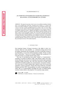
Fig. 1. Meandermigration along the Ram River, NWT, Canada, is constrained at some sites by resistant lithology(right center), but cutbank erosion is enhanced where glaciofluvialsedimentsare encountered (left).

S.J. Walsh et aL / Georaorphology 21 (1998) 183-205

type, and has consequences for conservation of biodiversity (Shankman, 1991). A channel may be abandoned by meander cutoff or chute development (Leopold et al., 1964). Each of these landforms is characterized by distinct alluvial deposits and in turn influences future sedimentation. Variation in sediment characteristics, particularly texture and chemical constituents may promote establishment and growth of some species at the expense of others. The importance of being able to distinguish the scale and origin of influence in riparian environments has been argued by Rostan et al. (1987), Baker (1989), Chauvet and Decamps (1989), Malanson (1993), and Schwarz et al. (1996). At a coarser scale, the development of abandoned channels are controlled by the flow of water across the floodplain and proximity of a site to the channel, and vegetation on the floodplain (e.g. James, 1985; Bhowmik and Demissie, 1989). The pattern of change within the abandoned channels arises from the finer processes and patterns of deposition in the eddies and slow water of obstructions and is also constrained by coarser-scale processes and patterns. If the processes and patterns of abandoned channels, channel and point bars, and cutbanks are created by specifics of erosion and deposition, and constrained by floodplain geometry and river flows, then these latter processes and patterns can be seen as created by the processes and patterns of channels, point bars, and cutbanks and constrained by coarserscale processes and patterns. The processes and patterns that are considered at this scale are those of floodplain dynamics. Floodplain dynamics, including meander dynamics, while arising from the processes of channel migration, are constrained by coarser-scale features such as valley width and geology (Fig. 1), and human activity in the drainage basin. One interesting feature of these constraints is that they can embody disequilibrium relations of processes and patterns. Paraglacial (sensu Church and Ryder, 1972) environments are a good example. In the Rocky Mountains of the USA and Canada, Quaternary glaciation created large loads of glacio-fluvial sediments that are stored in large terraces in mountain valleys. These features influence ongoing development of floodplain features in the valleys such as bars, cutbanks, and abandoned channels, by determining the sediment available during large floods as

195

Fig. 2. Spatial- and temporal-scaleissues are significantalong the Middle Fork of the Flathead River, northwest Montana, USA (foreground).A tributarystreamdischargesmodemsedimentsinto the river, and encounterscoarse-grainedrelict sedimentsdeposited in the valleyof the Middle Fork during Pleistocenedeglaciation. The modem Middle Fork is in disequilibrium with the massive quantities of paraglacial sediments.

well as overall valley geometry. Paraglacial sediments continue to enter the fluvial system through mass wasting because paraglacial terraces are eroded at cutbanks. The net result is that modem processes are in disequilibrium with the size and amount of sediments available for movement (Fig. 2), making any prediction of directional development of landforms problematic (Malanson and Butler, 1990, 1991). In a less obvious way, valleys in the midwest USA were created by glacial meltwaters at discharges much greater than experienced at present (Salisbury et al., 1968). As a result, the valley widths are large relative to ongoing processes. But valley widths created by processes in the past still constrain

196

S.J. Walsh et al. / Geomorphology 21 (1998) 183-205

current processes and patterns. Rex and Malanson (1990) found that valley width affected the shape of forest patches on modem floodplains. In the same area, the diversity of riparian wetlands is also affected by valley width, and particular events such as a major channel change of the Mississippi River can constrain local floodplain dynamics for ~ 100,000 years.

4.1. RS and GIS: analyzing the fluvial environment Techniques for analysis of scale, pattern, and process in the fluvial environment run the gamut from traditional mapping of changes in channel positions from aerial photographs (e.g. Brook and Luft, 1987; Whitesell et al., 1988; Marston et al., 1995; and references therein) to the use of sophisticated RS-GIS techniques. In some cases, the end result of a map of channel change developed using traditional aerial photography interpretation and ground truthing may be no different than a similar map developed via RS-GIS techniques. The latter has the advantage, however, of being more easily updated and quantifiable, and can be combined with DEM data to enhance the interpretation and the examination of related processes; for example, the work of Townsend et al. (1995), who used sequential Landsat TM images to illustrate an absence of channel change in the fluvial environment of the Roanoke River of eastern North Carolina over a 10-year period. With digitized maps of channel position resident within a GIS environment, it is feasible to map responses of landforms and riparian vegetation to possible flow alterations. Johnson et al. (1995) used flow data from the U.S. Geological Survey in concert with GIS mapping of landforms and vegetation based on aerial photographs to simulate effects of flow reduction on riparian vegetation of the Snake River, Idaho. On-going research examining the Roanoke River floodplain of North Carolina is also identifying relationships between discharge fluctuations resulting from dam releases and corresponding riparian responses (Walsh and Townsend, 1995). Issues of spatial heterogeneity of geomorphic/vegetation interactions have recently been examined by Mertes et al. (1995) and Townsend and Butler (1996). In the former study, the spatial heterogeneity of hydrology and vegetation during high-water periods in geomorphologically distinct

reaches of the Amazon River was determined using semivariance statistics. Those statistics were derived from data extracted from three classified Landsat TM images covering the upper, middle, and lower portions of the drainage basin. The highest diversity of vegetation types occurred along floodplain drainage channels, and the middle reach of the river had the highest diversity of wetland classes. Floodplain landforms available for colonization were mapped by interpreting the Landsat imagery. Townsend et al. (1995) and Walsh and Townsend (1995) interpreted and ground-truthed 1984 and 1993 Landsat TM imagery in concert with an integrated GIS to map landform types along the lower floodplain of the Roanoke River, North Carolina, and identified and quantified the area of vegetation classes associated with specific landform types. Included in their analyses was a landuse/vegetation category identified as beaver (Castor canadensis) ponds. In a follow-up study, Townsend and Butler (1996) used the same imagery and interpreted maps to illustrate a tenfold increase in the area occupied by beaver on the floodplain. The GIS determined transitions in the landcover classification, calculated edge metrics for the beaver ponds, and determined adjacency of ponds. The increase in beaver activity over the time covered by the images increased the length of beaver-pond edges and associated habitat on the floodplain, and decreased the isolation of individual beaver ponds (as measured using the mean nearest-neighbor distance option resident within the FRAGSTATS package). Distance between the nearest-neighbor beaverpond patch decreased from 415 to 93 m. The direct observation of riparian vegetation has been historically difficult because of the interference of the forest canopy. Yamagata and Akiyama (1988), Muller et al. (1993), and Schultz (1993) have reported some success in using Landsat TM data to map areas of surface flooding and soil moisture variation in forested floodplains. Satellite-based synthetic aperture radar data have recently emerged as a potentially useful system to map sub-canopy characteristics in riparian and floodplain environments (Place, 1985; Ormsby and Blanchard, 1985; Hess et al., 1990; Sippel et al., 1994; Wang et al., 1995) and soil moisture variations beneath forest canopies (Engroan, 1990; Beaudoin et al., 1990; Pietroniro et al., 1993).

S.J. Walsh et al. / Geomorphology 21 (1998) 183-205

5. Case study: the alpine environment Examples of scale dependence in both spatial and temporal contexts abound in the alpine environment. Temporal-scale dependence is illustrated, for exam-

197

pie, in the influences of the Pleistocene Ice Age and subsequent paraglacial sedimentation whose effects are still important in alpine fluvial systems. Influences of earlier periods extend, however, beyond the fluvial environment. Butler and Malanson (1990)

Fig. 3. Debris flows illustrating similar morphologies transcending spatial scales. (a) A debris flow in glacial till. Note the foot at lower left for scale. (b) Intermediate-scale debris flows resulting from heavy rain and rapid snowmelt. (e) Sturzstrom deposits impounding two lakes along the base of the Lewis Overthrust Fault (at base of cliff on right). Sturzstrom lobes ca. 1-km long. (d) Person for scale, standing in center of lower sturzstrom lobe impounding the smaller lake in (c).

198

S.J. Walsh et al. / Geomorphology 21 (1998) 183-205

illustrated that current rates of geomorphic processes could not explain the depth of incision of subalpine snow-avalanche paths in southern Glacier National Park (GNP), Montana, and concluded that dramatically greater rates characterized the Late Pleistocene/early Holocene. Temporal-scale issues are also revealed in more recent time spans. The Little Ice Age produced the most extensive glacial advance in the northern Rockies of Montana and Alberta since the Pleistocene (Carrara, 1987; Buffer, 1989b). The effects of this period of glacial advance are still evident on the landscape in on-going succession of vegetation, unstable morainal slopes prone to mass movement, and glacial lakes behind Little Ice Age terminal moraines. Mass movements in GNP provide an interesting example of landform morphologies that extend along the scale continuum (Buffer, 1983). Debris flows occur at scales ranging from micro-scale flows a few centimeters in width and several meters in length (Fig. 3a), through intermediate-scale features such as mapped and described by Butler and Walsh (1994), and Butler and Malanson (1996) (Fig. 3b), to massive sturzstroms that have left behind deposits sufficient to impound kilometer-long lakes (Fig. 3c) (Butler et al., 1986; Butler and Malanson, 1993a). Each scale of flow deposit possesses virtually identical flow morphology typified by transverse and longitudinal ridges and furrows, such that it becomes impossible to discern the size of a deposit when viewed in a photograph unless some scale indicator is provided (Fig. 3d). The scale relations of process and pattern are also seen for mass movements. Individual flows are the processes that create the abrupt topography of the eastern front of the Rocky Mountains in GNP, but these flows are linked to the coarse-scale landscape features of the Lewis Overthrust Fault (LOF), along which the mass movements occur (Fig. 3c). At the LOF resistant Precambrian limestones and argillites overlie weak Cretaceous mudstones. An assortment of mass movement features occur along the entire exposed length of the fault. Thus the pattern of mass movement in this region is produced by the processes of landslide, slump, and sturzstroms, but is constrained by the position of the LOF, the rate of exposure of which is determined by the mass movements that are the slope-retreat processes here.

Fig. 4. The influences of scale in the alpine environment are illustrated where finer-scale processes and patterns are limited in their areal extent to the surface of coarser-scale landforms and more widespread processes. Without the concentration of finergrained sediments along the front and on the surface of the solifluction treads, frost-churningwould be unlikely to accomplish the finer-scaled development of patterned ground that characterizes such sites.

In the alpine tundra of GNP, the development of periglacial patterned ground illustrates the principle of scale dependence. There, miniature patterned ground has developed on the treads of solifluction terraces (Fig. 4) (Buffer and Malanson, 1989). Without the presence of the finer-grained solifluction treads, it is doubtful if the current patterned ground would have developed. The finer-scaled pattern is, therefore, dependent on the coarser-scaled spatial pattern, and also influenced by the temporal dimension. Scale dependence is also illustrated in patterns and controls of alpine treeline in GNP. The position of alpine treeline in GNP is a result of a complex

S.J. Walsh et al. /Geomorphology 21 (1998) 183-205

interaction of topographic, geomorphic, climatic, and vegetation factors (Walsh et al., 1989, 1992, 1994a,b; Walsh, 1993; Butler and Walsh, 1994; Malanson and Butler, 1994), operating at scales ranging from the landscape (ca. 100-10,000 ha) down to individual treeline stands (0.1--1 ha) and even to individual plants ( < 0.1 ha) (Brown et al., 1994; Cairns, 1994). 5.1. RS and GIS: analyzing the alpine environment

Because temporal- and spatial-scale issues are inherent in alpine environments, recognition and incorporation into a hierarchical geographic information system is vital. Walker et al. (1993) have developed such a system for their studies of the relationships among vegetation, wind, snow, topography, and temperature regiimes at the Niwot Ridge LongTerm Ecological Research Site in Colorado, USA. Our own research, :and that of our associates, has generally been organized around four primary methodological initi~ttives: 1. development of a GIS to support spatial and biophysical studies of processes and feature distributions (including distribution of alpine treeline, snow-avalanche paths, debris flows, snow patches, and wet and dry aJpine tundra sites) (Walsh et al., 1989, 1992, 1994a,b; Walsh, 1993; Allen and Walsh, 1996); 2. implementation of resource evaluation studies through the manipulation of the derived GIS database, for the evaluation of natural hazards from landslides, debris flows, and snow avalanches; assessment of lake turbidity levels and relationships with basin morphometry; identification of deltaic wetlands; and evaluation of forest fire potential (Butler and Walsh, 1990, 1994; Walsh et al., 1990a,b; Butler et al., 1991a,b,c; Brown and Walsh, 1991, 1992); 3. examination of scale dependencies of plant biomass and topography, and spatial analyses of derived pattems of the distributions of specific phenomena (Bian and Walsh, 1993; Brown et al., 1994; Allen and Walsh, 1996; Walsh et al., 1997b); 4. cartographic and quantitative modelling of disturbance factors and topoclimatic variables affecting the biophysical landscape at the alpine treeline ecotone (Walsh e~I al., 1990a,b; Walsh and Kelly,

199

1990; Malanson and Cairns, 1995; Allen and Walsh, 1996). Through those initiatives, Allen and Walsh (1993) used interseasonal Landsat MSS digital data to characterize snow accumulation and ablation patterns in GNP through a satellite time-series. The satellite data were classified according to a priori snow classes, i.e. full snowcover, partial snowcover, and snow-free. Markov transition probabilities were used to examine the change in state of the snowcover conditions over time and space for the study area as a whole. A DEM was used to stratify the study area according to elevation, slope aspect, and slope angle zones. Transition probabilities were applied to each zone to assess the change (from and to) of snow conditions for specific topographic settings. Elevation, slope angle, and slope aspect variables are often used to assess the local orientation of the landscape. Such measures are subsequently used to derive slope convexity/concavity conditions and resource potential surfaces. Topographic curvature integrates planform and profile curvature to portray localized topographic situation (Moore et al., 1991). The variable distinguishes slopes having a convex versus a concave slope. Profile curvature is the vertical or downslope concavity/convexity and portrays slope steepness. Slope curvature affects the acceleration and deceleration of gravity flows. Solar radiation affects the soil moisture, temperature regimes, and photosynthetic capacity of the landscape. The potential direct solar insolation at any location can be represented through grid locations throughout the study area, given DEM-derived elevation, slope angle, and slope aspect information. The procedures are modeled after Bonan (1989) and Montieth and Unsworth (1990). Shadowing by adjacent terrain is an important factor influencing potential insolation. An algorithm for evaluating whether a cell is in shadow at any given time is included in our solar estimation algorithms. The resulting GIS layer represents the relative potential for solar radiation at every pixel throughout the growing season. Solar radiation potential is derived by integrating the effects of shadows, direct solar insolation, and insolation variability throughout the normal growing season within the study area. Values can be calculated for various time steps on an hourly, daily, or seasonal basis.

200

s.J. Walsh et al. / Geomorphology 21 (1998) 183-205

A common approach to simulating soil moisture is to apply an index based on the log of the accumulation of flow from upslope cells in a DEM divided by the surface slope angle (Beven, 1978). Soil moisture potential can be estimated using an index of saturation potential developed by Beven and Kirkby (1979), and calculated by using flow directions and accumulation grids based on eight directions for pixel-to-pixel flow routing after Moore et al. (1991). Topographic wetness potential provides a simple but effective model that characterizes channels, gullies, and moisture sinks (Allen and Walsh, 1996). The programs used to calculate the index (Wolock, 1988) have been adapted to accept raster data represented as DEMs and to output a raster GIS file representing the relative potential for soil saturation (Brown, 1991, 1992). Townsend and Walsh (1996) used such an approach to derive and compare the potential values of soil moisture generated through a variety of terrain and soil measurement approaches. A digitized hydrography layer was used to support the calculation of the index. A measure of landscape accessibility to hydrographic features can also be computed to assess moisture availability by defining the mean distance of each pixel of a selected landscape partition (e.g. watershed, avalanche path run-out zone, or cirque area) to the nearest hydrographic feature (Walsh et al., 1997b). Exposure and shelteredness also affect a variety of biophysical gradients and disturbances at alpine treeline (Allen, 1995). The McNab (1993) landform index quantifies the effects of mesoscale landforms on site productivity. The index uses the vertical gradient to the topographic horizon in its calculation. The index is highly correlated with slope position. Lapen and Martz (1993) have developed fetch and directional relief indices to quantify wind sheltering. The directional relief uses a DEM to quantify the relative height of a target cell to its neighborhood as a surrogate for exposure or shelteredness. Allen (1995) used the indices to examine alpine treeline in the GNP. He specified a southwest wind direction and a 3.0 km search window from target cells in the calculation of the indices. A DEM was used by Allen (1995) and Allen and Walsh (1996) to stratify the alpine landscape on the basis of hillslope homogeneity through the recursive subdivision of the landscape into stream channels and ridges. A slope strati-

fication algorithm was applied to segment the study area into basins and corresponding sub-basins that had low topographic variances (Band, 1989). Scaling relationships exist across a range of spatial scales, and the strength, direction, and type of relationship also vary across scale. Bian and Walsh (1993) explored the scale dependence in GNP between elevation, slope angle, and slope aspect, derived from GIS-based DEMs, and plant biomass, defined through satellite digital data. They sought to address: (a) the effective range of spatial scales within which plant biomass and terrain variables were spatially dependent; (b) optimum spatial scales for representing terrain and plant relationships; and (c) the degree of spatial dependence of these relationships. Scale-dependent relationships between topography and vegetation were related to the glacial history of the study area, particularly the spatial organization and dimensionality of the U-shaped ridge-valley system. Brown (1991) showed the importance of watershed-level versus regional-scale models for estimating the nature of the alpine treeline ecotone in GNP. Disturbance, principally snowavalanche paths and debris flows, were shown to be locally important factors in explaining the composition of the alpine treeline ecotone (Butler and Walsh, 1994). Walsh et al. (1997a,b) examined the relationship between vegetation and terrain by deriving satellitebased NDVI measures: a landcover classification (e.g. snow and ice, barren, meadow/tundra, shrub/krummholz, open canopy forest, and closed canopy forest), GIS-based terrain variables (elevation, slope angle, slope aspect, and solar radiation), pattern variables (mean, variance, coefficient of variation, Moran's index of spatial autocorrelation, and fractal dimension), and a series of linear regression models in order to test the relationships between vegetation and terrain characteristics in GNP extending from 30 X 30 m through nine resolution steps culminating at 1050 x 1050 m. Their findings suggest: 1. an increased explanation of NDVI at moderate and coarse scales; 2. importance of local-scale topographic orientation on plant productivity evidence by the inclusion of slope angle and solar radiation potential in the regression equations;

S.J. Walsh et aL / Geomorphology 21 (1998) 183-205

3. increased slope aagle associated with a decrease in NDVI values (snow-avalanche paths and debris flows are common disturbances in areas of steep slopes, whereas topographic benches and sheltered areas can support highly productive alpine meadows and meadow/krummholz vegetation); 4. spatial autocorrelation of NDVI, at coarser scales, increased, and elevation emerged as the dominant descriptor variable in the regression models because of the pronounced topographic gradient within GNP and dae local nature of the geomorphic disturbance regime; 5. spatial organization of NDVI at finer scales is an important descriptor variable of NDVI at coarser spatial scales; 6. terrain orientation variables and elevation were important for characterizing the variation in NDVI when controlled fix the type of landcover.

6. Conclusions Geomorphology has traditionally been a discipline with roots sunk firrrdy in the remote sensing field through measurement and interpretation of aerial photography. We see no reason why this tradition will not continue. The modern technologies of remote sensing and GIS will not detract from this rich heritage. Instead, these efficient tools allow geomorphologists to examine spatial relationships at a variety of scales that would not be feasible using only fieldwork or traditional aerial photography. Temporal changes can also be examined effectively as sequential images provide insights into process and pattern. And yet, as we stated early in this paper, the spatial limitations of satellite imagery and the corresponding GIS environments in which such images reside and are analyzed provide ample opportunities for, and indeed requiie that, fieldwork will always be an integral part of the discipline. The advent of the quantitative revolution and the development of sophisticated models advance and expand the horizons of the science of geomorphology. The capabilities of remote sensing and geographic information systems will allow such advances and expansions to continue in a partnership with the traditions of the discipline.

201

References Allen, T.R., 1995. Relationships between Spatial Pattern and Environment at The Alpine Treeline Ecotone, Glacier National Park, Montana. Unpubl. Doct. Diss., Dep. of Geography, Univ. of North Carolina, Chapel Hill. Allen, T.R., Walsh, S.J., 1993, Characterizing multitemporal alpine snowmelt patterns for ecological inferences. Photogramm. Eng. Remote Sensing 59 (10), 1521-1529. Allen, T.R., Walsh, S.J., 1996. Spatial and compositional pattern of Alpine Treeline, Glacier National Park, Montana. Photogramm. Eng. Remote Sensing 62 (11), 1261-1268. Arno, S.F., Reinhardt, E.D., Scott, J.H., 1993. Forest structure and landscape patterns in the subalpine lodgepole pine type: a procedure for quantifying past and present conditions. USDA Forest Service, Intermountaln Research Station, Gen. Tech. Rep. 1NT-294, 17 pp. Aronoff, S., 1989. Geographic Information Systems: A Management Perspective. WDL Publications, Ottawa. Baker, W.L., 1989. Macro- and micro-scale influences on riparian vegetation in western Colorado. Ann. Assoc. Am. Geogr. 79, 65-78. Baker, W.L., Cai, Y., 1992. The r.le programs for multiscale analysis of landscape structure using the GRASS geographical information system. Landscape Ecol. 7 (4), 291-302. Band, L.E., 1989. Spatial aggregation of complex terrain. Geogr. Anal. 21,279-293. Beaudoin, A., Le Toan, T., Gwyn, Q.H.W., 1990. SAR observations and modelling of the C-Band backscatter variability due to multiscale geometry and soil moisture. IEEE Trans. Geosci. Remote Sensing 28 (5), 886-895. Bendix, J., 1994. Scale, direction, and pattern in riparian vegetation-environment relationships. Ann. Assoc. Am. Geogr. 84 (4), 652-665. Beven, K.J., 1978. The hydrological response of headwater and sideslope areas. Hydrol. Sci. Bull. 23 (4), 419-437. Beven, K.J., Kirkby, M.J., 1979. A physically-based variable contributing area model of basin hydrology. Hydrol. Sci. Bull. 24 (1), 43-69. Bhowmik, N.G., Demissie, M., 1989. Sedimentation on the Illinois River valley and backwater lakes. J. Hydrol. 105, 187195. Bian, L., Walsh, S.J., 1993. Scale dependencies of vegetation and topography in a mountainous environment of Montana. Prof. Geogr. 45 (1), 1-11. Bishop, M.P., Shroder, J.F. Jr., Ward, J.L., 1995. SPOT multispectral analysis for producing supraglacial debris-load estimates for Batura Glacier, Pakistan. GeoCarto Int. l0 (4), 81-90.

Bonan, G.B., 1989. A computer model of the solar radiation, soil moisture, and soil thermal regimes in boreal forests. Ecol. ModeU. 45, 275-306. Brook, G.A., Luft, E.R., 1987. Channel pattern changes along the lower Oconee River, Georgia, 1805/7 to 1949. Phys. Geogr. 8 (3), 191-209. Brown, D.G., 1991. Topoclimatic models of an alpine environ-

202

S.J. Walsh et al. / Geomorphology 21 (1998) 183-205

ment using digital elevation models within a GIS. Proc. GIS/LIS Conf. 1, Atlanta, GA, pp. 835-844. Brown, D.G., 1992. Topographical and biophysical modelling of vegetation patterns at alpine treeline. Doct. Diss., Univ. of North Carolina, Dep. of Geography, Chapel Hill, 238 pp. Brown, D.G., Walsh, S.J., 1991. Compatibility of non-synchronous in-situ water quality data and remotely-sensed spectral information for assessing lake turbidity levels in complex and inaccessible terrain. Geocarto Int. 4 (2), 5-11. Brown, D.G., Walsh, S.J., 1992. Relationships between the morphometry of alpine and subalpine basins and remotely-sensed estimates of lake turbidity, Glacier National Park, Montana. Phys. Geogr. 13 (3), 250-272. Brown, D.G., Bian, L., Walsh, S.J., 1993. Response of a distributed watershed erosion model to variations in input data aggregation levels. Comput. Geosci. 19 (4), 499-509. Brown, D.G., Cairns, D.M., Malanson, G.P., Walsh, S.J., Butler, D.R., 1994. Remote sensing and GIS techniques for spatial and biophysical analyses of alpine treeline through process and empirical models. In: Michener, W.K., Brunt, J.W., Stafford, S.G. (Eds.), Environmental Information Management and Analysis: Ecosystem to Global Scales. Taylor and Francis, London, pp. 453-481. Butler, D.R., 1983. Rockfall hazard inventory, Ram River, Mackenzie Mountains. Can. Geogr. 27 (2), 175-178. Butler, D.R., 1989a. The failure of beaver dams and resulting outburst flooding: a geomorphic hazard of the southeastern Piedmont. Geogr. Bull. 31 (1), 29-38. Butler, D.R., 1989b. Glacial hazards in Glacier National Park, Montana. Phys. Geogr. 10 (1), 53-71. Butler, D.R., Malanson, G.P., 1989. Periglacial patterned ground, Waterton-Glacier International Peace Park, Canada and U.S.A. Z. Geomorphol. 33 (1), 43-57. Butler, D.R., Malanson, G.P., 1990. Non-equilibrium geomorphic processes and patterns on avalanche paths in the northern Rocky Mountains, U.S.A.Z. Geomorphol. 34 (3), 257-270. Butler, D.R., Malanson, G.P., 1993a. Characteristics of two landslide-dammed lakes in a glaciated alpine environment. Limnol. Oceanogr. 38 (2), 441-445. Buffer, D.R., Malanson, G.P., 1993b. An unusual early-winter flood and its varying geomorphic impact along a subalpine river in the Rocky Mountains of Montana, USA. Z. Geomorphol. 37, 145-155. Butler, D.R., Malanson, G.P., 1996. A major sediment pulse in a subalpine river caused by debris flows. Z. Geomorphol. 40 (4), 525-535. Butler, D.R., Walsh, S.J., 1990. Lithologic, structural, and topographic influences on snow-avalanche path location, eastern Glacier National Park, Montana. Ann. Assoc. Am. Geogr. 80 (3), 362-378. Butler, D.R., Walsh, S.J., 1994. Site characteristics of debris flows and their relationship to alpine treeline. Phys. Geogr. 15 (2), 166-180. Buffer, D.R., Oelfke, J.G., Oelfke, L.A., 1986. Historic rockfall avalanches, northeastern Glacier National Park, Montana, U.S.A. Mt. Res. Dev. 6 (3), 261-271. Butler, D.R., Malanson, G.P., Walsh, S.J., 1991a. Identification of

deltaic wetlands at montane finger lakes, Montana. Environ. Prof. 13, 352-362. Butler, D.R., Walsh, S.J., Brown, D.G., 1991b. Three-dimensional displays for natural hazards analysis, using classified Landsat Thematic Mapper digital data and large-scale digital elevation models. GeoCarto Int. 4, 65-69. Buffer, D.R., Walsh, S.J., Malanson, G.P., 1991c. GIS applications to the indirect effects of forest fires in mountainous terrain. In: Nodvin, S.C., Waldrop, T.A. (Eds.), Fire and the Environment: Ecological and Cultural Perspectives. U.S. Department of Agriculture, Southeast Forest Experiment Station, Asheville, NC, pp. 202-211. Cairns, D.M., 1994. Development of a physiologically mechanistic model for use at the alpine treeline ecotone. Phys. Geogr. 15 (2), 104-124. Carrara, P.E., 1987. Holocene and latest Pleistocene glacial chronology, Glacier National Park, Montana. Can. J. Earth Sci. 24, 387-395. Chauvet, E., Decamps, H., 1989. Lateral interactions in a fluvial landscape: the River Garonne, France. J. N. Am. Benthol. Soc. 8, 9-17. Chrisman, N., 1997. Exploring Geographic Information Systems. John Wiley, New York. Church, M., Ryder, J.M., 1972. Paraglacial sedimentation: a consideration of fluvial processes conditioned by glaciation. Bull. Geol. Soc. Am. 83, 3059-3072. Cihlar, J., Pultz, T.J., Gray, A.L., 1992. Change detection with synthetic aperture radar. Int. J. Remote Sensing 13 (3), 401414. Civco, D.L., 1989. Topographic normalization of Landsat Thematic Mapper digital imagery. Photogramm. Eng. Remote Sensing 55(9), 1303-1310. Clifford, N.J., Richards, K.S., Brown, R.A., Lane, S.N., 1995. Scales of variation of suspended sediment concentration and turbidity in a glacial meltwater stream. Geogr. Ann. 77A, 45-65. Colby, J.D., 1991. Topographic normalization in ruged terrain. Photogramm. Eng. Remote Sensing 57(5), 531-537. Congalton, R.G., 1991. A review of assessing the accuracy of classification of remotely sensed data. Remote Sensing Environ. 37, 35-46. Congalton, R.G., Mead, R.A., 1983. A quantitative method to test for consistency and correctness in photointerpretation. Photogramm. Eng. Remote Sensing 49, 67-74. DeCola, L., 1989. Fractal analysis of a classified Landsat scene. Photogramm. Eng. Remote Sensing 55 (5), 601-610. DeCola, L., Montagne, N., 1993. The PYRAMID system for multiscale raster analysis. Comput. Geosci. 19 (10), 13931404. DeGraff, J.V., Romesburg, H.C., 1980. Regional landslide-susceptibility assessment for wildland management: a matrix approach. In: Coates, D.R., Vitek, J.D. (Eds.), Tresholds in Geomorphology. George Allen & Unwin, London, pp. 401414. Dikau, R., Cavallin, A., J~iger, S., 1996. Databases and GIS for landslide research in Europe. Geomorphology 15 (3-4), 227239.

S.J. Walsh et al. / Geomorphology 21 (1998) 183-205 Engman, E.T., 1990. Progress in microwave remote sensing of soil moisture. Can. J. }Remote Sensing 16 (3), 6-14. Forman, R.T.T., Godron, lvl., 1981. Patches and structural components for a landscape ecology. BioScience 31,733-740. Forman, R.T.T., Godron, M., 1986. Landscape Ecology. John Wiley, New York, 619 pp. Franklin, S.E., 1990. Topographic context of satellite spectral response. Comput. Geosci. 16, 1003-1010. Gamble, D.W., Meentemeyer, V., 1996. The role of scale in research on the Himalaya-Ganges-Brahmaputra interaction. Mt. Res. Dev. 16 (2), 149-155. Gao, J., Lo, C.P., 1995. Micro-scale modelling of terrain susceptibility to landsliding from a DEM: a GIS approach. Geocarto Int. 10 (4), 15-30. Gao, J., Xia, Z.-g., 1996. Fractals in physical geography. Prog. Phys. Geogr. 20 (2), 178-191. Gosz, J.R., 1993. Ecotone hierarchies. Ecol. Appl. 3 (3), 369-373. Gruber, U., Haefner, H., 1995. Avalanche hazard mapping with satellite data and a digital elevation model. Appl. Geogr. 15 (2), 99-113. Gupta, R.P., Joshi, B., 1990. Landslide hazard zoning using the GIS approach - - a case study from the Ramganga Catchment, Himalayas. Eng. Geol. 28, 119-131. Harden, C.P., 1993. Upland erosion and sediment yield in a large Andean drainage basin. Phys. Geogr. 14 (3), 254-271. Hess, L.L., Melack, J.M., Siminett, D.S., 1990. Radar detection of flooding beneath the forest canopy: a review. Int. J. Remote Sensing 11 (7), 1313-11325. Hudson, W.D., Ramm, CW., 1987. Correct formulation of the Kappa coefficient of agreement. Photogramm. Eng. Remote Sensing 53 (4), 421-422. Hunsaker, C.T., Levine, D.A., 1995. Hierarchical approaches to the study of water quality in rivers. Bioscience 45 (3), 193203. Imhoff, M.L., Gesch, D.B., 1990. The derivation of a sub-canopy digital terrain model of a flooded forest using synthetic aperture radar. Photogramm. Eng. Remote Sensing 56 (8), 11551162. James, C.S., 1985. Sediment transfer to overbank sections. J. Hydraul. Res. 27 (5), 435-452. Jensen, J.R., 1996. Intloductory Digital Image Processing: A Remote Sensing Perspective. Prentice-Hall, Englewood Cliffs, NJ, 379 pp. Joao, E.M., Walsh, S.J., 1'992. Interfacing GIS to a hydrological model: simulation of non-point pollution generated by the location of urban development. Comput., Environ., Urban Syst. 16, 43-63. Johnson, W.C., Dixon, M.D., Simons, R., Jenson, S., Larson, K., 1995. Mapping the response of riparian vegetation to possible flow reductions in the Snake River, Idaho. Geomorphology 13, 159-173. Johnston, C.A., Naiman, RJ., 1990. The use of a geographic information system to analyze long-term landscape alteration by beaver. Landscape Ecol. 4 (1), 5-19. Kasischke, E.S., Bourgeau-Chavez, L.L., Christensen, N.L., Haney, E., 1994. Observations on the sensitivity of ERS-1 SAR image intensity to changes in aboveground biomass in

203

young loblolly pine forests. Int. J. Remote Sensing 15 (1), 3-16. Langran, G., 1992. Time in Geographic Information Systems. Taylor and Francis, London. Lapen, D.R., Martz, L.W., 1993. The measurement of two simple topographic indices of wind sheltering/exposure from raster digital elevation models. Comput. Geosci. 19 (6), 769-779. Leopold, L.B., Wolman, M.G., Miller, J.P., 1964. Fluvial Processes in Geomorphology. W.H. Freeman, San Francisco, CA. Lillesand, T.M., Kiefer, R.W., 1994. Remote Sensing and Image Interpretation. John Wiley, New York. Malanson, G.P., 1993. Riparian Landscapes. Cambridge University Press, Cambridge. Malanson, G.P., Butler, D.R., 1990. Woody debris, sediment and riparian vegetation of a subalpine river, Montana, U.S.A. Arct. Alp. Res. 22 (2), 183-194. Malanson, G.P., Butler, D.R., 1991. Floristic variation among gravel bars in a subalpine river. Arct. Alp. Res. 23 (3), 273-278. Malanson, G.P., Butler, D.R., 1994. Tree-tundra competitive hierarchies, soil fertility gradients, and treeline elevation in Glacier National Park, Montana. Phys. Geogr. 15 (2), 166-180. Malanson, G.P., Cairns, D.M., 1995. Effects of increased cloudcover on a montane forest landscape. Ecoscience 2 (1), 75-82. Marston, R.A., Girel, J., Pautou, G., Piegay, H., Bravard, J.-P., Ameson, C., 1995. Channel metamorphosis, floodplain disturbance, and vegetation development: Ain River, France. Geomorphology 13, 121-131. McDonnell, R.A., 1996. Including the spatial dimension: using geographic information systems in hydrology. Prog. Phys. Geogr. 20 (2), 159-177. McGarigal, K., Marks, B.J., 1993. FRAGSTATS: Spatial Pattern Analysis for Quantifying Landscape, Version 1.0. Forest Science Department, Oregon State University, Corvallis, OR. McNab, W.H., 1993. A topographic index to quantify the effect of mesoscale landform on site productivity. Can. J. For. Res. 23, 1100-1107.

Meentemeyer, R.K., Butler, D.R., 1995. Temporal and spatial changes in beaver pond locations, eastern Glacier National Park, Montana, USA. Geogr. Bull. 37 (2), 97-104. Meentemeyer, V., 1989. Geographical perspectives of space, time, and scale. Landscape Ecol. 3 (3/4), 163-173. Meentemeyer, V., Box, E.O., 1987. Scale effects in landscape studies. In: Turner, M.G. (Ed.), Landscape Heterogeneity and Disturbance. Ecological Studies, 64, Springer-Verlag, New York, pp. 15-34. Mejia-Navarro, M., Wohl, E.E., Oaks, S.D., 1994. Geological hazards, vulnerability, and risk assessment using GIS: model for Glenwood Springs, Colorado. Geomorphology 10 (1-4), 331-354. Merot, P., Crave, A., Gascuel-Odoux, C., Louhala, S., 1994. Effect of saturated area on backscattering coefficient of the ERS 1 synthetic aperture radar: First results. Water Resour. Res, 30 (2), 175-179. Mertes, L.A.K., Daniel, D.L., Melack, J.M., Nelson, B., Martinelli, L.A., Forsberg, B.R., 1995. Spatial patterns of hydrology, geomorphology, and vegetation on the floodplain of the

204

S.J. Walsh et al. / Geomorphology 21 (1998) 183-205

Amazon River in Brazil from a remote sensing perspective. Geomorphology 13, 215-232. Meyer, P., Itten, K.I., Kellenberger, T., Sandmeier, S., Sandmeier, R., 1993. Radiometric corrections of topographically induced effects on Landsat TM data in an alpine environment. Int. Soc. Photogramm. Remote Sensing, J. Photogramm. Remote Sensing 48 (4), 17-28. Milne, B.T., 1990. Lessons from applying fractal models to landscape patterns. In: Turner, M.G., Gardner, R.H. (Eds.), Quantitative Method in Landscape Ecology. Springer-Verlag, New York, pp. 199-235. Montieth, J.L., Unsworth, M.H., 1990. Principals of Environmental Physics. Edward Arnold, London. Moore, I.D., Grayson, R.B., Landson, A.R., 1991. Digital terrain modelling: a review of hydrological, geomorphological, and biological applications. Hydrol. Process. 5, 3-30. Muller, E., Decamps, H., Dobson, M.K., 1993. Contribution of space remote sensing to river studies. Freshwater Biol. 29, 301-312. Nellis, M.D., Briggs, J.M., 1989. The effect of spatial scale on Konza landscape classification using textural analysis. Landscape Ecol. 2 (2), 93-100. Nemani, R., Pierce, L., Running, S., Band, L., 1993. Forest ecosystem processes at the watershed scale: sensitivity to remotely-sensed leaf area index estimates. Int. J. Remote Sensing 14, 2519-2526. O'Neill, R.V., Krummel, J.T., Gardner, R.H., Sugihara, G., Jackson, B., DeAngelis, D.L., Milne, B.T., Turner, M.G., Zygmunt, B., Cbxistensen, S.W., Dale, V.H., Graham, R.L., 1988. Indices of landscape pattern. Landscape Ecol. 1 (3), 153-162. Ormsby, J.B., Blanchard, B.J., 1985. Detection of lowland flooding using active microwave systems. Photogramm. Eng. Remote Sensing 51 (3), 317-328. Parker, K.C., Bendix, J., 1996. Landscape-scale geomorphic influences on vegetation patterns in four environments. Phys. Geogr. 17 (2), 113-141. Pastor, J., Broschart, M., 1990. The spatial pattern of a northern conifer-hardwood landscape. Landscape Ecol. 4 (1), 55-68. Phillips, J.D., 1988. The role of spatial scale in geomorphic systems. Geogr. Anal. 20, 359-368. Phillips, J.D., 1995. Biogeomorphology and landscape evolution: the problem of scale. Geomorphology 13, 337-347. Pietroniro, A., Soulis, E.D., Kouwen, N., Rotunno, O., Mullins, D.W., 1993. Extracting distributed soil moisture information from C-band wide swath SAR imagery. Can. J. Remote Sensing 19 (1), 77-82. Place, J.L., 1985. Mapping of forested wetland: use of Seasat radar images to complement conventional sources. Prof. Geogr. 37 (4), 463-469. Plomick, R.E., Gardner, G.H., O'Neill, R.V., 1993. Lacunarity indices as measures of landscape texture. Landscape Ecol. 8 (3), 201-211. Price, M.F., Heywood, D.I. (Eds.), 1994. Mountain Environments and Geographic Information Systems. Taylor and Francis, London. Reineck, H.E., Singh, I.B., 1973. Depositional Sedimentary Environments. Springer-Verlag, New York.

Rex, K.D., Malanson, G.P., 1990. The fractal shape of riparian forest patches. Landscape Ecol. 4, 249-258. Ricketts, T.H., Birnie, R.W., Bryant, E.S., Kimball, K.D., 1993. Landsat TM mapping of alpine vegetation to monitor global climate change. Proc., 4th American Congress of Surveying and Mapping and the American Society for Photogrammetry and Remote Sensing, New Orleans, LA, pp. 86-97. Rignot, E.J., van Zyl, J.J., 1993. Change detection techniques for ERS-1 SAR data. IEEE Trans. Geosci. Remote Sensing 31 (4), 896-906. Risser, P.G., Karr, J.R., Forman, R.T.T., 1984. Landscape ecology: directions and approaches. Illinois Natural History Survey, Champaign, IL, Spec. Publ. 2, 18 pp. Robinove, C.J., 1982. Computation with physical values from Landsat digital data. Photogramm. Eng. Remote Sensing 48 (5), 781-784. Rogowkis, A.S., 1996. Quantifying soil variability in GIS applications, II. Spatial distribution of soil properties. Int. J. Geogr. Inf. Syst. 10 (4), 455-475. Romme, W.H., 1982. Fire and landscape diversity in subalpine forests of Yellowstone National Park. Ecol. Monogr. 52 (2), 199-221. Rostan, J.C., Amoros, C., Juget, J., 1987. The organic content of the surficial sediment: a method for the study of ecosystems development in abandoned river channels. Hydrobiologia 148, 45 -62. Salisbury, N.E., Knox, J.C., Stephenson, R.A., 1968. The valleys of Iowa 1: valley width and stream discharge relationships in the major streams. Iowa Studies in Geography No. 5, Univ. of Iowa, Iowa City, 107 pp. Schultz, G.A., 1993. Application of GIS and remote sensing in hydrology. In: Kovar, K., Nachtnebel, H.P. (Eds.), Application of Geographic Information Systems in Hydrology and Water Resources Management. IAHS Publ. 211, 127-140. Schwarz, W.L., Malanson, G.P., Weinrich, F., 1996. Effect of landscape position on the sediment chemistry of abandonedchannel wetlands. Landscape Ecol. 11, 27-38. Shankman, D., 1991. Channel migration and vegetation patterns in the southeastern coastal plain. Conservation Biol. 7, 176-183. Shankman, D., Drake, L.G., 1990. Channel migration and regeneration of bald cypress in western Tennessee. Phys. Geogr. 11, 343-352. Sippel, S.J., Hamilton, S.K., Melack, J.M., Choudhury, B.J., 1994. Determination of inundation area in the Amazon River floodplain using the SMMR 37 GHz polarization difference. Remote Sensing Environ. 48, 70-76. Townsend, P.A., Buffer, D.R., 1996. Patterns of landscape use by beaver on the lower Roanoke River floodplain, North Carolina. Phys. Geogr. 17 (3), 253-269. Townsend, P.A., Walsh, S.J., 1996. Spatial variability of a wetness model to soil parameter estimation approaches. Earth Surf. Process. Landf. 21,307-326. Townsend, P.A., Walsh, S.J., Buffer, D.R., 1995. Beaver pond identification through a satellite-based ecological habitat classification. Proc., American Society for Photogrammetry and Remote Sensing and the American Congress on Survey and Mapping Annual Meeting, Charlotte, NC, pp. 102-111.

S.J. Walsh et al. / Geomorphology 21 (1998) 183-205 Turner, M.G., 1990a. Spatial and temporal analysis of landscape patterns. Landscape Ecol. 4 (1), 21-30. Turner, M.G., 1990b. Landscape changes in nine rural counties in Georgia. Photogramm. Eng. Remote Sensing 56 (5), 379-386. Turner, M.G., Gardner, R.H. (Eds.), 1991. Quantitative Methods in Landscape Ecology Springer-Verlag, New York. Turner, M.G., Romme, W.H., 1994. Landscape dynamics in crown fire ecosystems. Landscape Ecol. 9 (1), 59-77. Turner, M.G., Dale, V.H., Gardner, R.H., 1989. Predicting across scales: theory development and testing. Landscape Ecol. 3 (3/4), 245-252. Urban, D.L., O'Neill, R.V., Shugart, H.H., 1987. Landscape ecology: a hierarchical approach can help scientists understand spatial patterns. Bioscience 37 (2), 119-127. Van Westen, C.J., 1994. GIS in landslide hazard zonation: a review, with examples from the Andes of Colombia. In: Price, M.F., Heywood, D.I. (Eds.), Mountain Environments and Geographic Information Systems. Taylor and Francis, London, pp. 135-165. Vitek, J.D., Giardino, TR., Fitzgerald, J.W., 1996. Mapping geomorphology: a jotmaey from paper maps, through computer mapping to GIS and virtual reality. Geomorphology 16 (3), 233-249. Walker, D.A., Halfpenny, J.C., Walker, M.D., Wessman, C.A., 1993. Long-term studies of snow-vegetation interactions. Bitscience 43 (5), 287-301. Walsh, S.J., 1993. Spatial and biophysical analysis of alpine vegetation through Laadsat TM and SPOT MX/PAN data. Proc., 2nd American Congress on Surveying and Mapping and American Society for Photogrammetry and Remote Sensing, pp. 426-437. Walsh, S.J., Butler, D.R., 1997. Morphometric and multispectral image analysis of debris flows for natural hazards assessment. GeoCarto Int. 12(10, 59-70. Walsh, S.J., Kelly, N.M., 1990. Treeline migration and terrain variability: integration of remote sensing digital enhancements and digital elevation models. Proc., Appl. Geogr. Conf. 13, 293-304. Walsh, S.J., Townsend, P.A., 1995. Comparison of change detection approaches for assessing a riverine flood hydroperiod. Proc., Am. Soc. Photogramm. Remote Sensing 2, 134-143. Walsh, S.J., Bian, L., Brown, D.G., Butler, D.R., Malanson, G.P., 1989. Image enhancement of Landsat Thematic Mapper digital data for terrain evaluation, Glacier National Park, Montana, USA. GeoCarto Int. 4 (3), 55-58. Walsh, S.J., Butler, D.R., Brown, D.G., Bian, L., 1990a. Cartographic modelling of snow avalanche path location in Glacier National Park, Montana. Photogramm. Eng. Remote Sensing 56 (5), 615-621. Walsh, S.J., Cooper, J.W., Von Essen, I.E., Gallager, K.R., 1990b. Image enhancement of Landsat Thematic Mapper data and

205

GIS integration for evaluation of resource characteristics. Photogramm. Eng. Remote Sensing 54 (8), 1135-1141. Walsh, SJ., Malanson, G.P., Butler, D.R., 1992. Alpine treeline in Glacier National Park, Montana. In: Janelle, D.G. (Ed.), Geographical Snapshots of North America. Guilford Press, New York, pp. 167-171. Walsh, S.J., Butler, D.R., Brown, D.G., Bian, L., 1994a. Form and pattern of alpine environments: an integrative approach to spatial analysis and modelling in Glacier National Park, U.S.A. In: Heywood, D.I., Price, M.F. (Eds.), Mountain Environments and GIS. Taylor and Francis, London, pp. 189-216. Walsh, S.J., Butler, D.R., Allen, T.R., Malanson, G.P., 1994b. Influence of snow patterns and snow avalanches on the alpine treeline ecotone. J. Vegetation Sci. 5, 657-672. Walsh, S.J., Evans, T.P., Welsh, W.F., Rindfnss, R.R., Entwisle, B., 1997a. Population and environmental characteristics associated with village boundaries and landuse/landcover patterns in Nang Rong district, Thailand. Proc. Pecora 13 Symposium on Human Interactions with the Environment: Perspectives from Space. (in press). Walsh, S.J., Moody, A., Allen, T.R., Brown, D.G., 1997b. Scale dependence of NDVI and its relationship to mountainous terrain. In: Quattrochi, D.A., Goodchild, M.F. (Eds.), Scaling in Remote Sensing and GIS. CRC/Lewis, Boca Raton, FL, pp. 27-55. Wang, Y., Kasischke, E.S., Melack, J.M., Davis, F.W., Christensen, N.L. Jr., 1994. The effects of changes in loblolly pine biomass and soil moisture on ERS-1 backscatter. Remote Sensing Environ. 49, 25-31. Wang, Y., Hess, L.L., Melack, J.M., 1995. Understanding the radar backscattering from flooded and non-flooded Amazonian forests: results from canopy backscatter modelling. Remote Sensing Environ. 54 (3), 324-332. White, J.D., Running, S.W., 1994. Testing scale dependent assumptions in regional ecosystem simulations. J. Vegetation Sci. 5, 687-702. Whitesell, B.L., Vitek, J.D., Butler, D.R., 1988. Changes in the planform of the Red River, McCurtaln County, Oklahoma, 1938-84. Okla. Geol. Notes 48 (5), 194-211. Wilkerson, F.D., 1995. Rates of heave and surface rotation of periglacial frost boils in the White Mountains, California. Phys. Geogr. 16 (6), 487-502. Wolock, D.M., 1988. Topographical and Soil Hydraulic Control of Flow Paths and Soil Contact Time: Effects on Surface Water Acidification. Doct. Diss., Dep. of Environmental Sciences, Univ. of Virginia, Charlottesville. Woodcock, C.E., Strahler, A.H., 1987. The factor of scale in remote sensing. Remote Sensing Environ. 21, 311-332. Yamagata, Y., Akiyama, T., 1988. Flood damage analysis using multitemporal Landsat Thematic Mapper data. Int. J. Remote Sensing 9, 503-514.