ACTIVE MODEL SELECTION FOR GRAPH-BASED SEMI-SUPERVISED LEARNING Bin Zhao, Fei Wang, Changshui Zhang, Yangqiu Song State Key Laboratory of Intelligent Technologies and Systems, Tsinghua National Laboratory for Information Science and Technology (TNList), Department of Automation,Tsinghua University, Beijing 100084, China ABSTRACT The recent years have witnessed a surge of interest in GraphBased Semi-Supervised Learning (GBSSL). However, despite its extensive research, there has been little work on graph construction, which is at the heart of GBSSL. In this study, we propose a novel active learning method, Active Model Selection (AMS), which aims at learning both data labels and the optimal graph by allowing the learner the flexibility to choose samples for labeling. AMS minimizes the regularization function in GBSSL by iterating between the active sample selection step and the graph reconstruction step, where the samples querying which leads to the optimal graph are selected. Experimental results on four real-world datasets are provided to demonstrate the effectiveness of AMS. Index Terms— Graph Based Semi-Supervised Learning (GBSSL), Model Selection, Active Learning, Gaussian Function, Gradient Descent 1. INTRODUCTION In many practical applications of pattern classification and data mining, one often faces a lack of sufficient labeled data, since labeling often requires expensive human labor and much time. However, in many cases, large number of unlabeled data can be far easier to obtain. For example, in text classification, one may have an easy access to a large database of documents (e.g. by crawling the web), but only a small part of them are classified by hand. Consequently, Semi-Supervised Learning (SSL) methods, which aim to learn from partially labeled data, are proposed[1]. In recent years, GBSSL has become one of the most active research areas in SSL community [2]. GBSSL uses a graph G =< V, E > to describe the structure of a dataset, where V is the node set corresponding to the labeled and unlabeled samples, and E is the edge set. In most of the traditional methods [3, 4, 5], each edge eij ∈ E is associated with a weight wij , which reflects the similarity between pairwise samples. The weight is usually computed by certain parametric function, i.e., wij = hθ (xi , xj , θ) (1)
Here, a specific choice of hθ and related parameters θ is called a model, with which we construct the graph. The choice of the model can affect the final classification result significantly, which can be seen from the toy example shown in Fig. 1, where hθ is fixed to Gaussian function, wij = exp (−kxi − xj k2 /(2σ 2 ))
(2)
and classification results with different values of variance σ are shown. However, as pointed out by [1], although at the heart of GBSSL, model selection is still a problem that has not been well studied. To address such a problem, we propose an active learning method, Active Model Selection (AMS), which aims at learning both data labels and the optimal model by allowing the learner the flexibility to choose samples for labeling. Traditionally, active learning methods aim to query samples that could decrease most the generalization error of the resulting classifier. However, since graph construction is at the heart of GBSSL, the active learning method we employ here targets to select the most informative samples for model selection. More concretely, the AMS algorithm selects samples, querying which could lead to the optimal model. The AMS algorithm first establishes an objective function composed of two parts, i.e. the smoothness and the fitness of the data labels, to measure how good the classification result of the Semi-Supervised Learning task is. Then AMS will minimize this objective function by alternating between the active sample selection step and the graph reconstruction step. Fig. 2 presents the flow charts of traditional active learning methods and AMS to show the difference.
Fig. 2. Flow charts of (a) traditional active learning methods and (b) AMS. The rest of this paper is organized as follows. In section 2, we introduce some works related to this paper. The AMS algorithm is presented in detail in section 3. In section 4,
Toy Data (Two−moon)
2
2
unlabeled point labeled point +1 labeled point −1
1.5
Classification Result with Sigma=0.15
2
1.5
1
1
1
0.5
0.5
0.5
0
0
0
−0.5
−0.5
−0.5
−1 −1.5 −2
−1 −1
0
(a)
1
2
3
−1.5 −2
Classification Result with Sigma=0.4
1.5
−1 −1
0
(b)
1
2
3
−1.5 −2
−1
0
(c)
1
2
3
Fig. 1. Classification results on the two-moon pattern using the method in [3], a powerful transductive approach operating on graph with the edge weights computed by a Gaussian function. (a) toy data set with two labeled points; (b) classification results with σ = 0.15; (c) classification results with σ = 0.4. We can see that a small variation of σ will cause a dramatically different classification result. we provide experimental results on four real-world datasets, followed by the conclusions in section 5. 2. NOTATIONS AND RELATED WORKS In this section we will introduce some notations and briefly review some related works of this paper. Given a point set X = {x1 , · · · , xl , xl+1 , · · · , xn } and a label set T = {−1, +1} (generalization to multi-class scenario can be obtained in the same manner), where the first l points in X are labeled as yi ∈ T , while the remaining points are unlabeled. Our goal is to predict the labels of the unlabeled points1 . We denote the initial labels in the dataset by an n × 1 vector y with yi = 1 or −1 if xi is labeled as positive or negative, and 0 if xi is unlabeled. The classification result on the dataset X is also represented as an n × 1 vector f = [f1 , . . . , fn ]T , which determines the label of xi by yi = sgn(fi ). In GBSSL, we construct the n × n weight matrix W for graph G with its (i, j)-th entry Wij = wij computed by Eq.(1), and Wii = 0. The degree matrix D for graph G is defined as an n × n diagonal matrix with its (i, i)-entry equal to the sum of the i-th row of W . Finally, the normalized graph Laplacian [7] for graph G is defined as 1 1 L = I − S = I − D− 2 (D − W )D− 2 . Based on the above preliminaries, Zhou et al. proposed the following regularization function [3] for GBSSL: Q = (f − y)T (f − y) + λf T (I − S)f
(3)
The first term in Eq.(3) restricts that a good classifying function should not change too much from the initial label assignment, and the second term measures the smoothness of the data labels. The regularization parameter λ > 0 adjusts the tradeoff between these two terms. Thus, the optimal classification function can be obtained as: f ∗ = arg minf Q = λ . By letting f = f ∗ in (1 − α)(I − αS)−1 y, where α = 1+λ Eq.(3), regularization function Q is fully determined by initial labels y and the model {hθ , θ}
where A = I−(1−α)(I−αS)−1 depends on hθ and θ. As we noted in section 1, one of the problems existing in these graph based methods is that the model (i.e. hθ and θ in Eq.(1)) can affect the final classification results significantly. Moreover, as shown in Eq.(4), the model and the labels y are dependent. Specifically, the optimal model {hθ , θ} relies on the vector y. 3. ACTIVE MODEL SELECTION In this section, we first propose a gradient descent based model selection method for GBSSL. Then we provide details of the Active Model Selection algorithm. 3.1. Model Selection via Gradient Descents We fix the parametric function hθ to Gaussian Function in this paper, as shown in Eq.(2) and select the optimal variance σ. The derivative of Q w.r.t. σ can be calculated as follows ∂Q(y, σ) ∂S = −α(1−α)yT (I −αS)−1 (I −αS)−1 y (5) ∂σ ∂σ W Since Sij = √ ij
Dii Djj
∂Sij ∂σ
=
, we get
fij e ii e jj W 1 Wij D 1 Wij D − p 3 − q (6) 2 Dii Djj 2 D D3 Dii Djj ii
p
jj
fij W
,
e ii D
,
d2 exp(− 2σij2 )
d2 d2ij exp(− 2σij2 ) σ3
∂ ∂Wij = = ∂σ P ∂σ X ∂Wij ∂ j Wij ∂Dii = = ∂σ ∂σ ∂σ j
(7) (8)
where dij is the distance between samples xi and xj , and we employ Euclidean distance in this paper unless further noticed. With the derivative of Q w.r.t. σ calculated above, the model selection problem can be tackled with gradient descent. 3.2. Active Model Selection
Q(y, hθ , θ) = yT [I − (1 − α)(I − αS)−1 ]y = yT Ay (4) 1 In
this paper we concentrate on the transductive setting. One can easily extend our algorithm to inductive setting using the method introduced in [6].
Since the optimal model is determined via gradient based method, the most informative samples for model selection would be those that maximize the derivative of the objective
function Q w.r.t. the model hyperparameter, in Gaussian function, the variance σ. However, since querying those samples that maximize | ∂Q ∂σ | might increase the objective function, we control the acceptance of such a query by introducing an acceptance probability determined by the increase of Q. After the sample is queried, AMS retrains the model and constructs the graph in GBSSL with this new model. We assume only one sample is added to y at a time, therefore y = y0 + yk ek , where y0 is the label vector before querying sample xk , yk is the actual label for sample xk and ek = (0, . . . , 0, 1, 0, . . . , 0) is the unit vector with only the k-th element equal to 1. y∗ = arg min Q = arg min(Q − Q0 ) = arg min 4Q (9) y
y
y
where Q0 stands for the value of the regularization function before querying the selected sample. The decrease of Q after querying sample xk is 4Q = 2yk [Ay0 ](k) + Akk , where [Ay0 ](k) denotes the k-th element of the vector Ay0 with A defined the same as in Eq.(4). The algorithm is as follows: Initialization. Randomly initialize σ. Iterate between the following two steps until convergence; Active sample selection. Denote the present value of variance by¯ σ ∗ , actively select sample xk , querying which max¯ ¯ ¯ ∗ imizes ¯ ∂Q(σ,y) | and calculate 4Q = Q(f +xk ) − Q0 . ¯ σ=σ ∂σ If 4Q ≤ 0, accept xk as the next sample ´ else ³ for querying; 4Q·l accept xk with probability P (k) = exp − kB (l−q) , where l is the total number of samples to query, q is the number of samples already queried so far, and kB is Boltzmann’s constant [8], which is chosen to be the largest possible decrease of Q while selecting the first sample. ¯ If xk is not¯ accepted, ¯ ¯ check the next sample that leads to ¯ ∂Q(σ,y) |σ=σ∗ ¯ only less ∂σ than xk . Proceeds until one sample is accepted. Query xk and set y = y0 + yk ek ; Graph reconstruction. Calculate σ ∗ = arg minσ Q(σ, y) by gradient descent. Actually, P (k) is the Boltzmann probability [8] with the temperature selected as T = l−q l . In the above algorithm, instead of discarding those samples querying which might increase Q, they can also be incorporated into the label vector with controlled acceptance probability. Consequently, AMS obtains the ability to jump out of local minima. With the temperature T decreasing as more samples are queried, the probability for accepting an uphill step also decreases. Now we present how to select the sample querying which maximizes | ∂Q ∂σ |. According to Eq.(5), the derivative of Q with respect to σ can be computed as ∂Q(σ,y) = yT B(σ)y, ∂σ −1 ∂S where B(σ) = −α(1−α)[(I−αS) ∂σ (I−αS)−1 ] only depends on σ. Since in each iteration of AMS, the graph reconstruction step optimizes the regularization function Q w.r.t. σ, suppose the present label vector is y = y0 , ∂Q(σ, y) T |σ=σ∗ ,y=y0 = y0 B(σ ∗ )y0 = 0 ∂σ
(10)
Hence, we only need to compute the increase of ∂Q(σ,y) w.r.t. ∂σ the newly labeled sample. Denote the index of the newly labeled sample by k, ∂Q(σ, y) |σ=σ∗ ∂σ
= yT B(σ ∗ )y = 2yk
m X
Bkj (σ ∗ )yj0 + Bkk (σ ∗ )
j=1
= 2yk [B(σ ∗ )y0 ](k) + Bkk (σ ∗ ) (11) where [B(σ ∗ )y0 ](k) denotes the k-th element of the vector B(σ ∗ )y0 . Define the gain for labelling the k-th sample as the increase of the derivative of Q w.r.t. σ after querying it, therefore: ¯ ¯ G(f +(xk ,yk ) ) = ¯2yk [B(σ ∗ )y0 ](k) + Bkk (σ ∗ )¯ (12) Since we don’t know what answer yk we will receive, we assume the answer is approximated with p+1 (yk ) , p(yk = 1) ≈
1 1 + e−fk
(13)
where p+1 (yk ) denotes the probability of yk = 1. The expected gain after querying node k is therefore: G(f +xk )=p−1 (yk )G(f +(xk ,−1) )+p+1 (yk )G(f +(xk ,+1) ) µ ¶ 1 ≈ 1− |− 2[B(σ ∗ )y0 ](k)+Bkk (σ ∗ )| 1 + e−fk 1 + |2[B(σ ∗ )y0 ](k)+Bkk (σ ∗ )| (14) 1 + e−fk Hence, the next sample xk is selected as k = arg maxk0 G(f +xk0 ). After the sample xk is selected, AMS checks ¯ if xk is accepted, ¯ ¯ ¯ ∗ ¯ only if not, check the next sample that leads to ¯ ∂Q(σ,y) | σ=σ ∂σ less than xk until one sample is accepted. 4. EXPERIMENTS We validate the effectiveness of Active Model Selection on four real-world datasets, the Breast Cancer and Ionosphere datasets from UCI database2 , USPS3 , and 20-newsgroup4 datasets. Breast Cancer dataset contains 683 samples, and Ionosphere contains 351 samples. The USPS handwritten digits dataset contains images of 0, . . . , 9 as 10 classes. Finally, we choose the topic rec which contains autos, motorcycles, baseball and hockey from the 20-newsgroup dataset version 20-news-18828. We preprocess the data in the same manner as [3] and obtain 3970 document vectors in a 8014-dimensional space. For document classification, the distance between points xi and xj is defined to be xi ·xj . d(xi , xj ) = 1 − ||xi ||||x j || 2 http://www.ics.uci.edu/∼mlearn/ 3 http://www.kernel-machines.org/data.html 4 http://people.csail.mit.edu/jrennie/20Newsgroups/
4.1. Comparison with Other Model Selection Methods for GBSSL In this section, we compare our active model selection (AMS) method with three state-of-the-art model selection algorithms for GBSSL, i.e., label entropy minimization (MinEnt) [5], leave-one-out cross validation (LOO) [9] and evidence maximization (LEM) [10]. Moreover, to validate the novel ac(a) Breast Cancer
1
AMS LOO LEM MinEnt SIC
0.8 0.75 0.7
20
40 60 Labeled Set Size
80
0.6
AMS LOO LEM MinEnt SIC
0.5 0.4 20
100
(d) 7 vs 9
1
0.9
0.7
Accuracy
Accuracy
40 60 Labeled Set Size
80
0.7
100
(e) Autos vs Motorcycles
1
AMS LOO LEM MinEnt SIC
0.8 0.75 0.7
20
40 60 Labeled Set Size
80
Accuracy
0.9 0.85
AMS LOO LEM MinEnt SIC
0.8
20
40 60 Labeled Set Size
80
100
(f) Baseball vs Hockey
1
0.95
0.95
0.85
0.75
0.95
0.9
0.9
0.85
0.85
Accuracy
Accuracy
0.85
(c) 1 vs 2
1 0.95
0.8
0.9
Accuracy
(b) Ionosphere
1 0.9
0.95
0.8 AMS LOO LEM MinEnt SIC
0.75 0.7 0.65
100
20
40 60 Labeled Set Size
80
0.8 AMS LOO LEM MinEnt SIC
0.75 0.7 0.65
100
0.6
20
40 60 Labeled Set Size
80
4.2. Comparison with Other Classification Methods 0.9
0.7
0.85
Accuracy
Accuracy
0.9 SIC AMS LLGC Harmonic SVM k−NN
0.8 0.75 0.7
(b) Text Classification on 20−Newsgroup
0.8
0.95
10
20 30 Labeled Set Size
40
0.6
SIC AMS LLGC Harmonic SVM k−NN
0.5 0.4 50
10
20 30 Labeled Set Size
40
We propose an active learning method, Active Model Selection, to solve the model selection problem for GBSSL. Different from traditional active learning methods, AMS queries the most informative samples for model selection. Experimental results on both toy and real-world datasets show the effectiveness of AMS even with only few samples labeled. 6. ACKNOWLEDGEMENT
tive learning framework we propose in this paper, we also compare with the method which simply iterates between traditional active learning and gradient descent based model selection. We call this method Simple Iterative Combination (SIC). Since MinEnt, LOO and LEM only consider the binary classification scenario, we provide experimental results on 6 two-way classification tasks. Test accuracies averaged over 20 random trials are reported. From Fig. 3 we can clearly see the advantage of active model selection, i.e., with the same amount of samples labeled, AMS achieves the highest classification accuracy. Moreover, the advantage of AMS over SIC demonstrates the effectiveness of our active learning framework, i.e., for GBSSL, active model selection is better than combining traditional active learning and model selection. However, as controlled uphill steps are incorporated in AMS, it might take more time to converge than SIC.
(a) Digit Classification on USPS
5. CONCLUSIONS
100
Fig. 3. Test accuracies on UCI, USPS and 20-newsgroup datasets. (a) Breast cancer; (b) Ionosphere; (c) 1 vs 2; (d) 7 vs 9; (e) autos vs motorcycles; (f) baseball vs hockey. The number of labeled samples increases from 2 to 100.
1
We compare the performance of AMS on multi-category classification tasks with two supervised methods, k-NN, SVM and two semi-supervised methods, LLGC [3] and harmonic function [5] in this section. The parameters in k-NN, SVM, LLGC and harmonic function are tuned by grid search. The number of labeled samples increases from 4 to 50 and test accuracies averaged over 50 random trials are reported. Figure 4 shows a clear advantage of AMS on multi-category classification.
50
Fig. 4. Multi-category classification accuracies on USPS and 20-newsgroup datasets. (a) Digit recognition with USPS digits dataset for a total of 3874 samples (a subset containing digits from 1 to 4). (b) Text classification with 20-newsgroup dataset for a total of 3970 document vectors.
This work is supported by the project (60675009) of the National Natural Science Foundation of China. 7. REFERENCES [1] X. Zhu, “Semi-supervied learning literature survey,” Computer Sciences Technical Report, 1530, University of WisconsinMadison, 2006. [2] O. Chapelle, B. Scholkopf, and A. Zien, Semisupervised Learning, MIT Press: Cambridge, MA, 2006. [3] D. Zhou, O. Bousquet, T. N. Lal, J. Weston, and B. Scholkopf, “Learning with local and global consistency,” in Advances in Neural Information Processing Systems, 2004, vol. 16. [4] O. Chapelle, J. Weston, and B. Scholkopf, “Cluster kernels for semi-supervised learning,” in Advances in Neural Information Processing Systems, 2003, vol. 15. [5] X. Zhu, Semi-Supervised Learning with Graphs, Doctoral thesis, Carnegie Mellon University, May 2005. [6] O. Delalleu, Y. Bengio, and N. Le Roux, “Non-parametric function induction in semi-supervised learning,” in Proceedings of the 10th International Workshop on Artificial Intelligence and Statistics, 2005. [7] F. Chung, Spectral Graph Theory, American Mathematical Society, 1997. [8] S. Kirkpatrick, C. D. Gelatt, and Jr. M. P. Vecchi, “Optimization by simulated annealing,” Science, vol. 220, no. 4598, pp. 671–680, May 1983. [9] Xinhua Zhang and Wee Sun Lee, “Hyperparameter learning for graph based semi-supervised learning algorithms,” in Advances in Neural Information Processing Systems, 2007, vol. 19. [10] Ashish Kapoor, Yuan (Alan) Qi, Hyungil Ahn, and Rosalind W. Picard, “Hyperparameter and kernel learning for graph based semi-supervised classification,” in Advances in Neural Information Processing Systems, 2006, vol. 18.