A Bayesian Framework for Panoramic Imaging of Complex Scenes by

Alan Brunton

Thesis submitted to the Faculty of Graduate and Postdoctoral Studies In partial fulfillment of the requirements For the MCS degree in Computer Science

School of Information Technology and Engineering Faculty of Engineering University of Ottawa

c Alan Brunton, Ottawa, Canada, 2006

Abstract This thesis presents a Bayesian framework for generating a panoramic image of a scene from a set of images, where there is only a small amount of overlap between adjacent images. Dense correspondence is computed using loopy belief propagation on a pair-wise Markov random field, and used to resample and blend the input images to remove artifacts in overlapping regions and seams along the overlap boundaries. Bayesian approaches have been used extensively in vision and imaging, and involve computing an observational likelihood from the input images and imposing a priori constraints. Photoconsistency or matching cost computed from the images is used as the likelihood in this thesis. The primary contribution of this thesis is the use of and efficient belief propagation algorithm to yield the piecewise smooth resampling of the input images with the highest probability of not producing artifacts or seams.

ii

Acknowledgements I would like to thank my supervisors, Dr. Gerhard Roth, Dr. Eric Dubois and Dr. Chang Shu, for their advice and support throughout my term of study. I would also like to thank the National Research Council of Canada for the use of their facilities and equipment, and the University of Ottawa and NSERC for funding my studies through the NAVIRE project on virtual navigation in real environments. I would like to thank the other students and professors involved in the NAVIRE project for sharing their thoughts and ideas. Dr. Roth encouraged me to pursue graduate studies and was instrumental in securing this opportunity for me. His advice and insight on computer vision and image-based rendering has helped me immensely in understanding these fields. His ability to lighten the mood and his eagerness to discuss any and all subjects made my time at the NRC more enjoyable. Dr. Dubois has been very accessible in dealing with funding and other administrative matters for my studies. He has also provided important reality checks when I tried to make problems more difficult than they needed to be. He has given helpful ideas for algorithms and literature tips on Markov random fields. Dr. Shu has, willingly and without reproach, expertly compensated for my tendency to dive into a task without first consulting the literature. He introduced to me probabilistic, and in particular Bayesian, frameworks for vision and imaging, including the belief propagation algorithm. His teaching and advice on these topics and others has proved invaluable, as has his counsel and perspective on matters in general. I am very grateful to have had an opportunity to work with each of my supervisors.

iii

Contents 1

Introduction 1.1 Motivation . . . . . . . . . . . . . . . . . . . . . . . . . . . . . . . . . . . . . 1.2 Problem Statement . . . . . . . . . . . . . . . . . . . . . . . . . . . . . . . . 1.3 Thesis Organization . . . . . . . . . . . . . . . . . . . . . . . . . . . . . . . .

2

Background and Literature Review 2.1 Pin-hole Projection and Geometric Camera Models . . . . . . . . . 2.2 Panoramic Imaging and Image-Based Rendering . . . . . . . . . . 2.3 Markov Random Fields for Vision and Imaging . . . . . . . . . . . 2.4 Bayesian Belief Propagation . . . . . . . . . . . . . . . . . . . . . 2.4.1 Belief Updating and Belief Revision on Bayesian Networks 2.4.2 Belief Propagation on Markov Trees . . . . . . . . . . . . . 2.4.3 Loopy Belief Propagation for Vision and Imaging . . . . . .

. . . . . . .

. . . . . . .

. . . . . . .

. . . . . . .

. . . . . . .

. . . . . . .

1 2 3 5 6 7 10 16 22 22 25 29

3

Belief Propagation for Panoramic Imaging of Complex Scenes 35 3.1 Image Sampling and Data Cost Calculation . . . . . . . . . . . . . . . . . . . 36 3.2 Efficient Belief Propagation for Panoramic Imaging . . . . . . . . . . . . . . . 39 3.3 MAP Image Resampling . . . . . . . . . . . . . . . . . . . . . . . . . . . . . 45

4

Hardware Accelerated Belief Propagation for Fast Panoramic Imaging 4.1 Graphics Hardware Programming for Vision and Imaging . . . . . . . 4.2 MRF Data Storage . . . . . . . . . . . . . . . . . . . . . . . . . . . 4.3 Image Sampling and Data Cost . . . . . . . . . . . . . . . . . . . . . 4.4 Message Propagation . . . . . . . . . . . . . . . . . . . . . . . . . . 4.5 MAP Image Resampling . . . . . . . . . . . . . . . . . . . . . . . .

vi

. . . . .

. . . . .

. . . . .

. . . . .

. . . . .

48 48 50 51 52 55

5

Experiments 57 5.1 Multi-sensor Panoramic Camera . . . . . . . . . . . . . . . . . . . . . . . . . 57 5.2 Cubic Panoramas . . . . . . . . . . . . . . . . . . . . . . . . . . . . . . . . . 59 5.3 Performance . . . . . . . . . . . . . . . . . . . . . . . . . . . . . . . . . . . . 61

6

Conclusions 67 6.1 Future Work . . . . . . . . . . . . . . . . . . . . . . . . . . . . . . . . . . . . 67

vii

List of Tables 5.1 5.2

Belief propagation run-times for a 512 × 512 pairwise MRF. . . . . . . . . . . 62 Belief propagation run-times for a 1024 × 1024 pairwise MRF. . . . . . . . . . 62

viii

List of Figures 1.1

Flattened or unfolded cubic panorama. . . . . . . . . . . . . . . . . . . . . . .

2.1 2.2 2.3 2.4 2.5 2.6 2.7 2.8

The pinhole camera model. . . . . . . . . . . . Spherical panorama. . . . . . . . . . . . . . . The Ladybug multi-sensor camera system [63]. Ghosting artifact using blending and feathering. Discontinuities from stereo fusion. . . . . . . . Results using MPPS. . . . . . . . . . . . . . . A singly connected MRF. . . . . . . . . . . . . A singly connected MRF. . . . . . . . . . . . .

. . . . . . . .

. . . . . . . .

. . . . . . . .

. . . . . . . .

. . . . . . . .

. . . . . . . .

. . . . . . . .

. . . . . . . .

. . . . . . . .

. . . . . . . .

. . . . . . . .

. . . . . . . .

. . . . . . . .

. . . . . . . .

. . . . . . . .

. . . . . . . .

8 10 13 14 14 15 25 26

3.1 3.2 3.3 3.4 3.5 3.6 3.7 3.8 3.9 3.10

Plane-sweeping for a face of a cubic panorama. . . Plane-sweep depth sampling. . . . . . . . . . . . . Depth-wise reprojection to input images. . . . . . . Hierarchical multi-sampling technique. . . . . . . . Two pass message update algorithm. . . . . . . . . MRF with bipartite subsets shown in red and blue. . Multi-resolution MRFs at adjacent levels. . . . . . Message initialization for a simple example. . . . . After forward pass for a simple message example. . After backward pass for a simple message example.

. . . . . . . . . .

. . . . . . . . . .

. . . . . . . . . .

. . . . . . . . . .

. . . . . . . . . .

. . . . . . . . . .

. . . . . . . . . .

. . . . . . . . . .

. . . . . . . . . .

. . . . . . . . . .

. . . . . . . . . .

. . . . . . . . . .

. . . . . . . . . .

. . . . . . . . . .

. . . . . . . . . .

38 39 40 41 42 43 44 45 46 47

4.1 4.2 4.3 4.4 4.5

Sequential data storage for efficient BP on the CPU. . . . MRF Data storage for parallel processing. . . . . . . . . Bipartite packing scheme of message vector components. Hierarchical data packing scheme. . . . . . . . . . . . . Illustration of message updates in a fragment shader. . .

. . . . .

. . . . .

. . . . .

. . . . .

. . . . .

. . . . .

. . . . .

. . . . .

. . . . .

. . . . .

. . . . .

. . . . .

51 52 53 54 55

ix

. . . . . . . .

4

5.1 5.2 5.3 5.4 5.5 5.6 5.7 5.8 5.9 5.10 5.11 5.12

Input images captured by the Ladybug of an indoor scene. . . . . . Projection from a cube to a sphere for a sensor. . . . . . . . . . . . Cubic panorama by direct blending and feathering. . . . . . . . . . Perspective detail of cubic panorama in Figure 5.3. . . . . . . . . . Perspective detail of cubic panorama in Figure 5.3. . . . . . . . . . Cubic panorama by direct minimization over depth. . . . . . . . . . Perspective detail of cubic panorama in Figure 5.6. . . . . . . . . . Stereo fusion using manually selected depths. . . . . . . . . . . . . Flattened or unfolded cubic panorama generated using this method. Perspective detail of cubic panorama in Figure 5.9. . . . . . . . . . Perspective detail of cubic panorama in Figure 5.9. . . . . . . . . . Side-by-side comparison. . . . . . . . . . . . . . . . . . . . . . . .

x

. . . . . . . . . . . .

. . . . . . . . . . . .

. . . . . . . . . . . .

. . . . . . . . . . . .

. . . . . . . . . . . .

. . . . . . . . . . . .

58 59 60 61 62 63 63 64 65 65 66 66

Chapter 1 Introduction This thesis presents a Bayesian framework for generating panoramic images of scenes with arbitrary geometry captured by either multiple images in a radial configuration with respect to the scene. Bayes’ theorem, or Bayes’ rule, states that the probability of X given Y is proportional to the product of the prior probability of X and the probability of Y given X: P (X|Y ) ∝ P (X) P (Y |X) [1]. P (X) is the prior on X in that it is independent of Y . This leads to a probabilistic framework for solving numerical problems. By computing the probability of observing some event Y = y given some explanation X, or observational likelihood p (Y = y|X = x), and multiplying the result by the prior probability p (X = x) one can compute the probability of the explanation, given the evidence (observation) at hand. This framework is used to compute a panoramic image by dense correspondence among the input images. The observation event is the set of input images, and the observational likelihood is a Gaussian distribution with respect to a photoconsistency matching cost, which is the dissimilarity of colours between two or more pixels (or patches of pixels). The prior distribution favors a piecewise smooth correspondence between the panorama and the input images. Section 1.1 provides a motivation for using a Bayesian approach to dense correspondence for panoramic image generation. Section 1.2 states the problem of this thesis both intuitively and formally, and Section 1.3 describes the structure of the remainder of this thesis.

1

2

1.1

Motivation

The task of creating a panoramic image from a set of planar images is a well-studied subproblem of the general task of image-based rendering. Typically, it is accomplished by constraining the camera motion, eg. to be purely rotational [31]; by assuming the scene geometry allows the camera motion to be approximated by planar warping, eg. when the scene is at very large distance relative to the camera motion [35]; by assuming the geometry is locally planar [33, 41]; or by computing dense correspondence or registration to explicitly compensate for parallax between overlapping input images [34, 37, 38, 48]. Parallax occurs when two input images “look” at the same scene point from different directions. That is, the pixels in the two images that correspond to the 3D scene point in question correspond to 3D rays in scene space that intersect at the scene point, but are not parallel; they do not have the same origin. For this to happen, the two input images must not share a common center of projection, i.e. they must have been captured at different positions in the scene. Further, the scene point must be sufficiently near. As the distance or depth of the scene point from the images’ centers of projection becomes much larger than the distance between them, the rays of the corresponding pixels become parallel in the limit. When parallax does occur, local compensation is needed; planar projective transformation between image planes will, on its own, result in “ghosting” or “echo” artifacts where nearby scene points appear blurred or repeated in the panorama [34]. Dense or quasi-dense correspondence techniques [34, 38, 39, 43, 44, 47, 48] match individual pixels or small groups of pixels across two or more input images to prevent such artifacts. To generate a full panorama, one needs either many input images or a wide baseline between input images. Wide baseline configurations often result in only a small amount of overlap between adjacent input images and regions of the panorama seen only from a single image. With one exception ([48]) the above dense correspondence techniques produce satisfactory results only when the input images are densely spaced, such that there is significant, at least fifty percent, overlap between adjacent input images [48]. When there is less overlap between input images, there may be significant portions of the panorama viewed by only one input image. Applying local dense correspondence techniques, or simple stereo fusion, in such cases results in seams or discontinuities along the boundaries between regions of the panorama covered by only one input image and regions of overlapping input images. The work of Kang et al. [48] dealt with avoiding such seams while performing parallax compensation in overlapping regions for a multi-sensor configuration with approximately ten percent overlap between adjacent input images.

3

The goal of this thesis is to develop a flexible method for generating panoramic imagery for arbitrary scene geometry and arbitrary input image configurations: handling both narrow and wide baseline, large and small overlap, configurations; avoiding ghosting artifacts where input images overlap and avoiding discontinuities between overlapping and non-overlapping regions. The primary panoramic image format considered here is the cubic panorama, eg. Figure 1.1, which samples the plenoptic function across the surface of a cube. The plenoptic function, which is defined formally in Chapter 2, denotes the incident light in a given direction at a given location in a scene. Bayesian methods are powerful tools for inferring or estimating unobservable quantities of a scene, given some observations about the scene. In the case of generating an immersive panoramic image of a scene from a set of planar input images of that scene, one would like to estimate the most probable dense correspondence between the images, given an observation extracted from the images. To represent the correspondences of a pixel in the panoramic image to be generated with the input images, the depth from the panoramic center of projection is used. The estimated panoramic depth map is used to resample the input images into a seamless and artifact free panoramic image. Photoconsistency is used as the observational likelihood of each of a set of candidate depths. The primary contribution of this thesis is the use of efficient hierarchical belief propagation [13] to impose a Markov smoothing prior to find the resampling depths most probable to not produce artifacts or seams, given the photoconsistency observations made from the images [60]. A further contribution of this thesis is an implementation of Felzenzwalb’s hierarchical belief propagation for graphics processing units (GPUs) [61].

1.2

Problem Statement

This thesis seeks to produce a complete and seamless plenoptic sampling of a complex scene by fusing a set of incomplete plenoptic samplings from nearby locations. Section 2.2 explains how this is a sub-problem of image-based rendering as defined by McMillan and Bishop [32]. More plainly, the goal is to generate a panoramic image of a scene from a set of planar images of the scene. Let a complex scene be loosely defined as one in which objects may be sufficiently near to the capture locations so as to cause parallax between images. It is assumed that the scene is static for the set of input images; that the images were captured synchronously, or simply that the scene did not change from the time at which the first image was captured to the time the last image was captured. It is further assumed that the positions and orientations from which the input images were captured were previously determined,

4

Figure 1.1: Flattened or unfolded cubic panorama. relative to some common coordinate frame. No assumptions are made about the actual positions and orientations, just that they are known. The only assumption made about the geometry of the scene is that it is piecewise smooth. The problem is formulated as one of computing dense correspondence between the panoramic image and the input images. Denote the panoramic image by Π and the set of input images by I = {Ij } for j = 0, 1, . . . , n − 1, where n is the number of input images. Π is a parameterization or sampling lattice where each pixel p ∈ Π represents a sampling direction from a common centre of projection. The task is then to compute, for every pixel p ∈ Π, the corresponding pixel pˆj ∈ Ij , if such a correspondence exists for Ij . Since a panoramic pixel p may correspond to pixels in multiple input images, it is more compact to represent the correspondence of a panoramic pixel with the input images as the depth from the panorama’s center of projection rather than as a set of pixel coordinate pairs. The problem of dense correspondence thus becomes that of determining the depth at each panoramic pixel, z (p). This thesis uses Bayesian belief propagation to estimate the maximum a posteriori (MAP) depth at each panoramic pixel, given the set of input images: z M AP (p) = arg max P (z (p) |I) z(p)

(1.1)

5

where the posterior distribution is computed according to Bayes’ theorem P (z (p) |I) ∝ P (z (p)) P (I|z (p))

(1.2)

where P (z (p)) denotes prior probability of the depth z (p) at pixel p, and P (I|z (p)) denotes the observational likelihood that the set of input images would be generated, given the depth z (p) was assumed to be correct. P (z (p)) is a prior distribution in that it does not consider any observation of the scene itself, and constrains the scene geometry to be piecewise smooth. This prior is imposed by a Markov random field. The observational likelihood is a function of the photoconsistency of the input images for the given depth.

1.3

Thesis Organization

Chapter 2 reviews the theoretical background and literature of direct relevance to this thesis. Planar imaging and image sensor models are reviewed, followed by panoramic imaging and image-based rendering and a review of Markov random fields applied to vision and imaging problems. These topics are reviewed to illustrate by what concepts they relate to this thesis. The review concludes with a more extensive discussion of Bayesian belief propagation and its application to vision and imaging. Chapter 3 describes how loopy belief propagation is efficiently applied to panoramic imaging. The image sampling and calculation of the photoconsistency observation, energy minimization by belief propagation, and resampling of the input images are discussed in turn. Chapter 4 describes a programmable graphics hardware implementation of the panorama generation algorithm described in Chapter 3. A review of other vision and imaging applications, and other general purpose computation, implemented in graphics hardware is followed by a description of the implementation of the different aspects of the algorithm. Chapter 5 discusses the experimental setup and results of this thesis, including the hardware used, sample panoramas and input image sets, and running time comparisons to validate the implementation technique. Chapter 6 draws some conclusions from the results of Chapter 5, and discusses possibilities for future work.

Chapter 2 Background and Literature Review This thesis touches on many topics within computer vision, imaging and computer graphics. This review describes the connections between the different techniques used in this thesis, and research to which it is related. Fundamental to these topics are pin-hole projection and imagesensor models, so this review begins with these concepts in Section 2.1. After reviewing the basics of planar imaging, Section 2.2 discusses panoramic imaging and image-based rendering. Specifically, the discussion focuses on panoramic image formats and different ways of capturing panoramas using image-based rendering techniques. The goal of the first two sections of review is to describe the important concepts and research under these headings as they relate to this thesis. Thus, it will not include extensive surveys in these areas. A similar review follows on the use of Markov random fields (MRFs), or Markov networks, in computer vision and image processing. Section 2.3 also contains a detailed description of the Markov model used in this thesis. Finally, Section 2.4 describes Bayesian belief propagation and its application to computer vision and image processing. Belief propagation (BP) is described on both Bayesian networks and Markov networks, and on both singly-connected networks and networks with loops (loopy belief propagation). The use of belief propagation in vision and imaging is reviewed as well. A core concept connecting planar imaging, panoramic imaging and IBR is the plenoptic function. It is a 7D function describing an intensity distribution of light in terms of viewing position (Vx , Vy , Vz ), viewing direction (θ, φ), time and wavelength [30] I = P (Vx , Vy , Vz , θ, φ, t, λ)

(2.1)

making it very difficult to evaluate in general. However, an image or a video frame is captured at the same time t for all pixels, so one only need consider that parameter when considering 6

7

multiple (asynchronous) images of a dynamic scene. The wavelength λ is usually parameterized by capturing multiple channels, for example red, green and blue responses for each pixel: IR,t = P (Vx , Vy , Vz , θ, φ, t, λR ) and similarly for green and blue, where λR is the mean wavelength for red light. The plenoptic function is central to panoramic imaging and image-based rendering. A panoramic image is a complete sampling of the plenoptic function at a particular position and time (and a particular, eg. RGB, parameterization of the wavelength). That is, a panorama samples the plenoptic function over the complete range of the direction parameters θ and φ. In practice, a panorama usually samples the plenoptic function a nearly complete range of θ and φ. Image-based rendering deals with interpolating and fusing discrete, incomplete samplings of the plenoptic function, images, into continuous or complete plenoptic samplings.

2.1

Pin-hole Projection and Geometric Camera Models

Panoramic imaging is naturally related to imaging under the standard pin-hole camera model. Cubic panoramas in particular consist of six pin-hole projected images. In the pin-hole model, the focal length is the distance f of the image or focal plane from the center of projection or focal point (the “pin-hole” through which the light corresponding to each pixel passes). For simplicity, let the center of projection be the origin of the 3D coordinate system, known as the camera or sensor coordinate frame, locate the focal plane at Z = f , parallel to the XY -plane, and locate the image plane at Z = −f , parallel to the XY -plane. This is shown as an orthogonal diagram in Figure 2.1, with the focal and image planes in the “physical image frame” and the “conceptual image frame”, respectively. Physically, the focal plane must be on the opposite side of the pin-hole, or lens in a real sensor, from any point seen in the image. Conceptually, however, it is easier to think of the image plane in front of the focal point. The 3D point P is projected onto the image plane by dividing its components by its depth dP , giving normalized image coordinates,   by the focal length f to give image   and multiplying f coordinates [x, y]. That is, x = dP X, and y = dfP Y . A pixel p is the image element at coordinates [u, v] from the top-left of the image. The optical center, o, is the point at pixel coordinates (u0 , v0 ) which is the orthogonal projection of the center of projection onto the image plane.

8

Y Camera frame P u y Z

o

p v

y

f f

x

x

o

dP

v p X

u physical image frame

conceptual image frame

Figure 2.1: The pinhole camera model. In real sensors, the light is not focused by a pin-hole, but by a lens. The lens may distort the projection of light from the ideal pin-hole model shown in Figure 2.1. Calibrating this distortion, along with the focal length and optical center, is crucial in performing accurate projection into real images, and is known as intrinsic calibration. Calibrating the position and orientation of the camera, i.e. the rigid body transformation of the camera coordinate frame, with respect to some external coordinate system is known as extrinsic calibration. The most commonly used calibration techniques are that of Tsai [55] and Zhang [56]. The technique of Tsai uses known points in a plane or in a known 3D configuration undergoing a precisely known translation, whereas the more flexible approach of Zhang exploits the homographic (2D projective) transformation between a planar pattern and its image. The perspective projection, dividing camera coordinates by depth then multiplying by the focal length, can be considered multiplication by a scale factor. Hence, the projection of 3D camera coordinates onto 2D pixel coordinates can be modeled with the matrix [56]   fx γ u0   A =  0 fy v0  (2.2) 0 0 1 where fx = sx f and fy = sy f are the focal length multiplied by the horizontal and vertical pixel sizes, sx and sy , respectively. The parameter γ represents the skewness of the image axes. The transformation of a point M in a coordinate system other than camera coordinates, call it the world coordinate frame, to the camera frame and into the images is given by ˜ ˜ = A [R |t] M sm

(2.3)

˜ are the respective ˜ and M where s is the aforementioned scale factor, m is the 2D image of M, m points augmented in homogeneous coordinates, and R and t are the rotation and translation of

9

the world frame with respect to the camera frame, respectively [56]. Two kinds of lens distortion will be considered here: radial and tangential. When dealing with radial distortion, the difference between the ideal pin-hole projection [x, y] and the real (distorted) image point [xd , yd ] is a function of the radius of the ideal projection from the optical center of the image. Using two radial distortion coefficients, k1 and k2 , the radial distortion is [57, 58] δr (x) = x k1 r2 + k2 r4 δr (y) = y k1 r2 + k2 r




(2.4)


4

(2.5)

where r2 = x2 + y 2 . For most cameras only radial distortion needs to considered, in which case the real (distorted) image coordinates are [57, 58] xd = x + δr (x)

(2.6)

yd = y + δr (y) .

(2.7)

However, in systems using wide-angle lenses it can be necessary to account for tangential distortion too. Tangential distortion with coefficients p1 and p2 can be computed as follows [58]
δt (x) = 2p1 xy + p2 r2 + 2x2
δt (y) = p1 r2 + 2y 2 + 2p2 xy

(2.8) (2.9)

and the distorted image coordinates become [58] xd = x + δr (x) + δt (x)

(2.10)

yd = y + δr (y) + δt (y) .

(2.11)

The above gives the geometric relationship between a planar image and the plenoptic function and provides the mathematical basis for using multiple images to construct a complete plenoptic function. The image is a sampling of the plenoptic function positioned at its center of projection, in a set of directions that map onto the image plane under pin-hole projection and some distortion. Multiple images can be fused into a complete plenoptic sampling by mapping the images onto a panoramic manifold and averaging the projected plenoptic samples.

10

2.2

Panoramic Imaging and Image-Based Rendering

In contrast to the planar case, a panoramic image samples the plenoptic function in all, or nearly all, directions from a center of projection. Clearly this cannot be done by projecting onto a single plane. Instead, the plenoptic function is measured across other surfaces, e.g. cylindrical, spherical, cubic or octahedral. Whereas a planar image is parameterized by (u, v), a cylindrical panorama measures the plenoptic function at pixel locations (θ, v), where θ ∈ [0, 2π) is the azimuth, or angle about the vertical axis, and v is the Cartesian ordinate along the vertical axis (as in Section 2.1). The radius of the cylinder is the effective focal length of a cylindrical panorama. The ends of the cylinder are often ignored. A spherical panorama, eg. Figure 2.2, is parameterized by (θ, α), where θ is again the azimuth, and α ∈ [π/2, −π/2] is the altitude, or angle of elevation above of the horizontal plane. Since both parameters are angular, there is no equivalent to focal length for a spherical panorama, in contrast with cylindrical panoramas where the vertical parameter is parallel with the cylinder’s axis. A cubic panorama is comprised of six planar images, corresponding to the faces of the cube and sharing a common center of projection at the center of the cube. Hence, each face image is square, and has a focal length one half its width, giving horizontal and vertical fields of view of π/2. A pixel in a cubic panorama is then addressed by three parameters (i, u, v), where i ∈ {0, 1, . . . , 5} is the face index, and (u, v) are as in Section 2.1.

Figure 2.2: Spherical panorama. Panoramic images cannot be captured by a camera modeled by pin-hole projection plus

11

distortion. One can capture panoramas using such a sensor in conjunction with a special lens or a parabolic mirror, but this thesis will consider only capture methods involving multiple pin-hole projected images in configurations to cover the panoramic field of view. This includes capturing multiple views of what is assumed to be a static scene with the same camera, and capturing multiple images simultaneously with a multi-sensor system. Such techniques hold a major resolution advantage over mirror- or lens-based solutions, which project the entire scene onto the pixels of a single sensor, losing detail and incurring severe distortion. Fusing, stitching, or mosaicking a panoramic image from multiple views is a special case of image-based rendering, as defined by McMillan and Bishop [32] Given a set of discrete samples (complete or incomplete) from the plenoptic function, the goal of image-based rendering is to generate a continuous representation of that function. Discrete samples of the plenoptic function are images, either panoramic or planar. A continuous representation is one that can be used to generate a view of the scene from a continuous set of viewpoints. Thus, taking multiple planar images in a radial configuration and generating a view in any direction from a viewpoint near or inside the radial configuration is a case of IBR. Chen introduced QuickTime VR at SIGGRAPH 1995 [31]. To capture panoramas, a camera is placed on a tripod and images are captured at roughly equal intervals of rotation about the vertical axis. The purely rotational nature of the change in viewpoint from image to image simplifies the registration between image frames. Szeliski and Shum [33] use a 2D projective transformation, or homography, to map pixels to viewing directions in the scene for each of a set of input images captured by a hand-held camera. They use this registration model to estimate the focal length and convert the transformations to a three parameter rotation model. They overcome errors in the registration by registering the first image to the last image. The difference in the rotations is then converted to a quaternion and distributed evenly over the input images. This registration error, or misalignment, is also used to improve the estimate of the focal length of the camera that captured the input images. In the hand-held case, some translation of the camera is unavoidable, and could result in significant parallax between images for objects that are sufficiently close to the camera. Shum and Szeliski [34] account for such local misalignments, which may be due to parallax, lens distortion or optical center calibration error, or object motion with a patch-based local alignment following their feature-based global alignment [33]. This removes so-called ghosting or echo artifacts. However, it does not address the issue of significant parallax between input images because it is based on matching over arbitrary local 2D motion. Other dense sampling

12

techniques for panoramic mosaicking include manifold projection [37], multiple-center-ofprojection images [38], and plane-sweep techniques [39, 40]. Sparse matching, or sampling, techniques include [41, 35]. Zhu et al. [41] triangulate feature matches between images to obtain depth at each match, triangulate the projection of the set of matches into the output mosaic, and assume the scene is planar between vertices. As with the dense sampling techniques, Zhu et al. assume a dense arrangement of images. Brown and Lowe [35] model the motion as planar warping computed from reliable, scale-invariant features [36] to extract one or multiple panoramas from a set of input images. Panoramas are identified by finding sets of images that contain matching features, then for each panorama the intrinsic camera parameters and capture poses are optimized to minimize error over the matching features. The panoramic mosaic is blended seamlessly using a multi-band technique wherein low frequencies are blended using a weighted average of the overlapping input images and high frequencies are taken from the image with the highest weight. This effectively hides the seams despite illumination changes from image to image. Reducing the number of input images used to construct a panorama while maintaining equal panoramic field of view requires increasing the field of view of the input images, decreasing the amount of overlap between images, or both. This is a particularly desirable objective in the case of multi-sensor systems, which capture multiple images synchronously. Such a system, used for experiments in this thesis, is the Ladybug from Point Grey Research [63], which captures synchronously from six sensors. Five of the sensors point radially about the vertical and the sixth points upwards. Each of the sensors uses wide-angle lenses, and there is only about ten percent overlap between adjacent images. This configuration covers approximately three quarters of the full spherical panorama. The small amount of overlap and the high lens distortion due to the wide-angle lenses make registering the images more difficult. Further, the sensors do not share a common center of projection; they are translated as well as rotated with respect to one another. So, while it is generally less pronounced than for a sequence captured with a hand-held camera, there is parallax between adjacent sensors for close objects, and ghosting or echo artifacts can occur in the regions of the panorama where the images overlap if simple alpha blending and feathering is used without adjusting the sampling position to account for parallax. Alpha blending refers to a rendering operation where the final colour of the destination pixel is a combination of its current colour and the colour of the incoming source pixel, based on their respective alpha values or weights. Feathering refers to gradually reducing the alpha for an input image close to the edge of the image. Calibration of the positions and orientations of the sensors with respect to a common coordinate frame provided by the manufacturer eliminates the need for registra-

13

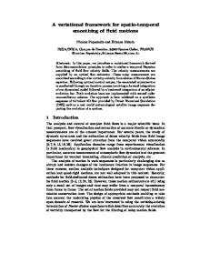
tion. More detail on the Ladybug camera system, pictured in Figure 2.3, is given in Section 5.1.

Figure 2.3: The Ladybug multi-sensor camera system [63]. The dense sampling approaches discussed above generally do not satisfactorily compensate for parallax when the amount of overlap between input images is less than fifty percent [48]. Simply applying stereo fusion in this situation results in discontinuities at the borders of the overlap regions. To avoid ghosting or echo artifacts when rendering sequences captured with the Ladybug, Kang et al. developed an algorithm called multi-perspective plane sweep (MPPS) [48]. The MPPS algorithm operates on pairs of input images, performing stereo matching in the overlap region, but also varying the view point for each pixel-column or group of columns in the overlapping region of the rectified input images. This is in contrast to standard stereo fusion where the viewpoint for the mosaic is located at a fixed point. For example, if rectified input images Iˆ0 and Iˆ1 overlap for N columns of pixels c0 , . . . , cN −1 , then the stereo correspondence for c0 is computed relative to the center of projection of Iˆ0 . For column cN −1 , dense stereo is computed relative to the center of projection of Iˆ1 , and the viewpoint is varied linearly in between. The overlap is then blended by a weighted average of the colors at corresponding pixels in the two images, and then projected back into the rectified images, overwriting the corresponding pixels. The weights are computed as a linear function of the distance of the pixel from the two edges of the overlap region. Figures 2.5 and 2.6 [48] illustrate the results of single-viewpoint fusion compared with the MPPS, respectively, for a pair of image captured using the Ladybug system. Notice the discontinuities in Figure 2.5 are removed in Figure 2.6. Instead, the wood beam is slightly bent in the overlap region compared with the non-overlapping regions, but this is a far less noticeable artifact than either the discontinuities, or the ghosting in Figure 2.4. The result is two images with different centers of projection, with the overlapping regions warped to account for parallax. The MPPS performs this task for each overlapping pair of

14

radially-oriented images; the top sensor is a special case and the top image must be fused with each radial image separately. The total result is six images with distinct centers of projection, and with regions warped to account for parallax with adjacent images. Rendering involves standard planar mosaicking and blending of these parallax-warped images. Uyttendaele et al. [49] use the Ladybug and the MPPS and other techniques to generate interactive image-based walk-through sequences of real-world environments.

Figure 2.4: Ghosting artifact from using direct blending and feathering of overlapping Ladybug images [48].

Figure 2.5: Discontinuities introduced by single-viewpoint stereo fusion in a small overlap setting [48]. The goal of this thesis is to compute a single, seamless panorama without ghosting or echo artifacts, with a single center of projection. While generating a panorama with a single

15

Figure 2.6: Ghosting in Figure 2.4 and discontinuities in Figure 2.5 are removed by the MPPS [48]. center of projection and then viewing it perspectively is equivalent to planar mosaicking of the parallax-warped images in the MPPS, this thesis is also motivated by the application of other computer vision algorithms to the resulting panoramas: eg. object detection, recognition and tracking, feature tracking and structure from motion, among others. Constraining the panoramic format to have a single center of projection avoids additional complications to the mathematics of these tasks, maintaining that similarity to their application to planar images. Applying such algorithms to the warped overlap images may be problematic, and resampling the images the extra time to generate the single-point-of-projection panorama will degrade image quality. While resampling may have an unremarkable impact for viewing, the effect on computer vision algorithms may yet be deleterious. Further, maintaining the high panoramic image quality gives more flexibility in how they are used. To obtain a seamless and artifact-free panoramic image, in this thesis a global optimization algorithm is used within a Bayesian framework. Specifically, Bayesian belief propagation is used on a Markov network. The Markov network contains loops, so the optimization is not strictly global, however it is optimal over very large neighborhoods in the solution space. These techniques are used to obtain dense correspondence between input images, in the form of depth from the panorama’s center of projection, from which to resample and blend the input images. Bayesian techniques leverage Bayes’ theorem: P (X|Y ) ∝ P (X) P (Y |X). The posterior probability of some unknown quantity X given some observed quantity Y , P (X|Y ), is computed in terms of an observed likelihood, P (Y |X) and a known, or approximated, prior probability on X, P (X). Here, a photoconsistency observation is used as the likelihood and a

16

smoothing prior is imposed by the Markov random field. In regions of the panorama covered by only one image, no photoconsistency observation can be made because colors from multiple images are needed to compute photoconsistency. This uncertainty is expressed by assigning a uniform distribution over depth in these regions. Fitzgibbon et al. [14] use a photoconsistency likelihood within a Bayesian framework for IBR. They enumerate local maxima of the likelihood by first densely sampling in depth; they compute photoconsistency at 500 depths for each output pixel. Then they find local maxima of the likelihood in color space by running gradient descent from multiple (≈ 20) random starting points in color space, and then clustering the results to obtain several local maxima. This process reduces the optimization to a discrete labeling problem. Instead of a smoothing prior, however, Fitzgibbon et al. use a texture prior. They extract a library of 5 × 5-pixel texture patches from the input images. The prior probability of an output pixel is then a Gaussian function of its distance to its nearest neighbor in the texture library. In their survey of image-based representations, Shum et al. [42] describe a continuum of IBR techniques based on the degree to which they incorporate geometric information. They partition the continuum into three categories of IBR techniques: those that use no geometry, those that use implicit geometry, and those that use explicit geometry. This thesis would fall near view interpolation [43] on the continuum, between techniques that use no geometry, such as the mosaicking techniques described above or concentric mosaics [45], and techniques that use implicit geometry, such as view morphing [44]. For more IBR techniques, the interested reader is referred to the survey of Shum et al. [42].

2.3

Markov Random Fields for Vision and Imaging

Let F be a field of discrete random variables sampled at a lattice Λ = (V, E), where V is the set of lattice sites with |V | = S, and E is the set of edges connecting them. Let each random variable Fs ∈ F for all s ∈ V have L possible values or labels f = 0, 1, . . . , L − 1, and denote a configuration by the vector of length S, f = [fs ∈ {0, 1, . . . , L − 1} ; ∀ s ∈ V ], such that F = f ↔ Fs = fs ∀ s ∈ V . Let the set of all possible configurations be denoted FSL . The field F is a Markov random field (MRF) if P (F = f) > 0 ∀ f ∈ FSL

(2.12)

and P (Fs = fs | {Fr = fr } ∀ r ∈ V, r 6= s) = P (Fs = fs | {Fr = fr } ∀ r ∈ N (s))

(2.13)

17

where N (s) ⊆ {r} : r ∈ V ; r 6= s is the neighborhood of s [2, 3, 6]. The first condition (2.12) is that all possible configurations have non-zero probability, however small, and the second (2.13) is Markov property itself, that the probability at a site s depends only on its Markov blanket, or neighborhood N (s). A Gibbs distribution on a field F is one of the form P (F = f) =

1 −U (f) e Z

(2.14)

where Z is a normalization constant called the partition function and U (f) is the energy of the configuration f. A clique is defined as subset C ⊆ V such that every pair of distinct sites s, r ∈ C are neighbors in Λ, i.e. (s, r) ∈ E. Notice that the neighborhood of a site is the union of the sites that share a clique with it: N (s) = {r ∀r : (s, r) ∈ E}. In this way, the edges represent statistical dependencies between the random variables in the Markov network. The energy function can be written X U (f) = UC (f) (2.15) C∈CΛ

where UC (f) is the energy or cost contribution from each clique in the set CΛ of all cliques in Λ for the configuration F [2, 6]. The clique energy is in fact a function of only the assignments or labelings Fs = fs for s ∈ C, and not the entire configuration. The Clifford-Hammersley theorem states that the field F is an MRF if and only if F can be described by a Gibbs distribution (2.14) [2, 3, 6]. From (2.15), the Gibbs distribution (2.14) can be rewritten as 1 Y −UC (f) 1 Y P (F = f) = e = φC (f) (2.16) Z C∈C Z C∈CΛ Λ

which gives a probability distribution corresponding to the energy function (2.15), where φC are probability distributions called clique potentials. Note that minimizing (2.15) and maximizing (2.16) are equivalent. Bayesian formulations are naturally well suited to vision and imaging problems: prior knowledge of the scene or image, and an observation (i.e. the input images, or a measurement computed from the input images) are used to estimate the posterior distribution of a property of the scene or image, given the observation. Bayes theorem states P (Y = y|X = x) P (X = x) = PL (Y = y|X = x) P (X = x) P (Y = y) (2.17) where X is the unknown random process (the quantity of the scene or image one wishes to estimate), and Y is the observed process. The posterior probability of X given the observation Y P (X = x|Y = y) =

18

is the product of the (normalized) observational likelihood PL (Y = y|X = x) = P (YP =y|X=x) (Y =y) and the prior distribution on X, P (X). The probability distribution of an MRF is completely described by its clique potentials, so an MRF that models the posterior distribution contains cliques that model the prior distribution and cliques that represent the observational likelihood. This is accomplished by taking an MRF FX that describes the prior distribution on the lattice ΛX = (VX , EX ), and “coupling” it
with an MRF FY |X that models the likelihood on ΛY |X = VY |X , EY |X . That is, adding either
edges, or sites and edges, to obtain FX|Y on ΛX|Y = VX|Y , EX|Y where VX|Y = VX ∪ VY |X and EX|Y = EX ∪ EY |X . The pre-eminent use of MRF models for imaging is the Bayesian restoration of images from Geman and Geman [2]. They use three coupled MRFs: the intensity process F on a pairwise or first-order lattice with sites Zm corresponding to the image pixels; a binary line process L (representing edges or discontinuities in the image) on the dual of the pixel lattice, Dm ; and they incorporate their observation field G through an image degradation model (blurring and noise) on a second-order lattice with the same sites, Zm , as the intensity field. The line and intensity fields interact such that for s, r ∈ Zm and d ∈ Dm between s and r, Usr (f) = 0 if Ld = 1. That is, if there is an edge or line between pixel sites s and r, then the clique energy is zero, regardless of the values of Fs and Fr . Otherwise Usr (f) is non-zero representing the “bond” between sites r and s. They also use a four-state line process, with state (label) 0 indicating no edge, and the other states indicating the orientation of the edge. The observation field is obtained without any additional sites, but by adding edges to create a second order neighborhood system on Zm , such that the neighborhoods modeling the statistical dependencies of the observation field correspond to the neighborhoods used as input to the image degradation model. The intensity field is the input to the degradation model, which is then compared to the observed degraded image to obtain a cost for the cliques of G. Konrad and Dubois [5] note that a vector field can have Markov properties as well as a scalar field (the only difference is the dimensionality of the state space of the field), and use this to apply the line field-coupled model of Geman and Geman to the Bayesian estimation of motion vector fields. Since motion estimation requires at least two images, they use an observation model on the probability of next image gt+ , given the previous image gt− and the estimated motion vector field dt : p (˜ gt+ |dt , lt , gt− ) ≈ e−Ug (˜gt+ |dt ,gt− ) , where g˜t+ is an interpolation of gt+ , lt is the line field, and Ug is the Gibbs energy for the observation field. That is, they assume the observation is independent of the line process. Using a displacement model of coupled motion and motion discontinuity fields (Dt , Lt ) they decompose the distribution according to Bayes’ theorem: p (dt , lt |gt− ) = p (dt |lt , gt− ) p (lt |gt− ). They note that the single

19

image frame will not contribute much information to the motion field and use an energy function independent of gt− : p (dt |lt , gt− ) ≈ e−Ud (dt |lt ) . They elegantly close the loop by modeling the line (motion discontinuity) field energy in terms of the previous frame: Ul (lt |gt− ), which is naturally computed in terms of the image gradient ∇gt− . Geiger and Girosi [3] use mean field approximation to average a surface field and a line field into a single field. They use this simplified model to reconstruct both intensity and depth surfaces. Black and Rangarajan [4] showed how the line field can be unified with outlier rejection through the use of robust statistics. They model the line process as an outlier process with respect to the smoothing prior, and similarly model outliers in the data (observation) field. They then show how these outlier processes can be approximated with robust estimators. More recently, Sun et al [12] use the robust estimation techniques of Black and Rangarajan to approximate a coupled disparity-line field for stereo. Now consider an MRF FΠ on a pairwise or first-order lattice Λ = (V, E) and a set Φ of potential functions on cliques in Λ. A first-order lattice, or graph, is one in which all cliques are 2-cliques, consisting of two sites. Further, let V be comprised of two subsets: sites {yp } represent observed random variables Y = {Yp }, and sites {xp } represent hidden quantities X = {Xp } of the scene, which we wish to infer, for every pixel p ∈ Π where Π is the panoramic image, or face of the cubic panorama, to be generated. Let Π consist of P pixels. The values or labels of FΠ represent candidate locations from which to resample the input images into panoramic form. These sampling locations are stored in the form of distances, or depths, from the panorama’s center of projection. In this case a configuration f = [x|G] for the P -element labeling vector x and the P × L   observation matrix G, where x = [fp ], and G = yp for all p ∈ Π. Each observation vector yp is of length L, and consists of a photoconsistency observation (cost), computed from the input images, for each labeling Xp = fp ∈ {0, 1, . . . , L − 1}. The assignment of a configuration to
the field then follows FΠ = f ↔ X = x ↔ Xp = fp , Y = G ↔ Yp = yp ∀ p ∈ Π. For every pixel p, (xp , yp ) ∈ E. The hidden nodes {x} are connected in a rectangular grid lattice such that (xp , xq ) ∈ E if and only if pixels p and q are non-diagonal neighbors in Π. Now, let the first potential function be the local evidence φ (xp , yp ) = P (Yp |Xp )

(2.18)

denoting the observational likelihood of Yp (i.e. that the input images could have been observed) given that a particular labeling of Xp is the correct one. Let the second potential function be the compatibility matrix ψ (xp , xq ) = P (Xp |Xq )

(2.19)

20

denoting the Markov prior probability of labeling xq given a labeling of xp . The clique potentials are the corresponding probability density functions
φp (fp ) = p Yp = yp |Xp = fp (2.20) denoting the likelihood of the local photoconsistency observation yp given the labeling Xp = fp , and ψpq (fp , fq ) = p (Xp = fp |Xq = fq ) (2.21) denoting the prior probability of the labeling Xp = fp given the labeling Xq = fq for hidden neighbors xp and xq . From (2.16), one can write the overall joint probability of all nodes in V as [2, 6, 11] Y Y P (X, Y ) = cX,Y ψ (xp , xq ) φ (xp , yp ) (2.22) (p,q)∈E

p∈Π

where cX,Y is a normalization constant and (p, q) is shorthand for the edge (xp , xq ). One can also write the posterior probability of the hidden quantities X given the set of observations Y as Y Y P (X|Y ) = cX|Y ψ (xp , xq ) φ (xp , yp ) (2.23) (p,q)∈E

p∈Π

cX,Y P (Y )

where cX|Y = is another normalization constant. Maximizing (2.22) is referred to as marginalization and results in the minimum mean squared error (MMSE) configuration fM M SE . Maximizing (2.23) results in the maximum a posteriori (MAP) configuration fM AP . For an individual variable Xp , the MMSE and MAP estimates are [1, 9] X X fpM M SE = fp p (X = x, Y = G) (2.24) fp

q∈Π,q6=p

and fpM AP = arg max max p (X = x, Y = G) fp

q∈Π,q6=p

(2.25)

respectively. From (2.14), (2.15), (2.16) and (2.23), the posterior probability of a configuration X = x given the observation Y = G can be written p (X = x|Y = G) = cX|Y e−U (x,G)

(2.26)

for the energy function U (x, G) =

X (p,q)∈E

Upq (fp , fq ) +

X p∈Π

Dp (fp )

(2.27)

21

where Upq (fp , fq ) and Dp (fp ) are the discontinuity cost and the data cost, respectively, such that ψpq (fp , fq ) = e−Upq (fp ,fq ) and φp (fp ) = e−Dp (fp ) . In fact, in this case the data cost can be taken as the photoconsistency observation itself: Dp (f ) = yp (f ) for f = 0, 1, . . . , L − 1, where yp (f ) is the scalar function returning component f of the observation vector yp . Thus, the probability of a photoconsistency observation being made (from the input images), given a
particular labeling fp of xp , is p Yp = yp |Xp = fp = φp (fp ) = e−yp (fp ) . However, the data cost notation, Dp (f ), will be used throughout this thesis, in keeping with precedent notation [13]. The maximum a posteriori labeling xM AP given the observation G can be computed by minimizing the energy, or “objective function”, (2.27). MRF formulations of early vision problems have existed for some time, exact evaluation of either the MMSE (2.24) or MAP (2.25) configuration is NP-hard, hence the need for approximation algorithms. Stochastic relaxation or simulated annealing approaches from statistical mechanics [2, 5] and mean-field approximation [3] among others have been used. Recently, considerable research has concentrated on the algorithms of graph cuts and belief propagation. Both graph cuts (e.g. [28]) and belief propagation estimate the MAP configuration. Tappen and Freeman performed a comparison of both algorithms as applied to the stereo problem [16] for MAP estimation using identical MRF parameters and found that results were generally comparable between the algorithms, although graph cuts found lower energy configurations. However, these lower-energy solutions were not necessarily closer to the ground-truth energies. In fact, the ground-truth energy was often significantly higher than both graph cut or BP due to pixels that did not match any in the other image. They subsequently concluded that improvements in MRF stereo algorithms will come from improvements to the MRF model rather than improvements in the optimization algorithm. All MRF formulations require the definition of parameters, such as weights for different potential functions, the values of which can dramatically affect the performance of the algorithm. The optimal values of these parameters often vary significantly from data set to data set, and often have to be hard-coded by trial and error. In their comparison of graph cuts and belief propagation, Tappen and Freeman use ten combinations of three parameters for each data set. Zhang and Seitz recently presented an expectation maximization (EM) approach to estimating optimal values for these parameters [18].

22

2.4

Bayesian Belief Propagation

The Bayesian belief propagation algorithm was originally introduced by Judea Pearl, in publications compiled into Probabilistic Reasoning in Intelligent Systems: Networks of Plausible Inference [1]. Belief propagation is run on a graph where the nodes represent random variables and the edges represent statistical dependencies between the variables the nodes represent. Beliefs, or probabilities of certain hypotheses given some evidence, are propagated through the network by local update rules. Pearl originally considered belief propagation for Bayesian networks, which are directed acyclic graphs, or trees, and on singly connected Markov networks, or Markov trees. This was because in such settings the algorithm gives an exact solution, and because Pearl was considering the algorithm as applied to diagnostic and decision making systems, not imaging and vision. However, loopy belief propagation, has since had both empirical success and theoretical justification in finding approximately optimal solutions on Markov networks with cycles. Section 2.4.1 describes the two variants of belief propagation as originally developed by Pearl for Bayesian networks. Section 2.4.2 then discusses how belief propagation works on singly-connected Markov networks, or Markov trees. Section 2.4.3 follows with a discussion of how belief propagation can be used as an approximation algorithm on MRFs that contain loops, such as regular image grid lattices, and its subsequent application to vision and imaging problems.

2.4.1

Belief Updating and Belief Revision on Bayesian Networks

Pearl developed two algorithms, belief updating and belief revision, which are now both considered variants of the same algorithm, belief propagation. First, consider belief updating on a causal tree (Bayes net), where an edge from node X to node Y explicitly represents the causal dependency of Y upon X. The belief distribution of node X can be computed if the following parameters are available:
1. The causal support of X, from its parent U : πX (u) = P u|e+ X .   − 2. The diagnostic support of X, from the j-th child of X, Yj : λYj (x) = P eYj |x . 3. The fixed conditional probability P (x|u) relating X to its immediate parent U . + Here, e− X stands for the evidence contained in the tree rooted at X, and eX stands for the evidence contained in the rest of the network. The lower-case x and u represent specific values

23

of the variables X and U , respectively. Pearl also extended this algorithm to causal polytrees: Bayesian networks where node X may have multiple causal parents Ui . The first quantity above, πX (u), is the message received by X from its parent U . The second quantity, λYj (x), is the message received by X from its j-th child Yj . The third quantity is a matrix expressing the compatibility of an assignment X = x with the assignment to the immediate parent U = u, and is equivalent to the Markov prior potential, or compatibility matrix ψ, described in Section 2.3. Belief updating proceeds by performing three steps at each node in the network: belief updating, bottom-up propagation, and top-down propagation. Belief updating for node X involves inspecting the parameters listed above and updating at X its belief BEL (x) = αλ (x) π (x) (2.28) where λ (x) =

Y

λYj (x)

(2.29)

P (x|u) πX (u)

(2.30)

j

and π (x) =

X u

and α is a normalizing constant such that the beliefs sum to 1 over x. In bottom-up propagation, node X computes, for each possible value u of U , the message X λ (x) P (x|u) (2.31) λX (u) = x

and sends it to the parent node U . In top-down propagation, X computes, for each possible value x of X, the message Y πYj (x) = απ (x) λYk (x) (2.32) k6=j

and sends it to the child node Yj . These steps are run over the entire network. The update formulas (2.28), (2.31) and (2.32) preserve the probabilistic meaning of the messages and beliefs such that after at most one global iteration
λX (u) = P e− (2.33) X |u ,
πY (x) = P x|e+ (2.34) Y and BEL (x) = P (x|e)

(2.35)

24

− where e = e+ X ∪ eX is the total evidence in the network [1, 9, 7]. That is, the belief at node X is the marginal probability of X, given all the available evidence. One global iteration simply means that all three steps are performed for every node in the network. Belief revision is identical to belief updating, except that the summations in (2.30) and (2.31) are replaced by maximizations. Hence, the two algorithms became known as the “sumproduct” and “max-product” variants of Bayesian belief propagation, respectively. The best explanation of the conceptual difference between the two comes directly from Pearl (p. 240):

. . . belief updating, i.e., assigning to each hypothesis in a network a degree of belief BEL, which changes smoothly and incrementally with each new item of evidence. This chapter applies Bayesian analysis and belief networks to another task: revision of belief commitments, where by belief commitment we mean the categorical but tentative acceptance of a subset of hypothesis that together constitute the most satisfactory explanation of the evidence at hand. In probabilistic terms, that task amounts to finding the most probable instantiation of all hypothesis variables, given the observed data. The resulting output is an optimal list of jointly accepted propositions, a list that may change abruptly as more evidence is obtained. In the terminology of Section 2.3, the sum-product algorithm computes the MMSE configuration, or marginalization, of the network, while the max-product algorithm computes the MAP configuration of the network. The probabilistic meanings of the messages and beliefs in belief revision, or max-product belief propagation, are slightly different than their counterparts in belief updating, or sumproduct belief propagation. Let W stand for the set of all variables considered, including those in e, and call any assignment w to the variables in W that is consistent with e an extension or explanation of e. The most probable explanation (MPE) of e is the extension W = w∗ that maximizes the conditional probability p (w|e). The revised belief of an assignment X = x is the probability of the most probable extension of e that is also consistent with the assignment X = x [1] BEL∗ (x) = max p (x, w0x |e) (2.36) 0 wx

W0X

where = W − X; that is all other variables besides X. The MAP assignment for X is the one that maximizes (2.36). The messages obtain the following probabilistic meanings:
(2.37) p w− λ∗X (u) = max U X |u − wU X

is the conditional probability of the most probable assignment to all the variables in the subgraph rooted at X, w− U X , given the assignment U = u. That is, it is the probability of the MPE

25

− of e− U X , given the assignment U = u. The notation eU X comes from the extension to causal polytrees, where the node X might have multiple causes Ui : i = 1, 2, . . . , and is equivalent to the e− X notation for causal trees. And,

πY∗ (x) = max p x, w+ X0Y +




(2.38)

wX 0 Y

is the maximum joint probability of the assignment X = x and the assignment of all variables in the graph “above” Y , excluding X, w+ X0Y .

yp φp ψpq

xp

φq xq

ys

ψps xs

yq

φs

Figure 2.7: A singly connected MRF of three hidden nodes and three observed nodes.

2.4.2

Belief Propagation on Markov Trees

Now consider belief propagation on a singly connected Markov network, such as Figure 2.7, which shows a simple, singly connected MRF corresponding to a three-node segment of X and the corresponding nodes of Y from the MRF FΠ described in Section 2.3. The local message passing rules are in fact simpler for singly connected Markov networks than for Bayesian networks, because the edges in the Markov graph are undirected they do not imply any causal dependence, and hence there is no need for π-messages. Thus there is only one type of message, λ-messages. By substituting into (2.22), we get the joint probability of the network as P (Xp , Xq , Xs , Yp , Yq , Ys ) = ψ (xq , xp ) ψ (xs , xp ) φ (xp , yp ) φ (xq , yq ) φ (xs , ys )

(2.39)

26

which can then be substituted into (2.24) or (2.25) to solve directly for fpM M SE or fpM AP , respectively. For example, fpM AP = arg max max max ψqp (fq , fp ) ψ (fs , fp ) φp (fp ) φq (fq ) φs (fs ) fp

fq

fs

= arg max φp (fp ) max ψqp (fq , fp ) φq (fq ) max ψsp (fs , fp ) φs (fs ) fp

fq

fs

(2.40)

is the MAP labeling of xp in Figure 2.7.

xp

ψps

ψpq xq

xs φs ys

φp yp

φq yq

Figure 2.8: The Markov network in Figure 2.7 as a tree rooted at xp . However, as discussed in Section 2.3, the Markov networks required to solve most realworld problems are large enough to make exact calculations such as above infeasible. For example, the MRF FΠ has 2 million nodes in most experiments conducted for this thesis. Instead, approximation algorithms are used to estimate the marginal and posterior distributions. While (2.16) is true for general Markov networks, an additional factorization is valid for Markov chains and Markov trees, which leads to a message passing approximation algorithm that estimates either the marginals (2.22) or the posterior (2.23). Figure 2.8 shows the network in Figure 2.7 as a tree rooted at node xp . Using the Markov properties, one can write the joint probability as [1, 9] P (Xp , Xq , Xs , Yp , Yq , Ys ) = P (Xp ) P (Yp |Xp ) P (Xq |Xp ) P (Yq |Xq ) P (Xs |Xp ) P (Ys |Xs ) which is the same as (2.39), and is a chain rule factorization of the joint probability [1, 9]. One

27

can rewrite (2.40) as fpM AP = arg max p (Xp = fp ) mpp (fp ) mqp (fp ) msp (fp ) fp


where the message from yp to xp is mpp (fp ) = p Yp = yp |Xp = fp = φp (fp ) because yp is a leaf node [1]. Making a similar observation for yq and ys , The message from xq to xp is then
mqp (fp ) = max p (Xq = fq |Xp = fp ) p Yq = yq |Xq = fq = max ψqp (fq , fp ) φq (fq ) fq

fq

and similarly for msp . Without single-node a priori potentials, one can take the prior on xp by itself as the uniform distribution p (Xp = fp ) = 1 ∀fp . This allows fpM AP to be rewritten as fpM AP = arg max φp (fp ) mqp (fp ) msp (fp ) fp

which evaluates to (2.40) upon substitution. If one then considers the Markov network in Figure 2.7 as a tree rooted at node xq , one can perform a similar factorization and write the MAP labeling Xq = fqM AP as fqM AP = arg max φq (fq ) mpq (fq ) fq

where mpq (fq ) = max φp (fp ) ψpq (fp , fq ) msp (fp ) fp

which by substitution gives fqM AP = arg max φq (fq ) max ψpq (fp , fq ) φp (fp ) max ψsp (fs , fp ) φs (fs ) fq

fs

fp

which is analogous to (2.40). This example shows a method for computing the MAP assignment for each variable in a singly connected network in terms of local message passing rules. These rules generalize to Y fpM AP = arg max φp (fp ) mqp (fp ) (2.41) fp

q∈N (p)

for the MAP label of Xp and mpq (fq ) = max ψpq (fp , fq ) φp (fp ) fp

Y

msp (fp )

(2.42)

s∈N (p)\q

is the message from node xp to xq , i.e. when solving for fqM AP ; and N (p) denotes the hidden neighbors of xp , i.e. the first-order neighborhood of xp excluding yp . Hence, N (p) \q is the

28

first-order neighborhood of xp excluding yp and xq , where the notation S\s indicates the set S excluding the element s. One can also note that these messages are equivalent to the λ∗ -messages from belief revision on a Bayesian network. Since the above passage derived the messages for the maxproduct algorithm using the Markov properties of the network, the derivation from diagnostic messages will be done for the sum-product algorithm (i.e. from the λ-messages). Without causal dependence between nodes, one can consider all messages as diagnostic  messages and derive the message update formula from (2.31). The message λyp (f ) = p e− yp |Xp = fp is the diagnostic support of xp from the child node yp , X

X λyp (Xp = fp ) = λ yp p yp |fp = φp (fp ) = φp (fp ) (2.43) yp

yp


from (2.20), because yp is fixed for a particular set of input images, and because λ yp = 1 since yp is a leaf node [1]. The diagnostic support message sent to a hidden node xq from its hidden neighbor xp is X p (Xp = fp |Xq = fq ) λ (Xp = fp ) . λxp (Xq = fq ) = fp

By noting that ψpq (fp , fq ) = p (Xp = fp |Xq = fq ) (2.21) and by extending (2.29) such that Y λ (Xp = fp ) = λv (Xp = fp ) v:(xp ,v)∈E,v6=xq

where v denotes each neighbor of xp other than xq , one can write X Y λxp (Xq = fq ) = ψpq (fp , fq ) λv (Xp = fp ) fp

v:(xp ,v)∈E,v6=xq

which becomes λxp (Xq = fq ) =

X

Y

ψpq (fp , fq ) φp (fp )

fp

λxs (Xp = fp )

s∈N (p)\q

because λyp (Xp = fp ) is constant from (2.43). In the notation of (2.42) the message is written X Y mpq (fq ) = ψpq (fp , fq ) φp (fp ) msp (fp ) (2.44) fp

s∈N (p)\q

and the MMSE estimate Xp = fpM M SE X Y fpM M SE = fp φp (fp ) mqp (fp ) fp

q∈N (p)

(2.45)

29

is the expected value of Xp given all the nodes in the network. It can be shown [1, 7], that for singly connected Markov networks after at most one global iteration of (2.42) for each node in the network, (2.41) gives the globally optimal MAP estimate.

2.4.3

Loopy Belief Propagation for Vision and Imaging

Both the sum-product and max-product algorithms are guaranteed to converge to exactly optimal solutions for graphs without loops, where loops are undirected cycles in the network (directed loops are by definition not permitted in Bayesian networks) [1]. The introduction of loops into the network may violate the conditional independence assumed among a node’s ancestors [1] (p. 195): If we ignore the existence of loops and permit the nodes to continue communicating with each other as if the network were singly connected, messages may circulate indefinitely around these loops, and the process may not converge to a stable equilibrium. . . . Such oscillations do not normally occur in probabilistic networks because of the stochastic nature of the link matrices, which tend to bring all messages toward some stable equilibrium as time goes on. However, this asymptotic equilibrium . . . does not represent the posterior probabilities of all nodes in the network. The reason for this is simple: all of our propagation equations were based on some conditional independence assumptions that might be violated in multiply connected networks. Nonetheless, both the sum-product and max-product (and equivalent min-sum) algorithms have been applied with success to pairwise image-lattice MRFs, which have many loops. This is the model used in this thesis. Examples include [9, 12, 13, 15]. Belief propagation on graphs with loops is known as loopy belief propagation, but is often simply called belief propagation. On graphs with loops, belief propagation produces solutions that are optimal over large neighborhoods of the solution space. In [8], Weiss and Freeman proved that for an arbitrary graphical model, solutions produced by the max-product algorithm were maxima of single loops and trees (SLT) neighborhoods of the configuration. The SLT neighborhood of a configuration x∗ includes all configurations x that can be obtained from x∗ by selecting an arbitrary subset of nodes in the graph that consists of disconnected combinations of trees and single loops, and assigning arbitrary values to those nodes.

30

Intuitively, the singly connected restriction ensures that each piece of evidence is only counted (propagated) once per MAP or MMSE estimate. In a graph with loops, evidence will be counted multiple times [7] (“messages may circulate indefinitely around these loops”). However, Weiss showed that on a “balanced” loopy network, although evidence is counted more than once, all evidence is “double counted” equally [7]. An “unwrapped network” of a loopy network is a singly connected network, constructed from a loopy network by replicating nodes and edges, such that performing belief propagation on the unwrapped network is equivalent to performing it on the loopy network. The loopy network is considered balanced if one can construct an unwrapped network such that all nodes and edges are replicated an equal number of times. Loopy belief propagation, in contrast to a singly connected network, requires more than one global iteration to converge. To reduce subscripts for the sake of clarity, the convention in the following will be that f represents the labeling of xp and g represents the labeling of xq . The message at iteration t from node xp to xq is the vector mtpq of length L, with each component being proportional to how likely node xp “believes” it is that node xq will have the label corresponding to that component. Let the scalar function mtpq (g) denote the message vector component corresponding to label g. After T iterations, a belief vector bp is computed for each hidden node xp , where each component bp (f ) represents the probability that Xp = f given the evidence in the network. In the sum-product algorithm, messages are computed as follows [10, 11] Y X ψpq (f, g) φp (f ) mt−1 (2.46) mtpq (g) = κ1 sp (f ) . f

s∈N (p)\q

where κ1 is a normalization constant. In the max-product algorithm messages are updated in the following way [12, 16, 8] Y (2.47) mtpq (g) = κ2 max ψpq (f, g) φp (f ) mt−1 sp (f ) f

s∈N (p)\q

where κ2 is a normalization constant. After T iterations, in both the sum-product and maxproduct algorithms, the beliefs are computed [12, 8, 10, 11] Y bp (f ) = κ3 φp (f ) mTqp−1 (f ) (2.48) q∈N (p)

and the MAP and MMSE labeling for node xp are fpM AP = arg max bp (f ) f

(2.49)

31

and fpM M SE =

X

f bp (f ) ,

(2.50)

f

respectively. The max-product algorithm can also be converted to the “min-sum” algorithm, which minimizes the energy function (2.27), by taking the negative of the logarithm of the message and belief probabilities. The min-sum algorithm is equivalent to the max-product algorithm; the messages and beliefs are computed in energy space, rather than probability space. Hence, the maximization of a product of probabilities in the max-product algorithm becomes a minimization of a sum of energies, and the message updates become [13]   X , (2.51) mtpq (g) = min Upq (f, g) + Dp (f ) + mt−1 sp (f ) f

s∈N (p)\q

the beliefs become bp (f ) = Dp (f ) +

X

mTqp−1 (f )

(2.52)

q∈N (p)

and the MAP label is found by fpM AP = arg min bp (f ) . f

(2.53)

In this thesis, the min-sum formulation of the max-product loopy belief propagation (BP) algorithm is used to minimize the energy function (2.27) corresponding to the posterior distribution (2.23). This is done mostly for numerical concerns; multiplication of floating point numbers is generally less stable than addition. Also, the algorithm used in this thesis is based on that of Felzenzswalb and Huttenlocher [13], who use the min-sum version. Freeman et al. [9] apply loopy BP to a number of low-level vision problems, primarily super-resolution. That is, estimating high-resolution detail from a single low-resolution image. (This is distinct from image-sequence super-resolution, which estimates high-resolution detail from multiple low-resolution images.) They define the nodes of their MRF to correspond to image patches: hidden nodes correspond to scene, or high-resolution, patches and observed nodes to patches in the low-resolution image. The scene patches are spaced so that they overlap, and the compatibilities are computed as the agreement between the pixels of neighboring patches which overlap. Specifically, they assume a Gaussian distribution on the difference of the overlapping pixels in the two patches. The candidate scene patches are obtained by finding the best L matches to the low-resolution image patches in a training database of image patches associated with high-resolution scene patches. The distance between each associated image

32

patch and the observed image patch estimates the local evidence. Yedidia et al. introduced Generalized Belief Propagation (GBP) [10, 11]. They construct messages between groups of nodes by building a hierarchy of regions (connected groups of nodes) by their intersections, such that a message is sent from a region to each of its direct sub-regions. A sub-region s of a region r is a direct sub-region if s is not also a sub-region of another sub-region s0 of r. If r and r0 are four-node regions (eg. on a pair-wise lattice) that overlap in the region s = {u, v} where u and v are nodes in the lattice, then messages will be sent from both r and r0 to s. On a pair-wise lattice, r and r0 are straightforwardly constructed such that u and v are neighbors. This could be considered a way of “unwrapping” or “loosening” the loops in the network in terms of the way the messages are passed, and the “significant” improvement over standard belief propagation for 2D pair-wise lattices [11] is certainly related to the theoretical results of Weiss [7], and Weiss and Freeman [8]. Since BP is an iterative algorithm, improving its efficiency primarily involves finding ways to either reduce the number of iterations needed or to reduce the amount of computation required for each iteration. Sun et al. [12], in applying loopy BP to the dense stereo problem, achieve a speed-up in the propagation step by about 30-60 percent by observing that each row of the compatibility matrix is a unique peak distribution and that most messages form distributions with a unique peak. The product of two unique peak distributions itself has a unique peak, which lies between the peaks of the first two. This fact can be used to eliminate unnecessary multiplications. Further, Sun et al. [12] use the line and outlier field unification of Black and Rangarajan [4] on their three coupled MRFs (disparity, line, and observation). By using robust statistics to approximate an outlier process for both the observation and line fields, they effectively handled both depth discontinuities and occlusions. They also illustrate the straightforward incorporation of additional cues into BP by adjusting the compatibility matrix ψpq if pixels p and q are in different segments. By combining robust statistics with image segmentation they developed a stereo algorithm that was demonstrably one of, if not the most accurate at the time. As noted in this section and in Section 2.3, graphical models incur significant storage and computational complexity. Running time for belief propagation is O (T L2 S), where T is the number of iterations, L is the number of labels, and S is the number of sites in the MRF lattice. The quadratic relationship of the running time to the number of labels, or states, of each node is particularly prohibitive toward high-dimensional or large state-space fields. Tappen et al. [15] overcome this by using a set of trained linear regressors as their set of labels to model a field with a much larger state space than the number of regressors (labels). They apply this technique to both super-resolution and Bayer tile color demosaicking, where the fields have

33

ranges equal to the number of desired intensity (color channel) levels, typically 256. Felzenszwalb and Huttenlocher [13] presented three algorithmic techniques to substantially improve the running time of BP for low-level vision problems. These techniques will receive further exposition in Section 3.2 as they are applied to the resampling of input images into a panorama. First, they noted that for early vision problems, such as stereo, the compatibility matrix is often a function only of the difference between the two labels, as opposed to the actual values of the labels. This leads to a message updating scheme, as described in Section 3.2, that is linear in L instead of quadratic in general. Second, a four-connected image grid graph is a bipartite graph. That is, {xp } can be partitioned into two subsets A and B such that any node xa ∈ A has only neighbors xb ∈ B. Colouring X in a checkerboard pattern and taking A to be one colour and B as the other is such a partition. Given the messages sent from nodes in A at iteration t, we can compute the messages sent from nodes in B at iteration t + 1, and in turn the messages sent from nodes in A at iteration t + 2 without ever computing the messages sent from nodes in A at iteration t + 1. This means only half the messages need to be updated each iteration. Third, they use a “multiscale” or hierarchical scheme for coarse-to-fine MAP estimation. Messages are typically initialized to the uniform distribution, that is zero in the min-sum version, but if they are initialized closer to their point of convergence, they should take fewer iterations to converge. This is achieved by defining nodes in level k + 1 to be the aggregation of four spatial neighbors in level k. The BP algorithm is then iterated at higher levels first, and the resulting messages are used as initial values for messages between the child nodes in next (lower) level. Finding the globally optimal solution to the Gibbs energy of a 2D pair-wise MRF is generally NP-complete [28]. However, under easily verifiable conditions, which are met for standard stereo benchmark data sets, a variant of the BP algorithm gives the global optima [17]. Tree reweighted belief propagation (TRBP) is a special case of GBP. The global minimum of an energy function of the same form as (2.27) does not improve many of the inaccuracies in the BP or graph cut solutions (to the stereo problem), suggesting that the problem is not the optimization algorithm, but rather the energy function itself [17]. Tappen and Freeman similarly concluded in their comparison of graph cuts and BP for stereo that performance improvements will come from improving the model of the MRF, not by improving the optimization algorithm, noting that both graph cuts and BP found configurations with significantly lower energy than that of the ground truth disparities [16]. For the Middlebury benchmark [51], between approximately 60 and 80 percent of the energy of the ground truth solution was due to high matching costs of occluded pixels [16].

34

One way to improve the model is to incorporate additional cues, eg. segmentation [12]. The use of robust estimators to incorporate outlier processes is also an improvement of the model [12]. Since appearing, the work of Felzenszwalb and Huttenlocher [13] has been a popular vehicle for extending BP and applying it to improved models, due to their techniques’ simplicity and efficiency. At CVPR 2005, five contributions [19, 20, 21, 22, 23] related directly to belief propagation, plus the expectation maximization technique for MRF parameter estimation [18]. Williams et al. [20] use a 3D MRF to estimate both stereo and motion in a stereoscopic video sequence using belief propagation, and cite as future work the use of efficient low-level vision techniques for BP [13] to improve the running time of their algorithm. They couple a 2D disparity field with a temporal field for motion to obtain a 3D MRF with compatibility functions between: hidden and observed nodes at time τ , spatially neighboring hidden nodes at time τ , and hidden nodes at the same spatial location at time τ and time τ − 1. The following year, several more CVPR contributions related directly to belief propagation, including [24, 25, 26, 27]. In [24], a hierarchical BP technique similar to Felzenszwalb and Huttenlocher [13] is used, along with other techniques, to achieve one of the best stereo results to date. Zhang et al. [25] use efficient BP for early vision [13] to solve a disparity or optical flow MRF coupled with an Illumination Ratio Map (IRM) MRF to perform stereo or tracking robustly under variable illumination. They note that if one field is fixed, BP can be used to solve for the other. Hence, they alternately fix the IRM field and solve for the disparity (optical flow) field, and vice versa. This is similar to the technique of Konrad and Dubois [5] in alternately solving for motion and motion discontinuity fields, and the Iterated Conditional Modes (ICM) [59] method used by Fitzgibbon et al. [14] to alternately optimize the photoconsistency likelihood and texture prior for image-based rendering. A preliminary version of this thesis appeared at the Third International Symposium on 3D Data Processing, Visualization and Transmission (3DPVT) in June 2006 [60].

Chapter 3 Belief Propagation for Panoramic Imaging of Complex Scenes In this thesis, loopy Bayesian belief propagation is used to estimate the maximum a posteriori (MAP) panoramic image given a set of input images taken from various positions and orientations surrounding the desired center of projection for the panorama. To generate each pixel in the panoramic image, the input images are resampled at the estimated MAP locations corresponding to that pixel. Each pixel in the panorama corresponds to a direction from the center of projection of the panorama, and corresponding sampling locations in the input images are computed by back projecting to some depth and reprojecting the resulting 3D point into the input images. (Input images from which the point is not visible are ignored.) Thus, estimating the MAP panoramic image requires estimating the MAP depth at each pixel in the panorama. The MAP depth will be computed as the MAP configuration fM AP of the MRF FΠ described in Section 2.3, such that it minimizes the energy function (2.27). When estimating the MAP depth across the pixels in a panoramic image using a Bayesian framework, the first task is computing the observational likelihood that the input images were generated given a particular depth assignment to each pixel. This is also known as the local evidence for each pixel. At each pixel, by measuring photoconsistency at a set of L depths z (f ) for f = 0, 1, . . . , L − 1 one can observe the likelihood that the images were generated given the scene has depth z (f ) at that pixel, or φp (f ) as in (2.20). Section 3.1 describes computation of the data cost. The second task is to impose a Markov smoothing prior on the likelihood to obtain the MAP scene depth and hence the MAP sampling of the input images. This is done using a highly efficient modification of loopy BP for early vision [13], as described in Section 2.4.

35

36

Section 3.2 describes the algorithm in greater detail. The third task is to resample the input images using the MAP sampling, which is described in Section 3.3. Generating a cubic panorama involves generating six planar perspective views, one for each face. MAP resampling can be adjusted to constrain the views to be consistent where they meet, and avoid seams along the edges of the cube.

3.1

Image Sampling and Data Cost Calculation

For each pixel p in the panorama, the data cost for each label f = 0, 1, . . . , L − 1 is computed by first back projecting along that pixel’s direction to some depth z (f ) obtaining the 3D point Pf . The visibility function of Pf in image j is Vj (Pf ) = 1 if it is visible, and 0 otherwise. Dropping the subscript f for clarity, the projection of P into image j is pˆj and the colour resulting from sampling image j at pˆj is cj (ˆ pj ). Then, the colour of pixel p for label f is the weighted mean of the colour samples from the input images from which the point P is visible cp (f ) =

1 X Vj (P) wj (ˆ pj ) cj (ˆ pj ) W j

(3.1)

where wj (ˆ pj ) is a weight based on the distance of the reprojection from the center of projection of image j and W is the total weight across all visible images. Let r (ˆ pj ) be the distance of pˆj from the optical center of image j and rbound (ˆ pj ) be the distance from the same to the edge of the image passing through pˆj . Then, the weight is wj (ˆ pj ) = rbound (ˆ pj ) − r (ˆ pj ). The colour computed in (3.1) is used as the reference colour for computing the photoconsistency of each pixel p. That is, the data cost is the photoconsistency or similarity of the input images with respect to the weighted mean, as opposed to the similarity of each input image with respect to every other input image. One possible measure for the data cost is the single-pixel variance of luminances Dp (f ) =

1 X Vj (P) wj (ˆ pj ) (¯ cj (ˆ pj ) − c¯p (f ))2 W j

(3.2)

where c¯j (ˆ pj ) and c¯p (f ) are the scalar luminances of the RGB colours cj (ˆ pj ) and cp (f ), respectively. An extension of this is to sum over a window Ω (p) centered on p Dp (f ) =

X X j

q∈Ω(p)

1 Vj (Q) wj (ˆ qj ) (¯ cj (ˆ qj ) − c¯q (f ))2 Wq

(3.3)

37

where Wq is the total weight over all input images for pixel q. Experiments for this thesis include data cost computations using (3.2) and (3.3) with a 5 × 5 window. In [52], Birchfield and Tomasi introduced a pixel dissimilarity measure that is insensitive to the effects of image sampling inconsistencies that occur between any pair of images. They symmetrically define the dissimilarity of a pixel p0 in image I0 and a pixel p1 in image I1 as  d (p0 , p1 ) = min d¯(p0 , p1 , I0 , I1 ) , d¯(p1 , p0 , I1 , I0 ) . These symmetric quantities are defined ¯ ˆ d (p0 , p1 , I0 , I1 ) = min I0 (p0 ) − I1 (q) 1 q∈ 2 (p1 )

and correspondingly for d¯(p1 , p0 , I1 , I0 ), where 21 (p1 ) denotes the square window extending one half-pixel from p1 along both axes, I0 (p) is the result of sampling I0 at pixel p, and Iˆ1 (q) is the linear interpolation at sub-pixel location q of I1 . Kolmogorov and Zabih [53] extend this to colour images by averaging the dissimilarity over the colour channels. In this thesis, the asymmetric dissimilarity of each input image with respect to the weighted mean (3.1) dp,j (f ) = min |cj (ˆ pj ) − cp (f )| (3.4) 1 q∈ 2 (ˆ pj )

is used to compute a third version of the data cost used in experiments for this thesis. This dissimilarity is averaged over the colour channels [53] and then summed over the visible input images   X 1 1 1 Dp (f ) = Vj (P) · dp,j . (3.5) 3 3 3 j Experiments were not conducted using the symmetric dissimilarity [52, 53], however this would be an interesting future experiment. Equations (3.2), (3.3) and (3.5) give three ways of computing a photoconsistency observation, or data cost, given a specific pixel p, label f and depth associated with that label z (f ). However, this begs the question of what depth to associate with a given label. Simple planesweep techniques sample at one depth for each label, over all pixels, as shown for a face of a cubic panorama in Figure 3.1. Figure 3.2 shows a simple example of choosing depths zp (f ), for each label f . The data cost, Dp (f ) is computed by reprojecting p into the input images (from which it is visible) from depth zp (f ), as shown in Figure 3.3, and then computing the pixel dissimilarity (3.5). The labels’ depths might be linearly spaced over a chosen depth interval, eg. Figures 3.2 and 3.3, or might be chosen based on prior knowledge of the scene or imaging process. A more robust method is to associate each label with a depth that results in an approximate local minimum of the data cost. As described in Section 2.2, Fitzgibbon et al do this in colour

38

space using gradient descent [14]. In this thesis, each label is associated with a sub-interval of a “global” interval in depth space. The sub-intervals are equal in length and contiguous. By sampling at multiple depths within its sub-interval, each label is associated with an approximate local minimum. This thesis uses a simple hierarchical multi-sampling technique that results in a sampling period (distance between nearest samples) Ts = 2−Ks ∆z, where ∆z is the baseline depth increment (distance between centroids in successive intervals) and Ks is the number of levels in the sampling hierarchy. The hierarchical sampling proceeds by sampling at the interval centroid (sampling level 0), splitting the interval into two and sampling at the centroids of those intervals (level 1), splitting each of them into two and sampling, and so on until level Ks − 1, always maintaining the sample with the minimum photoconsistency cost zˆp (f ) for each pixel p, within the label’s interval. This technique, illustrated for Ks = 4 in Figure 3.4, simply provides a denser exhaustive sampling in depth, without increasing the number of labels needed for the MRF.

Figure 3.1: Plane-sweeping for a face of a cubic panorama.

39

Y Z

yp

zp (0)

zp (1)

f =0

zp (2)

f =1

f =2

Figure 3.2: Depth sampling associated with the observation node yp of panoramic pixel p.

3.2

Efficient Belief Propagation for Panoramic Imaging

As noted in Section 2.4, Felzenzswalb and Huttenlocher [13] developed a highly efficient version of the min-sum loopy belief propagation algorithm for low-level vision problems, which we use with minor modifications to minimize the energy function (2.27). Section 3.1 described the different methods used in this thesis for computing the data cost. The other term in (2.27) is the discontinuity cost, for which we use the truncated linear model Upq (f, g) = min (λ kf − gk , dpq )

(3.6)

where λ is a scale parameter and dpq is the truncation threshold of the discontinuity cost between pixels p and q. In most experiments dpq = d is constant over the field, however it could be made dependent on edge or similar processes. It was observed [13] that discontinuity costs like (3.6), that depend only on the difference between the labels f and g and not the specific values of f and g, allow for a two-pass message update algorithm that is linear in the number of labels L. Generally, message updates are O (L2 ) because Upq (f, g) must be evaluated at every label f (of xp ) for every label g (of xq ). The last two terms of the message update formula (2.51) can be combined into a single term such that (2.51) becomes mtpq (g) = min (Upq (f, g) + hpq (f )) f

where hpq (f ) = Dp (f ) +

X s∈N (p)\q

mt−1 sp (f ) .

(3.7)

40

Y Z I0

yp I1

Dp (0)

Dp (1)

Dp (2)

f =0

f =1

f =2

Figure 3.3: The data cost Dp (f ) associated with node yp is made by reprojecting pixel p into the input images (I0 and I1 ) from depth zp (f ). From (3.6) it is clear that Upq (f, g + 1) = Upq (f, g) + λ for g ≥ f (and λ |g + 1 − f | ≤ dpq ), and hence Upq (f, g + 1) + hpq (f ) = Upq (f, g) + hpq (f ) + λ. Given this, the observation that Upq (f, f ) = 0, the fact that hpq (f ) is constant over g, and the fact that the message vector components mtpq (g) are minimized over f , it is clear that 1. mtpq (g) ≤ hpq (g) 2. mtpq (g) ≤ mtpq (g − 1) + λ (for g > 0) 3. mtpq (g) ≤ mtpq (g + 1) + λ (for g < L − 1) 4. ming hpq (g) ≤ mtpq (g) ≤ ming hpq (g) + dpq which leads directly to the following two-pass algorithm. The message vector components are evaluated sequentially over the labels in a forward pass for f = 0, 1, . . . , L − 1 mtpq (f ) = {

hpq (f )
min hpq (f ) , mtpq (f − 1) + λ

If f = 0 otherwise

(3.8)

followed by a backward pass for f = L − 1, L − 2, . . . , 0 mtpq (f ) = min mtpq (f ) , mtpq (f + 1) + λ mtpq

 (f ) = min

mtpq




(3.9)

 (f ) , min hpq (g) + dpq g

(3.10)

41

label:

f

2−Ks ∆z z

f +1

∆z

Figure 3.4: Hierarchical multi-sampling technique with Ks = 4. The dots indicate depths at which samples are taken from the input images. where (3.9) is analogous to the forward pass (3.8) and (3.10) applies the truncation threshold for the discontinuity cost (3.6). This algorithm is depicted for a hypothetical message in Figure 3.5. A simple three label example is depicted in Figures 3.8, 3.9 and 3.10. Figure 3.8 shows how the intermediate quantities hpr (g) are computed from the incoming messages mup , mlp , mdp , and the data cost Dp . Figures 3.9 and 3.10 show how the outgoing message vector is modified after the forward and backward passes, respectively, for discontinuity cost scale λ = 1. Felzenzswalb and Huttenlocher also observed that a four-connected image grid (one node for each pixel, edges between horizontal and vertical, but not diagonal, neighbors) forms a bipartite graph, where the nodes can be partitioned into two disjoint subsets such that each node only has edges to nodes in the other subset. Thus, the hidden nodes and the edges that connect them of an MRF aligned to an image-grid form a bipartite graph such that the set {x} is partitioned into subsets A and B where for every xp ∈ A and (xp , xq ) ∈ E, xq ∈ B. A bipartite MRF overlayed on an image grid is shown in Figure 3.6. The consequence of this observation for belief propagation is that only half the messages need to be computed each iteration. In this thesis, for even numbered iterations t mod 2 ≡ 0 messages from nodes in A to nodes in B are updated, and for odd numbered iterations messages from nodes in B to their neighbors in A are updated. Further, in this thesis, message data is stored for only one of the bipartite partitions at any given time, as discussed in Section 4.4. Consider the case where t is even and messages from A to B are computed. The information needed for this is the data cost and messages from B to A at iteration t − 1. At iteration

42

hpq (f ) after forward pass after backward pass

mtpq (f)

f

0 1 2 3 4 5 6 7 8 9 10 11 12 13 14 15

Figure 3.5: Two pass message update algorithm. The horizontal and vertical axes are the label (f ) and the message energy, respectively. The red plot shows the initial value of the message vector components computed from the data cost and the incoming messages from previous iterations. The green plot shows the message components after the forward pass (3.8) and the blue plot shows how the message is modified after the backward pass (3.9) and (3.10). t + 1, the information needed to compute the messages from B to A is the data cost and messages from A to B at iteration t. Similarly for t + 2, to compute the messages from A to B only the messages from B to A at iteration t + 1 are needed. So, at iteration t messages from nodes in A to their neighbors in B were computed without having computed those same messages (from A to B) at iteration t − 1. At iteration t + 1, messages from B to A were computed without having been computed at iteration t, and similarly for t + 2. Hence, only half the messages need to be computed each iteration, and at the end of the T iterations the messages, and hence the beliefs, will be the same as if all messages had been computed every iteration because the messages at iteration t and t + 1 are the same in the limit (i.e. when the solution converges). When starting without additional prior knowledge of the scene, it is standard to initialize the messages to a uniform distribution, as discussed in Section 2.4. However, if the messages are initialized closer to their fixed points, the algorithm should require fewer iterations to converge. In [13], multi-resolution MRFs are used to accomplish this by iterating some small number of iterations T at the coarsest resolution and using the resulting messages to initialize the messages at the next, higher resolution MRF, performing T iterations at that resolution, and so on to the highest resolution.

43

φ xu

ψ

mup

mpu

xl

mlp

yp mpr

xp

mpl

xr

mrp

mpd

mdp

xd

Figure 3.6: MRF with bipartite subsets shown in red and blue. The MRF at level 0, Λ0 = Λ is the original, full-resolution MRF. Starting with k = 0, one generates the level k + 1 MRF by merging spatial neighborhoods of four hidden nodes in Λk to obtain a “parent” hidden node in Λk+1 in a quad-tree fashion, as shown in Figure 3.7. The term “parent” is not quite right since the parents are generated from the children, but it will be used here as it does describe the multi-resolution structure once generated, and the coarse-to-fine message initialization can be thought of as a form of “message inheritance”. To make the lower-resolution observations, one can simply sum the data cost for all pixels within the image block corresponding to ybk X Dbk (f ) = Dp (f ) (3.11) p∈b

which is equivalent to φkb (f ) =

Y p∈b

φp (f ) .

(3.12)

44

ypk xkp

xkq

ypk+1 xk+1 xk+1 p q

observed node y hidden node x image grid (pixel / block boundary) MRF dependency/connectivity

Figure 3.7: Multi-resolution MRFs at adjacent levels. Message inheritance proceeds down the quad-tree, from level k + 1 to level k. Let b and c be level k + 1 blocks and p and q level k blocks such that c and q are the corresponding neighbors (i.e. in the same direction) of b and p, respectively. Then the initial message vector component at level k is (k) mpq (f ) = mTbc−1 (f ) (3.13) T −1 for f = 0, 1, . . . , L − 1, where mbc (f ) is the final message vector component after T iterations at level k + 1. The coarse-to-fine message passing has the effect of communicating information across larger distances in panoramic image space. The information communicated at coarser levels is naturally less detailed, so T iterations at level k + 1 communicates one quarter the information

45

over the same distance as 2T iterations at level k, at less than one quarter the computational cost (see Section 4.2). 

mup =

     

1.0 0.0 0.4

xu



yp

xp

xl 

mlp =

     

0.6 0.0 0.2



     

Dp (0, 1, 2) =

     

1.0 0.2 0.1



     

     

hpr = Dp + mup + mlp + mdp =

mdp =

     

1.0 0.0 0.6



     

xr







3.6 0.2 1.3

      

xd

     

Figure 3.8: Computing intermediate quantity hpr for a simple example.

3.3

MAP Image Resampling

After T iterations at the full resolution, level 0, MRF, the algorithm computes the belief vectors {bp } for every pixel p. The maximum a posteriori label fpM AP is computed by (2.53), which in
turn gives the MAP depth zpM AP = zˆp fpM AP . The back-projection of pixel p to depth zpM AP gives the 3D point PM AP , which is then reprojected into all sensors from which it is visible. AP Resampling as in (3.1) produces the MAP colour at pixel p, cM . p The goal, however, is to compute a seamless resampling of the input images into the panorama, not to recover accurate depth. So motivated, one can apply Gaussian or uniform smoothing to the recovered depth map before resampling the images. The aim of this is to reduce the chance of depth discontinuities, which would cause seams in the panorama, working under the hypothesis that smoothing real depth discontinuities will not noticeably distort the panoramic image. Another option would be to adjust the smoothing kernel based on the confidence of the belief of a given node. Such a confidence measure, or at least its inverse,

46

xu yp

xl

xp

xr 

mpr =

     

3.6 0.2 1.2

      

xd Figure 3.9: After forward pass for message mpr (λ = 1); continuation of Figure 3.8. is readily available in belief propagation: the entropy of the belief vector [12]. Low entropy means high confidence and vice versa. Further, applying the depth smoothing in cube space, i.e. as a cubic depth map, can reduce the visibility of depth discontinuities at the edges of the cube. This is not a proper solution to the problem of inter-face consistency when generating cubic panoramas as described in this thesis. A proper solution would involve communicating the energy (probability) distributions across the faces of the cube. Another alternative is to use a panoramic image format that can be mapped in a topologically consistent manner into a planar image, such as a spherical panorama, or one that incurs less distortion, such as an octahedral panorama.

47

xu yp

xl

xp

xr   

mpr =  

1.2 0.2 1.2

      

xd Figure 3.10: After backward pass for message mpr (λ = 1); continuation of Figures 3.8 and 3.9.

Chapter 4 Hardware Accelerated Belief Propagation for Fast Panoramic Imaging Using belief propagation to compute a MAP sampling of a set of input images for image-based rendering is computationally very intensive. To improve performance, the parallel nature of the message updates is leveraged by implementing the message passing iterations to run in programmable graphics hardware found in modern desktop and laptop computers, known as the Graphics Processing Unit (GPU). This chapter is organized as follows. Section 4.1 gives background on general purpose computation with programmable graphics hardware, in particular with respect to imaging and vision problems, and discusses techniques, advantages and limitations of GPU development. Section 4.2 describes the data storage issues in BP on the GPU. Section 4.3 describes the process of sampling the input images and computing the data cost on the GPU. Section 4.4 describes how the message updates are computed on the GPU.

4.1

Graphics Hardware Programming for Vision and Imaging

Driven by the rapid expansion of the computer gaming market, graphics hardware manufacturers have packed increasing computing power onto graphics boards. More significantly, this hardware has become more flexible and programmable, to the point where developers now write short programs that execute on the GPU for every pixel it renders. The result is higher rendering quality and greater realism in games, not simply because more realistic effects can 48

49

be achieved in real-time, but also because more of the rendering computation is performed on graphics hardware, freeing up the CPU to be used for physics, AI and other tasks that increase the sense of immersion and realism in games. As graphics hardware became more powerful and more flexible, however, developers and researchers began to explore its use for general purpose non-rendering applications, often more efficiently than CPU implementations. GPUs are single instruction multiple data (SIMD) processors, meaning while they can execute a single instruction at a time, that instruction can be applied to multiple streams of data in parallel. Contemporary GPUs have two programmable stages: vertex processing and fragment processing. Vertex processing involves transforming, displacing and projecting the vertices onto the viewport, a rectangular region of the frame buffer, where the data is eventually rendered. Vertex processing also involves the computation of texture coordinates, which are used in fragment processing to read texture data. This is followed by a process known as rasterization, which maps geometric primitives defined by the vertices onto fragments aligned with the pixels of the viewport. Fragment processing reads texture data from texture coordinates, which are linearly interpolated between those computed at the vertices during vertex processing, and performs additional arithmetic operations to produce the desired output. Fragment colours and depths are output and then undergo other optional, fixed-function processes of blending, stenciling, and so on. Developers customize vertex processing by writing vertex shaders, or vertex programs, and fragment processing by writing fragment shaders or programs. Vertex shaders output transformed vertices and texture coordinates, which are interpolated and used by fragment shaders to read texture data and write colour data to the frame buffer, and optionally, depth data to the depth buffer. In traditional rendering, the depth buffer is used to ensure that if two fragments project to the same pixel of the frame buffer, only the one nearest the viewpoint will be rendered. In Section 4.3, the depth buffer will be used to ensure a pixel is overwritten only if the photoconsistency cost written as depth is less than the existing cost in the depth buffer. Vertex and fragment shaders can be written in several different languages. Low-level assembly-style languages have existed for sometime, and high-level C-style languages have been introduced in recent years. OpenGL provides support for both low-level and high-level, as does Microsoft’s DirectX. The assembly-style Vertex Shader 2.0 and Pixel Shader 2.0 standards from Microsoft were used in this thesis. The limitations of this standard resulted in many rendering passes, and a more efficient implementation can be achieved using more powerful shading standards, with fewer passes and therefore less overhead [62]. The parallel processing of GPUs has been applied to many non-rendering tasks, including several important tasks in computer vision such as the Canny edge detector and feature point

50

extraction [29]. Yang et al. use graphics hardware for consensus-based scene reconstruction [47], and Gong and Yang use programmable graphics hardware for a real-time stereo technique that include edge-sensitive matching cost aggregation [46]. Many more examples of generalpurpose computation on the GPU can be found at the website http://www.gpgpu.org, and the interested reader is thereto referred. A preliminary report on implementing the Felzenszwalb algorithm [13] on the GPU was presented at the Third Canadian Conference on Computer and Robot Vision in Quebec City in June 2006 [61].

4.2

MRF Data Storage

Let us consider the modifications that must be made to store the MRF data needed for BP in graphics memory. Both the data cost and the message data must be re-ordered to be stored effectively in graphics memory and accessed efficiently by the GPU. Conceptually, each message vector should be stored contiguously. That is, the data cost and messages stored sequentially over the entire MRF, as in [13] and shown Figure 4.1. Figure 4.2 shows the re-ordering of the data into texture memory for efficient and parallel access by the GPU. The data cost for each label is stored in a one-channel floating-point texture and the message vector components for each label are stored in a four-channel floating-point texture. Each channel corresponds to a neighbor (right, up, left, down). This allows each iteration of the belief propagation algorithm to run sequentially only in the set of labels {0, ..., L − 1}; at each label, the corresponding message vector components of each pixel are updated in parallel. Further storage modifications can be made, however. First, as noted in Section 2.4 and 3.2, the MRF corresponding to an image grid is a bipartite MRF. This means not only that half the messages have to be computed each iteration, but also that only half the message data needs to be stored at any given time, as shown in Figure 4.3. Second, at level k the message vector components for 22k labels can be stored in a single message texture, as shown in Figure 4.4. This can be analogously applied to the data cost. These modifications not only save space, but also provide a disproportionate speed-up due to reduced texture switches, improving the texture cache performance of the GPU.

51

f =L−1

mpu (f )

f =0 f =L−1

mpl (f )

f =L−1

Dp (f )

f =0

mpr (f )

f =0 f =L−1

mpd (f )

f =0

Data storage order (eg. Dp (f )): D(0,0) (0)

D(0,0) (L − 1) D(1,0) (0)

Figure 4.1: Sequential data storage used in [13] for efficient BP on the CPU.

4.3

Image Sampling and Data Cost

The image sampling and data cost techniques described in Section 3.1 were also implemented in graphics hardware, as the geometric and parallel nature of the process make it amenable to GPU implementation. The data cost is computed separately for each face of the cube, since the observation at each pixel is assumed to be independent of the observations at all other pixels. (In the model, FΠ , node yp is only in one clique, {xp , yp }.) As described in Section 3.1, sampling proceeds by backprojecting each pixel p to a depth z (f ) for each label f . The resulting 3D point P is transformed from cube face coordinates to sensor coordinates for each sensor j whose field of view overlaps with that of cube face i. These steps are performed in a vertex shader for each vertex of a quadrilateral aligned with the current face i of the cube. The resulting point Pj is then passed to the fragment shader as a texture coordinate, where it is projected by the pin-hole plus distortion model [56] described in Section 2.1. All steps up to the pin-hole projection are linear transformations, so the results can be linearly interpolated across the surface of the quadrilateral between the vertices. Once each pixel in the cube face has been reprojected into each input image from which it is visible, a fragment shader samples these images and computes the weighted average of the colour samples (3.1). The weighted average is rendered to a texture, which is read in a

52

Dp (f ) f =L−1 f =0

L−1

0

mpq (f ) q=d q=l q=u q=r

Figure 4.2: Parallel storage of data cost and messages in texture memory for efficient BP on the GPU. subsequent pass by a fragment shader that computes the photoconsistency based on the dissimilarities of the image samples from their weighted average (3.5). The depth-wise hierarchical image sampling technique provides a denser sampling in depth without increasing the number of labels, and computes a local minimum of the photoconsistency function within the depth range assigned to each label (see Section 3.1). This is accomplished using the depth buffer in graphics hardware. The depth test comparison is set such that the colour buffers and the depth buffer are only overwritten if the value rendered to the depth buffer is strictly less than the value in the depth buffer. (The default condition is less-than-orequal-to.) The photoconsistency cost is then written to the depth buffer as well as the data cost texture, which is used as the colour buffer or render target. The depth buffer is cleared for each label. The result is that the data cost for each pixel and each label is the (approximate) local minimum over the depth range assigned to that label.

4.4

Message Propagation

The efficient belief propagation algorithm described in Section 3.2 involves two passes over the labels for each pixel. By rendering a screen-aligned quadrilateral for each label, one can

53

t mod 2 = 0 A0,0

B0,0

A1,0

B1,0

A2,0

B2,0

A0,0

A1,0

A2,0

B0,1

A0,1

B1,1

A1,1

B2,1

A2,1

A0,1

A1,1

A2,1

A0,2

B0,2

A1,2

B1,2

A2,2

B2,2

A0,2

A1,2

A2,2

B0,3

A0,3

B1,3

A1,3

B2,3

A2,3

A0,3

A1,3

A2,3

B0,0

B1,0

B2,0

B0,1

B1,1

B2,1

B0,2

B1,2

B2,2

B0,3

B1,3

B2,3

Figure 4.3: Bipartite packing scheme of message vector components. use fragment programs to update the messages in the same sequence as the forward and backward passes. However, the fragment programs are executed on the pixels, or fragments, in parallel. One fragment shader computes the forward pass, per (3.8), and is executed for g = 0, 1, . . . , L − 1; another fragment shader computes the backward pass, per (3.9) and (3.10), and is executed for g = L − 2, L − 3, . . . , 0. Figure 4.4 illustrates the hierarchical data packing described in Section 4.2. For the message data and data cost to be addressed correctly for different levels, the addresses must be offset for the appropriate label. Both the forward and backward passes need the current label (g) and the previous label (g − 1 for the forward pass, g + 1 for the backward pass). Since these offsets are constant for each label, they can be added to the texture coordinates in a vertex shader. The interpolation between the vertices of the offset texture coordinates is then passed to the fragment shader by the vertex shader, thus saving operations in the fragment shaders. The vertex shader also computes offsets for the previous level (k + 1), which is used when inheriting messages from level k + 1 to level k. From (3.8) and (3.7), one can see that the forward-pass fragment shader must read from texture memory the data cost Dpk (g), the incoming message vector components mt−1 qp (g) and t the outgoing message vector components computed for the previous label mpq (g − 1), for q ∈ N (p). The operations for computing the intermediate quantity hpq (g) are illustrated in Figure 4.5. From this figure and Figure 4.3, one can see that the locations in texture memory

54

k=0

f =0

f =0

f =1

f =1

f =4

f =L−1

f =5

k=1

unused f =2

f =3

f =6

f =7

f = 0f = 1f = 2f = 3

k=2

f = 4f = 5f = 6f = 7

...

unused if L ≤ 16

unused

Figure 4.4: Hierarchical packing scheme used for both the data cost and message vector components. of the message vector components incoming to node xp from its neighbors depend on whether the iteration is even or odd, and whether xp is in an even or odd row of the MRF. The fragment shader constants, or uniform parameters, are used to set neighbor offsets so that the fragment program itself only has to test whether the node is in an even or odd row. The “incoming message channel mask” simply ensures that for each outgoing message mtpq (g), the incoming t−1 (g) for s ∈ N (p) \q. That is, not mt−1 messages used are msp qp (g). The forward-pass fragment shader then adds the discontinuity scale λ to the messages computed for the previous label, and then takes the minimum with hpq (g). From (3.10), one can see that the backward-pass fragment shader requires ming hpq (g) to perform truncation of the discontinuity cost and hence truncation of the message vector components. In fact, this value is required by the backward-pass shader for two reasons. Because messages are additive, data and discontinuity costs are added to incoming messages from the previous iteration, the message vectors must be normalized or they will continue to increase (probabilities will go to zero) and they will not converge. In the min-sum formulation, normalization is accomplished by subtraction, as opposed to division as in the max-product formulation. This thesis normalizes the message vector components by subtracting from them ming hpq (g). However, hpq (g) is computed for every g in the forward pass, so making use of multiple render targets, the forward-pass fragment shader also computes ming hpq (g), which

55

is then used for normalization and truncation by the backward-pass fragment shader.

l

u

u

r

OR l

d

d

neighbors

channel

neighbor texture locations

r

u

l mlp

0/r read

r

mdp

1/u 2/l

d

mrp mup

3/d incoming message channel mask 1

1

0

1

1

1

1

0

mlp mdp ×

Dp +

hpr

Dp

0

1

1

1

mrp

Dp

1

0

1

1

mup

Dp

hpu =

hpl hpd

Figure 4.5: Illustration of how the fragment program computes the intermediate quantity hpq (f ) used in the message update algorithm described in Section 3.2.

4.5

MAP Image Resampling

As described in Section 3.3, after estimating the MAP label fpM AP at each pixel p ∈ Π using efficient BP, the images must be resampled at the corresponding depth zpM AP . Before resampling, these depths are first smoothed to reduce the likelihood of seams appearing in the panorama. The smoothing is performed in cube space to reduce seams along the edges of the cube, where the model is discontinuous. Specifically, the MAP depths for each face of the cube are loaded into a cubic environment map, which is a special type of texture that is addressed by a 3D direction vector instead of  a 2D coordinate vector. Thus, a MAP depth cube Z M AP = ZiM AP for i = 0, . . . , 5, is created. A 5 × 5 smoothing kernel is applied to this depth cube by computing 2D smoothing kernel sampling coordinates, and then computing the corresponding direction vectors. This last step is essentially a backprojection followed by a rotation according to what face of the cube is being smoothed.

56

Once the depth cube is smoothed, the input images are resampled and blended for each face of the cubic panorama.

Chapter 5 Experiments Experiments for this thesis were conducted using the Point Grey Ladybug multi-sensor panoramic camera [63]. While part of the motivation for this approach is the generality and flexibility to be applied under different camera configurations, time did not permit experimentation in this regard. Future work should include experiments with hand-held camera scenarios, and other multi-sensor platforms.

5.1

Multi-sensor Panoramic Camera

This section describes the Point Grey Ladybug camera system. Unless otherwise indicated, information about the Ladybug has been taken from the reference manual [63]. Pictured in Figure 2.3, this is a six-sensor panoramic camera which captures synchronous images such as those in Figure 5.1. The sensors are 13 -inch CCD Sony ICX204AK, with a pixel size of 4.65µm and a resolution 1024 × 768 pixels. A Bayer colour filter array (CFA) causes the sensor to capture only red, green or blue at any one pixel, and the other colour channels are interpolated from neighboring pixels. Notice the wide field of view of the images in Figure 5.1, and the high distortion due to the wide-angle lenses used in the system. Calibrating this distortion, and therefore other intrinsic camera parameters, is very difficult. The manufacturer provides a black-box solution that appears to be based on a spline mapping. However, at the time the programming was done for this thesis, it was not clear how to use this black-box calibration in a GPU implementation. To obtain a model and implement it on programmable graphics hardware an open, if imper57

58

Figure 5.1: Input images captured by the Ladybug of an indoor scene. fect, calibration was used. The solution used for generating the results in this thesis was to calibrate the intrinsic parameters using a planar-pattern method based on that of Zhang [57], and then compute a look-up table of residual displacements due to unaccounted distortion. This look-up is generated by computing the residual distortion at a set of known scene-image correspondences, and then interpolating the residuals over the densely sampled look-up table. Investigating alternative calibration methods for such lenses is an interesting and challenging topic, but beyond the scope of this thesis. In fact, it is possible to use the manufacturer’s calibration independently of their API. The API provides functionality to obtain a 2D pixel location from a 3D position in space for a given sensor. It also provides a function to return a set of 3D points on the surface of a sphere of radius 5.0 m, and in the solid angle or patch aligned with a given sensor’s field of view. This set of points can be projected into the image using the manufacturer’s calibration, and the resulting pixel locations can be stored in a look-up table. Points on a cube, or other panoramic surface, can then be projected onto the spherical patch, through the sensor’s center of projection, and the corresponding pixel location read from the look-up table. The projection of point on a cube onto the spherical patch through the sensor’s center of projection is shown in Figure 5.2. The point O is the origin of the panoramic coordinate system and Oj is the center of projection of sensor j. The unknowns are the angle A and the length s, which gives the corresponding point on the sphere. One can solve for A using the cosine rule: X 2 = S 2 + t2 − 2St cos A. One can the solve for s using the cosine rule on the smaller triangle, r2 = s2 + t2 − 2st cos A, and then solving a quadratic equation. Implementing this and making use of the manufacturer’s calibration is definitely an interesting avenue for future work. The extrinsic parameters of the sensors, their position and orientation within a common coordinate frame, can be obtained directly from the manufacturers API, in the form of a vector containing three translation components and three Euler angles, which was converted to matrix form for use in this thesis.

59

S X

r

s

A Oj O

t

Figure 5.2: A point on a cube is projected onto a sphere through sensor j’s center of projection (Oj ). The lengths X, S and t are known, and by solving for s one has the corresponding point on the sphere.

5.2

Cubic Panoramas

This section presents cubic panoramas generated using the method described in Chapters 3 and 4, as well as those generated using direct blending and feathering, and direct minimization of photoconsistency (3.5) over a uniform sampling in depth. Figures 5.3, 5.6 and 5.9 show flattened cubic panoramas of an indoor scene generated by blending and feathering, uniform sampling, and belief propagation, respectively. Figures 5.4 and 5.5 are perspective views (1024 × 768 pixels) of the blended and feathered cubic panorama, Figure 5.3, showing objects near the capture location and in the overlap of two adjacent input images. Notice the ghosting on the “1” and the cube, and the blurriness of the greenball. Figure 5.7 likewise is a perspective view of Figure 5.6, with poor matching on the “1” and the cube, and deformation surrounding

60

the boundary between overlapping and non-overlapping regions. The uniformly sampled depth cube underwent the same smoothing as is applied to those generated by belief propagation, as described in Section 3.3. Figure 5.8 shows direct minimization of a set of depth planes chosen specifically to suit the scene and the camera configuration. The matching in the overlap region is better, but discontinuities along the boundaries of the overlap region are more apparent. Figures 5.10 and 5.11, are similar perspective views of the same scene generated with the method presented in this thesis. Both ghosting and discontinuity artifacts are virtually eliminated. In Figure 5.10, echo artifacts are removed from the “1” and the cube below it. In Figure 5.11, the blurriness of the cube in Figure 5.5 is removed. In Figure 5.9, some ghosting remains on the floor and some discontinuity remains along the edges of the cube where the top face meets one or two side faces. The former is due to calibration error, and the latter is due to a lack of continuity in the MRF model and illumination differences in the input images. A side-by-side comparison of details from Figures 5.4, 5.7 and 5.10 is shown in Figure 5.12.

Figure 5.3: Flattened or unfolded cubic panorama of an indoor scene generated by blending and feathering overlap regions.

61

Figure 5.4: Perspective detail of cubic panorama in Figure 5.3.

5.3

Performance

Table 5.1 shows the running times for belief propagation on a CPU and GPU for a 512 × 512 pairwise MRF corresponding to a face of a cubic panorama. The CPU implementation was that of Felzenszwalb and Huttenlocher [13], and the GPU implementation was that presented in Chapter 4. The same data cost was used for both, hence the same number of labels (16). Also, the same number of hierarchy levels (5) and iterations at each level (12) were used for both implementations. The running times were computed by running each implementation ten times under similar conditions (background processes, etc.) and taking the average. Table 5.2 displays the same information for a 1024 × 1024 pairwise MRF corresponding to the face of a cubic panorama. Newer processors are used, but in addition to the (4×) greater number of nodes, more of iterations (20) are used at each MRF level, so the run-times are longer for both implementations. More iterations are required to distribute the information across the larger MRF. Note that the GPU implementation presented in Chapter 4 provides a reduction in processing time by a factor of between 4 and 5.

62

Figure 5.5: Perspective detail of cubic panorama in Figure 5.3.

Processor AMD Athlon XP 1.6 GHz Run-time (s) 9.550

ATI Radeon 9500 Pro 1.862

Table 5.1: Run-times for belief propagation on the CPU and GPU for a 512 × 512 cube side grid.

Processor Run-time (s)

Intel P4 3.4 GHz NVidia GeForce 6800 30.073 6.965

Table 5.2: Run-times for belief propagation on the CPU and GPU for a 1024 × 1024 cube side grid.

63

Figure 5.6: Flattened or unfolded cubic panorama of an indoor scene generated by uniform depth stereo matching.

Figure 5.7: Perspective detail of cubic panorama in Figure 5.6.

64

Figure 5.8: Perspective detail of cubic panorama generated by direct minimization of manually selected depths.

65

Figure 5.9: Flattened or unfolded cubic panorama generated using this method.

Figure 5.10: Perspective detail of cubic panorama in Figure 5.9.

66

Figure 5.11: Perspective detail of cubic panorama in Figure 5.9.

Figure 5.12: Side-by-side comparison of perspective detail from Figures 5.4 (blending and feathering), 5.7 (direct minimization in depth) and 5.10 (belief propagation).

Chapter 6 Conclusions This thesis has presented a Bayesian framework for generating panoramic images of complex, cluttered scenes. The primary contribution is the application of loopy belief propagation for this purpose. Specifically, a very efficient hierarchical belief propagation algorithm [13] is used to compute a dense sampling of the input images, or dense correspondence between the input images, that avoids seams and “ghosting” artifacts in the resulting panorama. As a further contribution, to compensate for the computational expense required for this technique, a programmable graphics hardware implementation is presented that provides significant speedup of an already efficient belief propagation algorithm. Experimental results show this technique to be an improvement over simpler techniques for input image configurations that have small amounts of overlap between adjacent images. While the technique of Kang et al. [48] is effective in the same setting, it is my hypothesis that the technique presented here is sufficiently flexible to also be effective in more diverse settings, and would be an effective technique for image-based rendering in general.

6.1

Future Work

There are many potential avenues for future work following on this thesis. Given the stated hypothesis, an obvious one is to conduct experiments on other camera configurations, such as hand-held snapshots in radial configuration or circular video. One area in need of improvement is preventing seams along the edges of the cubic panorama. The ideal solution for this would be to use a full cubic MRF. This, however, has some drawbacks, including computational and storage complexity issues. Also, the hidden nodes of a cubic MRF would not form a bipartite 67

68

graph, meaning the bipartite optimization could not be used. While a cubic MRF could be implemented in graphics hardware using cubic environment maps, the hierarchical data packing optimization (see Section 4.2) could not be used. More practical would be a hybrid solution, for example using a full cubic MRF at lower resolution and using the results to seed the hierarchical BP algorithm for each face. Another option would to use another type of panoramic image, such as spherical, cylindrical or octahedral, that can be mapped onto a planar MRF in a topologically preserving way (i.e. without cuts). There is significant future work involved in simply improving the quality of data input to the belief propagation algorithm. This includes using the manufacturer’s calibration, which is more accurate than that used for this thesis, as described in Section 5.1. Also, the algorithm should perform better if the labels are spaced linearly with respect to the inverse depth instead of the depth itself. This would result in a more efficient sampling, with more labels closer to the centre of the panorama, because changes in depth make less of difference as depth increases. Further, a more appropriate colour space than RGB should be used. For example, using the perceptually uniform CIELAB colour space should improve matching performance. Other future work of interest includes incorporating multiple exposure settings for generating high-dynamic range panoramas, and extending the process to a panoramic sequence. It may also profit to perform local minimization in colour space, as in Fitzgibbon et al. [14], and to perform Bayesian estimation of colour rather than geometry, or to represent correspondence differently than depth.

Bibliography [1] Judea Pearl, Probabilistic Reasoning in Intelligent Systems: Networks of Plausible Inference, Morgan Kaufmann, San Mateo, CA, 1988. [2] Stuart Geman and Donald Geman, “Stochastic Relaxation, Gibbs Distributions, and the Bayesian restoration of Images”, IEEE Transactions on Pattern Analysis and Machine Intelligence, Vol. 6, No. 6, pp.721–741, November 1984. [3] Davi Geiger and Federico Girosi, “Parallel and Deterministic Algorithms from MRF’s: Surface Reconstruction”, IEEE Transactions on Pattern Analysis and Machine Intelligence, Vol. 13, No. 5, pp. 401–412, May 1991. [4] Michael J. Black and Anand Rangarajan, “On the Unification of Line Processes, Outlier Rejection, and Robust Statistics with Applications in Early Vision”, International Journal of Computer Vision, Vol. 19, No. 1, pp. 57–91, 1996. [5] Janusz Konrad and Eric Dubois, “Bayesian Estimation of Motion Vector Fields”, IEEE Transactions on Pattern Analysis and Machine Intelligence, Vol. 14, No. 9, pp. 910–927, September 1992. [6] Sunil K. Kopparapu and Uday B. Desai, Bayesian Approach to Image Interpretation, Kluwer Academic Publishers, Boston, MA, USA, 2001. [7] Yair Weiss, “Belief Propagation and Revision in Networks with Loops” MIT Technical Report, AI Lab Memo 1616, MIT Press, Cambridge, MA, 1997. [8] Yair Weiss and William T. Freeman, “On the Optimality of Solutions of the Max-Product BeliefPropagation Algorithm in Arbitrary Graphs”, IEEE Transactions on Information Theory, Vol. 47, No. 2, pp. 736–744, February 2001. [9] William T. Freeman, Egon C. Pasztor and Owen T. Carmichael, “Learning Low-Level Vision”, International Journal of Computer Vision, Vol. 40, No. 1, pp. 25–47, 2000. [10] Jonathan S. Yedidia, William T. Freeman and Yair Weiss, “Generalized Belief Propagation”, Mitsubishi Electric Research Laboratory Technical Report, TR-2000-26, June 2000.

69

70

[11] Jonathan S. Yedidia, William T. Freeman and Yair Weiss, “Understanding Belief Propagation and its Generalizations”, International Joint Conference on Artificial Intelligence IJCAI 2001, 2001. [12] Jian Sun, Nan-Ning Zheng and Heung-Yeung Shum, “Stereo Matching Using Belief Propagation”, IEEE Transactions on Pattern Analysis and Machine Intelligence, Vol. 25, No. 7, pp. 787– 800, July 2003. [13] Pedro F. Felzenszwalb and Daniel P. Huttenlocher, “Efficient Belief Propagation for Early Vision”, IEEE Conference on Computer Vision and Pattern Recognition (CVPR), Washington, DC, pp. 261– 268, 2004. [14] Andrew Fitzgibbon, Yonatan Wexler and Andrew Zisserman, “Image-based rendering using image-based priors” International Conference on Computer Vision 2004, ICCV 2004. [15] M. F. Tappen, B. C. Russell, and W. T. Freeman, “Efficient graphical models for processing images”, IEEE Conference on Computer Vision and Pattern Recognition (CVPR), Washington, DC, pp. 673–680, 2004. [16] Marshal F. Tappen and William T. Freeman, “Comparison of Graph Cuts with Belief Propagation for Stereo, using Identical MRF Parameters”, International Conference on Computer Vision, pp. 900–906, 2003. [17] Talya Meltzer, Chen Yanover and Yair Weiss, “Globally optimal solutions for energy minimization in stereo vision using reweighted belief propagation”, IEEE International Conference on Computer Vision and Pattern Recognition 2005, CVPR 2005. [18] Li Zhang and Steven M. Seitz, “Parameter Estimation for MRF Stereo”, IEEE Conference on Computer Vision and Pattern Recognition (CVPR), San Diego, pp. 288–295, June 2005. [19] Gang Hua, Ming Hsuan Yang and Ying Wu, “Learning to Estimate Human Pose with Data Driven Belief Propagation”, IEEE Conference on Computer Vision and Pattern Recognition (CVPR), San Diego, June 2005. [20] Oliver Williams, Michael Isard and John MacCormick, “Estimating Disparity and Occlusions in Stereo Video Sequences”, IEEE Conference on Computer Vision and Pattern Recognition (CVPR), San Diego, June 2005. [21] Yan Li, Yanghai Tsin, Yakup Genc and Takeo Kanade, “Object Detection Using 2D Spatial Ordering Constraints”, IEEE Conference on Computer Vision and Pattern Recognition (CVPR), San Diego, June 2005.

71

[22] Mithun Das Gupta, Shyamsundar Rajaram, Nemanja Petrovic and Thomas S. Huang, “Restoration and Recognition in a Loop”, IEEE Conference on Computer Vision and Pattern Recognition (CVPR), San Diego, June 2005. [23] Kam-Lun Tang, Chi-Keung Tang and Tien-Tsin Wong, “Dense Photometric Stereo Using Tensorial Belief Propagation”, IEEE Conference on Computer Vision and Pattern Recognition (CVPR), San Diego, June 2005. [24] Qingxiong Yang, Liang Wang, Ruigang Yang, Henrik Stewenius and David Nister, “Stereo Matching with Color-Weighted Correlation, Hierarchical Belief Propagation and Occlusion Handling”, IEEE Conference on Computer Vision and Pattern Recognition (CVPR), New York, June 2006. [25] Jingdan Zhang, Leonard McMillan and Jingyi Yu, “Robust Tracking and Stereo Matching under Variable Illumination”, IEEE Conference on Computer Vision and Pattern Recognition (CVPR), New York, June 2006. [26] Nikos Komodakis and Georgios Tziritas, “Image Completion Using Global Optimization”, IEEE Conference on Computer Vision and Pattern Recognition (CVPR), New York, June 2006. [27] Gang Li and Steven W. Zucker, “Surface Geometric Constraints for Stereo in Belief Propagation”, IEEE Conference on Computer Vision and Pattern Recognition (CVPR), New York, June 2006. [28] Yuri Boykov, Olga Veksler and Ramin Zabih, “Fast Approximate Energy Minimization via Graph Cuts”, IEEE Transactions on Pattern Analysis and Machine Intelligence, Vol. 23, No. 11, pp. 1222–1239, November 2001. [29] James Fung, “Computer Vision on the GPU”, GPU Gems 2, editted by Matt Phar, NVidia/Addison-Wesley, Toronto, pp. 649–666, 2005. [30] Edward H. Adelson and James R. Bergen, “The Plenoptic Function and the Elements of Early Vision” in M. Landy and J. A. Movshon (eds), Computational Models of Visual Processing, pp. 3–20, MIT Press, Cambridge, MA, 1991. [31] Shenchang Eric Chen, “QuickTime VR - An Image-Based Approach to Virtual Environment Navigation” Proceedings of ACM SIGGRAPH 1995, pp. 29–38, 1995. [32] Leonard McMillan and Gary Bishop, “Plenoptic Modeling: An Image-Based Rendering System”, Proceedings of ACM SIGGRAPH 1995, pp. 39-46, 1995. [33] Richard Szeliski and Heung-Yeung Shum, “Creating Full View Panoramic Image Mosaics and Environment Maps”, Proceedings of ACM SIGGRAPH 1997, pp. 251–258, 1997.

72

[34] Heung-Yeung Shum and Richard Szeliski, “Construction of Panoramic Image Mosaics with Global and Local Alignment”, International Journal of Computer Vision (IJCV), Vol. 32, No. 2, pp. 101–130, 2000. [35] M. Brown and D. G. Lowe, “Recognising Panoramas” International Conference on Computer Vision (ICCV 2003), pp. 1218–1225, Nice, France, 2003. [36] David G. Lowe, “Distinctive Image Features from Scale-Invariant Keypoints”, International Journal of Computer Vision (IJCV), Vol. 60, No. 2, pp. 91–110, 2004. [37] Shmuel Peleg and Joshua Herman, “Panoramic Mosaics by Manifold Projection”, IEEE Conference on Computer Vision and Pattern Recognition (CVPR), pp. 338–343, 1997. [38] Paul Rademacher and Gary Bishop, “Multiple-center-of-projection images”, In Proceedings of SIGGRAPH, pages 199206, July 1998. [39] R. T. Collins, “A space-sweeping approach to true multi-image matching”, IEEE Conference on Computer Vision and Pattern Recognition (CVPR), pp. 358–363, San Francisco, CA, June 1996. [40] S. B. Kang, R. Szeliski and J. Chai, “Handling occlusions in dense multi-view stereo”, IEEE Conference on Computer Vision and Pattern Recognition (CVPR), pp. 103–110, Kauai, HI, December 2001. [41] Z. Zhu, E.M. Riseman and A.R. Hanson, “Parallel-perspective stereo mosaics”, International Conference on Computer Vision (ICCV), pp. 345–352, Vancouver, BC, 2001. [42] Heung-Yeung Shum, Sing Bing Kang and Shing-Chow Chan, “Survey of Image-Based Representations and Compression Techniques”, IEEE Transactions on Circuits and Systems for Video Technology, Vol. 13, No. 11, pp. 1020–1037, November 2003. [43] S. Chen and L. WIlliams, “View interpolation for image synthesis”, ACM Annual Computer Graphics Conference, pp. 279–288, August 1993. [44] Steven M. Seitz and Charles M. Dyer, “View morphing”, ACM Annual Computer Graphics Conference, pp. 21–30, New Orleans, LA, August 1996. [45] H.-Y. Shum and L.-W. He, “Rendering with concentric mosaics”, ACM SIGGRAPH ’99, pp. 299– 306, Los Angeles, CA, August 1999. [46] Minglun Gong and Ruigang Yang, “Image-gradient-guided Real-time Stereo on Graphics Hardware”, Proceedings of 3DIM 05, pp. 548–555, 2005.

73

[47] Ruigang Yang, Greg Welch and Gary Bishop, “Real-Time Consensus-Based Scene Reconstruction using Commodity Graphics Hardware”, Pacific Graphics 2002, pp. 255–234, 2002. [48] Sing Bing Kang, Richard Szeliski, Matthew Uyttendaele, “Seamless Stitching using MultiPerspective Plane Sweep”, Microsoft Research Technical Report, MSR-TR-2004-48. [49] Matthew Uyttendaele, Antonio Criminisi, Sing Bing Kang, Simon Winder, Richard Szeliski and Richard Hartley, “Image-Based Interactive Exploration of Real-World Environments”, IEEE Computer Graphics and Applications, Vol. 24, No. 3, May/June 2004. [50] D. Scharstein and R. Szeliski, “A Taxonomy and Evaluation of Dense Two-Frame Stereo Correspondence Algorithms”, IJCV 47(1/2/3):7-42, April-June 2002. [51] D. Scharstein and R. Szeliski, “High-accuracy stereo depth maps using structured light”, In IEEE Computer Society Conference on Computer Vision and Pattern Recognition (CVPR 2003), volume 1, pages 195-202, Madison, WI, June 2003. [52] Stan Birchfield and Carlo Tomasi, “A Pixel Dissimilarity Measure That Is Insensitive to Image Sampling”, IEEE Transactions on Pattern Analysis and Machine Intelligence, Vol. 20, No. 4, April 1998. [53] Vladimir Kolmogorov and Ramin Zabih, “Multi-camera Scene Reconstruction via Graph Cuts”, Proceedings of European Conference on Computer Vision, 2002 (ECCV 2002). [54] Marc-Antoine Drouin, Martin Trudeau and Sebastien Roy, “Geo-consistency for Wide MultiCamera Stereo”, IEEE Conference on Computer Vision and Pattern Recognition (CVPR), San Diego, pp. 351–358, June 2005. [55] Roger Y. Tsai, “A Versatile Camera Calibration Technique for High-Accuracy 3D Machine Vision Metrology Using Off-the-Shelf TV Cameras and Lenses”, IEEE Journal of Robotics and Automation, Vol. 3, No. 4, pp. 323–344, August 1987. [56] Zhengyou Zhang, “A Flexible New Technique for Camera Calibration”, IEEE Transactions on Pattern Analysis and Machine Intelligence, Vol. 22, No. 11, pp. 1330–1334, November 2000. [57] Zhengyou Zhang, “A Flexible New Technique for Camera Calibration” Microsoft Technical Report, MSR-TR-98-71, Microsoft Research, Redmond, WA, 1998. [58] Janne Heikkila and Olli Silven, “A Four-step Camera Calibration Procedure with Implicit Image Correction”, IEEE Conference on Computer Vision and Pattern Recognition, CVPR 1997. [59] J. Besag, “On the Statistical Analysis of Dirty Pictures”, Journal of the Royal Statistical Society, Series B, Vol. 48, No. 3, pp. 259–302, 1986.

74

[60] Alan Brunton and Chang Shu, “Belief Propagation for Panorama Generation”, Third International Symposium on 3D Data Processing, Visualization and Transmission (3DPVT), Chapel-Hill, NC, June 2006. [61] Alan Brunton, Chang Shu and Gerhard Roth, “Belief Propagation on the GPU for Stereo Vision”, Third Canadian Conference on Computer and Robot Vision (CRV06), Quebec City, QC, June 2006. [62] Qingxiong Yang, Liang Wang, Ruigang Yang, Shengnan Wang, Miao Liao and David Nister, “Real-time Global Stereo Matching Using Hierarchical Belief Propagation”, British Machine Vision Conference (BMVC06), pp. 989–998, 2006. [63] Ladybug Spherical Digital Video Camera System User Manual and API Reference, Version 1.1, 2002-2003, Point Grey Research, Inc.