Double Sparsity: Towards Blind Estimation of Multiple Channels Prasad Sudhakar1 , Simon Arberet2 and R´emi Gribonval1 1
METISS Team, Centre de recherche INRIA Rennes - Bretagne Atlantique Rennes CEDEX 35042, France {firstname.lastname}@inria.fr 2 Institute of Electrical Engineering ´ Ecole Polytechnique F´ed´erale de Lausanne (EPFL), CH-1015 Lausanne, Switzerland {firstname.lastname}@epfl.ch
Abstract. We propose a framework for blind multiple filter estimation from convolutive mixtures, exploiting the time-domain sparsity of the mixing filters and the disjointness of the sources in the time-frequency domain. The proposed framework includes two steps: (a) a clustering step, to determine the frequencies where each source is active alone; (b) a filter estimation step, to recover the filter associated to each source from the corresponding incomplete frequency information. We show how to solve the filter estimation step (b) using convex programming, and we explore numerically the factors that drive its performance. Step (a) remains challenging, and we discuss possible strategies that will be studied in future work. Key words: blind filter estimation, sparsity, convex optimisation
1
Introduction
Source separation systems have several applications such as speech processing, music transcription, biomedical signal processing, etc. In a general setting, we consider M mixtures xi (t), i = 1 . . . M of N source signals sj (t), j = 1 . . . N , given by the convolutive model xi (t) =
N X
(aij ⋆ sj )(t) + vi (t)
(1)
j=1
where aij (t) is a filter of length L which models the impulse response between the j th source and the ith microphone, and vi (t) is the noise at the ith microphone. For brevity, we denote the sources, filters, noise and mixtures by sj , aij , vi and xi respectively, by dropping the time index. Blind source separation (BSS) systems attempt to estimate the sources given only the mixtures. This is often done in two stages: the mixing filters are estimated first, and subsequently they are used for source estimation. In case of instantaneous and anechoic mixtures, the filters are simply scalars or time-delayed
2
P. Sudhakar, S. Arberet and R. Gribonval
scalars and several methods [1] (and references within) have been proposed to estimate the mixing parameters. Many methods such as DUET [2] rely on the sparsity and disjointness of the sources in a transform domain to estimate the parameters and the sources. The problem gets more complicated with convolutive mixtures. Frequency domain techniques transform convolutive mixtures problem into multiple complexvalued instantaneous mixtures problem, under the narrowband approximation. But, this approach suffers from the ambiguities of arbitrary scaling and permutations of the sources and solving them is a challenging problem in itself [3]. On the other hand, when there is only one source, the problem of blindly estimating filters from the filtered versions of the source is a well studied problem. In addition, if the filters are sparse then the filter estimation problem can be cast as a standard sparse vector recovery problem [4]. Subsequently, sparse recovery algorithms can be used to solve it. In a nutshell, there are techniques exploiting source sparsity to estimate instantaneous and anechoic mixing parameters and there are techniques to estimate sparse filters blindly in a single source setting. The grand goal of our effort is to combine these two strands of work and propose a blind mixing filter estimation framework which exploits the time-frequency domain source sparsity and time domain filter sparsity simultaneously. The proposed framework involves a source activity estimation step (clustering) and a filter estimation step. Ideally, in such a framework the clustering step has to be performed blindly using the mixtures, and the filter recovery process depends on this clustering step. However, as the contribution in this paper, we focus on the formulation and experimental validation of the filter recovery step by solving the clustering step with strong side information. This serves as the first step in realising a completely blind system.
2
Sparse filter estimation
Before we present our contributions, let us first describe some existing work on blind estimation of sparse filters in single and multiple sources settings. Case of a single source: Let us start with the simplest case of estimating filters when there is only one source s and two outputs x1 and x2 . This is the single-input-two-output (SITO) case and we have: xi = ai ⋆ s + vi , i = 1, 2. Consider a single frame of s of length T and the length of the filters be L, then the length of xi will be T + L − 1. In the absence of noise, we have the following cross-relation (CR) [5]. x2 ⋆ a1 = x1 ⋆ a2
(2)
For convenience, let us associate the signal ai to the column vector ai = [ai (t)]L t=1 and likewise s to s and xi to xi .
Double Sparsity: Towards Blind Estimation of Multiple Channels
3
The convolution xi ⋆aj is associated to the multiplication between the Toeplitz matrix3 xi (0) 0 ··· 0 xi (1) xi (0) · · · 0 (3) T [xi ] = .. . , .. . .. .
xi (T + L − 3) · · · · · · xi (0) � � and the vector aj . By using the shorthand B[x1 , x2 ] = T [x2 ], −T [x1 ] , we can write the CR (2) as � � a (4) B[x1 , x2 ] · a = 0, where a = 1 . a2
This relation has inspired several methods (named CR methods) to estimate the filters blindly from the observations [5]. These methods generally do not assume anything about the nature of the filters, however in scenarios such as underwater/wide band wireless communications, the filters that model the channels are often sparse in the time domain. With the additional sparsity assumption, the SITO filter estimation problem can be formulated as the following ℓ1 minimisation problem [4], with B := B[x1 , x2 ]. minimize kak1
subject to
kB · ak2 ≤ ǫ and kak2 = 1.
(5)
The normalisation kak2 = 1 mentioned in [4] is to avoid the trivial zero-vector solution. However, this makes the problem non-convex, and there remains a shift ambiguity of the solution. As an alternative, we use the constraint a1 (t0 ) = 1, where t0 is an arbitrarily chosen time index. The resulting problem is convex: minimize kak1
subject to
kB · ak2 ≤ ǫ and a1 (t0 ) = 1
(6)
It can be solved using any standard convex optimisation algorithm, and we chose to use the CVX software package [8]. Case of multiple sources: When dealing with multiple sources, the CR formulation (2) cannot be directly used without further assumptions. A¨ıssa-El Bey et al. [6] have extended the above described SITO approach to N sources, by assuming that it is possible to identify time segments where only one source contributes to the mixtures. Then a SITO problem can be formulated locally at such segments and solved to obtain the filters for that particular source. Let us describe this with an illustration. Fig. 1(a) is the time-domain plot of two sources s1 and s2 . Fig. 1(b) shows the plot of their mixtures, x1 and x2 , obtained by convolving the sources with the filters aij , i = 1, 2. These mixtures do not satisfy the CR (4) over the entire time frame, but the sources are such that at the time interval Ij , only source j is active. If we extract the mixtures at 3
Calligraphic letters will denote operators that map a vector to a matrix, e.g. T [xi ].
4
P. Sudhakar, S. Arberet and R. Gribonval
the appropriate time segments I˜j , then we obtain the segments of the mixtures (j) (j) yi = {xi (t)}t∈I˜j that depend on a single source j: yi = aij ⋆ s˜j , where s˜j is the (j)
restriction of the source to a certain time interval. The vectors yi
200
corresponding
200 0
0
−200 −200 0
500
1000
1500
−400 0
2000
100
500
1000
1500
2000
500
1000
1500
2000
500
0
0 −100 −200 0
500
1000
1500
−500 0
2000
(a)
(b)
Fig. 1. (a) Sources with intervals where only one source is active. (b) Mixtures from the sources. (j)
(j)
(j)
to yi now satisfy the CR B[y1 , y2 ] · a(j) = 0 and so this can be used to estimate the filters for source j by solving the optimisation problem (6) with (j) (j) B = B[y1 , y2 ]. The authors of [6] have explicitly presented a technique to identify the intervals I˜j and have experimentally demonstrated the results of this approach.
3
Proposed framework
In general, the sources may overlap in the time domain, and the approach described in the previous section might not be suitable for the filter estimation task, even if the filters are sparse. Instead of disjoint time supports, it is a common assumption in BSS to consider sources with almost disjoint time-frequency (T-F) representations, in the short-time Fourier transform (STFT) domain. ˆ i be T-F domain SITO: Let us start with the single source setting again. Let x ˆi be the Fourier transform of ai (appropriately the STFT of the vector xi , and a ˆ i = [ˆ ˆi = [ˆ zero padded) such that x xi (τ, f )]τ,f and a ai (f )]f . Let us consider STFT frames 1 ≤ τ ≤ NT . In each frame, the cross relation (2) becomes ˆ 2 (τ, f ) · a ˆ1 (f ) ≃ x ˆ 1 (τ, f ) · a ˆ2 (f ), ∀f. x (7) � � Defining D[ˆ xi ](τ ) = diag [ˆ xi (τ, f )]f , the CR in the STFT domain will be D[ˆ x2 ](1), −D[ˆ x1 ](1) � � F∗ 0 .. .. b x1 , x b x1 , x ˆ 2 ] · a ≃ 0 with B[ˆ ˆ2 ] = , (8) B[ˆ . . 0 F∗ D[ˆ x2 ](NT ), −D[ˆ x1 ](NT )
Double Sparsity: Towards Blind Estimation of Multiple Channels
5
where F∗ is the Fourier matrix of appropriate size. Using this CR, the optimib x1 , x ˆ 2 ] can be solved to obtain the filters. sation problem (6) with B := B[ˆ
Multiple sources: In the case of N sources, the above formulation can be generalised. In the time domain, the intervals Ij enabled us to formulate the CR for each source. Likewise, if we can identify a set of T-F points Ωj for each source j, where only one source is active, then these sets can be used to formulate the CR and estimate the filters as described previously. For each source j, one can b x1 , x ˆ 2 ] that contains the rows of B[ˆ ˆ 2 ] indexed by the T-F x1 , x build a matrix BbΩj [ˆ b ˆ 2 ] · a(j) = 0. Then for x1 , x points (τ, f ) ∈ Ωj and form the cross relation BΩj [ˆ (j) ˆ 2 ]. x1 , x each source j, we can estimate the filter a by solving (6) with B := BbΩj [ˆ
Proposed framework: The mixing filter estimation process using time-frequency domain cross relation can be summarized in the following steps.
ˆ i , i = 1, 2. 1. Compute the time-frequency representations x 2. For � each source j, P1 � (a) Identify the set Ωj . ˆ 2 ]. x1 , x (b) Build the matrix B := BbΩj [ˆ P2 ˜(j) . (c) Solve (6) to obtain the estimated filter a In the rest of this paper, we focus on the evaluation of the performance of the proposed framework when the solution to P1 is known. Further work will be devoted to addressing P1 and P2 simultaneously, and preliminary ideas will be discussed in the conclusion.
4
Experimental verification
The framework presented in the previous section was experimentally verified in the multiple source setting for N = 2 and N = 3. The paragraphs below present the details of data generation, the experimental protocol and the results. 4.1
Data generation
Filters: The length of the individual filters ai was set to L = 256, and their sparsity was set to kai k0 = k/2, for various values of k. So the unknown vector a was of length 2 ∗ L = 512 and its sparsity was k. The k/2 support indices on each channel were chosen uniformly at random in the set ( L4 , 3L 4 ). The filter coefficients were generated i.i.d. Gaussian with zero mean, unit variance and sorted to have decreasing magnitudes along the time axis within the support. Every filter a1j (t) was finally normalised and shifted to have a1j (L/2) = 1.
6
P. Sudhakar, S. Arberet and R. Gribonval
Sources: For each source j, we generated NT independent time frames sτj (t), 1 ≤ τ ≤ NT . Each frame sτj (t) of length T = 3 ∗ L was a sum of NF sinusoids: sτj (t) =
NF X
τ Aτjw sin(2πfjw t + φτjw ),
(9)
w=1 τ where the frequencies fjw were chosen uniformly at random in [0, 1/2]. The amτ plitudes Ajw were generated i.i.d. Gaussian with zero mean, unit variance, and the phases φτjw were chosen uniformly at random in [0, 2π].
Performance: By nature, the estimated solution a ˜(j) (t) suffers from shift and scaling ambiguity (to satisfy the normalisation constraint). The following definition of the output signal-to-noise ratio (SNR), which accounts the scaling and shift ambiguity, was used as a recovery performance measure. ! P P (j) 2 j t ka (t)k2 � . (10) P P SNRout = 10 log10 ˜(j) (t − t′ )k22 mint′ ,µ j t ka(j) (t) − µ · a 4.2
Experimental protocol
We performed experiments in the ideal single source setting for various values of filter sparsity k and number of sinusoids per frame NF . We determined the number of frames required to recover the filters with an output SNR (defined above) of 20dB. This number depends on the sparsity k and the number of sinusoids per frame NF , and let us denote this by #20 (k, NF ). In the experiments for multiple source setting, we arbitrarily chose NT (k, NF ) = #20 (k, NF ) × 2. For every combination of k and NF , 20 independent trials were done and the performance was averaged. In each trial, the sources and filters were generated as described previously, the mixtures xi were obtained according to (1) with vi = 0 ˆ i were formed. For each source j, P1 and P2 were solved as and the vectors x described below. P1: Obtaining Ωj using side information: The set Ωj was constructed τ NF using as side information the frequencies {fjw }w=1 that are used to generate the τ source in (9). Let ˆsj be the time-frequency domain vector of length F = T +L−1 obtained by the appropriate zero-padding and transformation of the frame τ of the source sτj . We defined, using θ = 10dB, ! τ (f )| |ˆ s j τ NF ≥ θ, ∀j ′ 6= j. (11) (τ, f ) ∈ Ωj ⇐⇒ f ∈ {fjw }w=1 and 20 · log10 |ˆsτj′ (f )| P2: Filter estimation by convex optimization: For each source j, the maˆ 2 ] was built using the set Ωj . Then, the resulting convex optimix1 , x trix BbΩj [ˆ ˜(j) . The value of sation problem (6) was solved to obtain the filter estimates a
Double Sparsity: Towards Blind Estimation of Multiple Channels
7
ǫ used in (6) actually tells us about the amount of imperfection that we would like to allow in the CR. Setting ǫ is a challenging task. In these experiments, we relied upon an oracle setting of ǫ. For each source j, we used ǫj = kB · a(j) k2 , with a(j) the true filter. Results: Tables 1 and 2 show the average output SNR for various (k, NF ) for 2 and 3 sources respectively. In both cases, the anechoic filters are recovered with very high SNR, and the output SNR is at least 10dB when NF ≤ 3 and k ≤ 10. For a given sparsity k, the output SNR drops as the number of sinusoids per frames NF increases.We experimented with higher values of NF and we found that the performance continues to degrade. This is because the sources tend to interfere more as NF increases, thereby violating the CR badly. Indeed, even though we generated sums of sinusoids, their Fourier transform has peaks at the associated frequencies that can have a large main lobe and secondary lobes, leading to interferences. This could be compensated by setting a higher threshold θ to compute the set Ωj , at the price of a smaller number of “visible” frequencies per time frame, which in turn could be compensated by increasing the number of observed time frames NT (k, NF ).
5
Discussion and future work
We have described the existing work on the time-domain CR method to estimate sparse filters from convolutive mixtures. The method exploits the time domain disjointness of the sources, which is rather a restrictive scenario. By making a more realistic assumption that the sources are disjoint in the time-frequency domain, we have extended the CR formulation to the time-frequency domain and proposed a framework to estimate sparse filters. The framework contains a timefrequency clustering step followed by a filter estimation step. In a setting where the clustering is performed using strong side information, we have presented the results of experimental evaluation of the filter estimation step. In the future, we would like to understand how to set ǫ with less or no prior information. As mentioned earlier, the recovery performance could be improved by using a higher threshold θ and a larger number of time frames NT (k, NF ). Also, the run-time of the algorithm for large problem sizes is an issue and we would like to explore alternative fast algorithms. Table 1. Average output SNR for N = 2.
NF NF NF NF NF
=1 =2 =3 =4 =5
k = 2 (Anechoic) 60.76 47.98 46.38 44.57 42.30
k=4 29.07 23.85 24.99 20.18 21.75
k=6 19.24 18.15 15.77 14.84 11.87
k=8 18.96 15.51 17.35 16.88 15.37
k = 10 k = 12 k = 14 k = 16 18.68 10.95 13.39 13.84 15.00 9.08 9.51 10.37 13.98 9.59 12.15 9.79 14.74 9.18 8.22 9.01 13.82 10.30 8.21 7.52
8
P. Sudhakar, S. Arberet and R. Gribonval Table 2. Average output SNR for N = 3.
NF NF NF NF NF
=1 =2 =3 =4 =5
k = 2 (Anechoic) 52.54 51.49 44.91 44.00 39.68
k=4 26.34 23.85 22.74 21.34 23.50
k=6 20.74 16.89 13.36 13.73 13.52
k=8 20.64 16.99 13.62 13.61 13.41
k = 10 17.79 15.30 15.04 10.98 11.21
k = 12 13.41 9.95 10.87 10.05 8.97
k = 14 k = 16 11.76 13.05 10.49 9.28 10.51 8.60 9.38 8.91 9.04 7.60
We will also consider solving the clustering and filter estimation problems simultaneously. Given an estimate of the filters, we would like to formulate and solve a convex problem to accomplish the clustering task. We intend to estimate the clusters and filters by solving the corresponding convex problems alternatively.
Acknowledgements This work was supported in part by Agence Nationale de la Recherche (ANR), project ECHANGE (ANR-08-EMER-006) and by the EU FET-Open project FP7-ICT-225913-SMALL.
References 1. S. Arberet, R. Gribonval and F. Bimbot. A Robust Method to Count and Locate Audio Sources in a Multichannel Underdetermined Mixture. IEEE Trans. on Signal Processing, (2010) vol. 58 (1) pp. 121 - 133. 2. A. Jourjine, S. Rickard and O. Yilmaz. Blind separation of disjoint orthogonal signals: Demixing n sources from 2 mixtures. ICASSP 2000, vol. 5, pp. 29852988 3. M. S. Pedersen, J. Larsen, U.Kjems and L. C. Parra. A survey of convolutive blind source separation methods. Springer Handbook of Speech Processing, Springer, New York, 2007. 4. A. A¨ıssa-El-Bey and K. Abed-Meraim. Blind SIMO channel identification using a sparsity criterion. SPAWC 2008, pp. 271 - 275. 5. H. Liu, G. Xu and L. Tong. A deterministic approach to blind identification of multi-channel FIR systems. ICASSP-94., vol. 4, pp. 581 - 584. 6. A. A¨ıssa-El-Bey, K. Abed-Meraim, and Y. Grenier. Blind Separation of Underdetermined Convolutive Mixtures Using Their Time–Frequency Representation. IEEE TASLP, Vol. 15, No. 5, July 2007, pp. 1540-1550. 7. E. J. Cand`es, J. Romberg, and T. Tao. Robust uncertainty principles: Exact signal reconstruction from highly incomplete frequency information. IEEE Trans. on Info. Theory, Vol. 52, No. 2, Feb. 2006, pp. 489-509. 8. M. Grant and S.Boyd. CVX: Matlab software for disciplined convex programming (web page and software). http://stanford.edu/~boyd/cvx, June 2009.