Journal of Economic Dynamics & Control 46 (2014) 237–251

Contents lists available at ScienceDirect

Journal of Economic Dynamics & Control journal homepage: www.elsevier.com/locate/jedc

Does risk sharing increase with risk aversion and risk when commitment is limited? Sarolta Laczó Institut d'Anàlisi Econòmica (IAE-CSIC) and Barcelona GSE, Campus UAB, 08193 Bellaterra, Barcelona, Spain

a r t i c l e i n f o

abstract

Article history: Received 21 March 2013 Received in revised form 18 April 2014 Accepted 24 June 2014 Available online 11 July 2014

I consider a risk-sharing game with limited commitment, and study how the discount factor above which perfect risk sharing is self-enforcing in the long run depends on agents' risk aversion and the riskiness of their endowment. When agents face no aggregate risk, a mean-preserving spread may destroy the sustainability of perfect risk sharing if each agent's endowment may take more than three values. With aggregate risk the same can happen with only two possible endowment realizations. With respect to risk aversion the intuitive comparative statics result holds without aggregate risk, but it holds only under strong assumptions in the presence of aggregate risk. In simple settings with two endowment values I also show that the threshold discount factor co-moves with popular measures of risk sharing. & 2014 Elsevier B.V. All rights reserved.

JEL classification: C73 D10 D86 Keywords: Risk sharing Limited commitment Dynamic contracts Comparative statics

1. Introduction More risk sharing is expected to occur among agents when their endowment is more risky and when they are more risk averse in an environment where insurance is imperfect. Such intuitive comparative statics results are often invoked. For example, Krueger and Perri (2006) argue that within-group consumption inequality increased less than income inequality in the United States over the period 1980–2003, because as households' income becomes more risky risk sharing increases. The literature has devoted a lot of attention to formal insurance contracts, which occur between a risk-averse agent and an insurance company. With appropriate measures of risk aversion and riskiness, risk theorists have established comparative statics results such as ‘if the agent is more risk averse, he is willing to pay more to avoid a given gamble,’ and ‘a risk-averse agent is willing to pay more to avoid a riskier gamble.’1 This paper looks at mutual insurance between riskaverse agents, and establishes similar comparative statics results. In order to study how risk aversion and endowment risk affect risk sharing, I consider a widely used framework to model mutual insurance, namely the model of risk sharing with two-sided limited commitment (Kocherlakota, 1996). Consider two infinitely lived agents who play a mutual insurance game (Kimball, 1988; Coate and Ravallion, 1993).2 In each period,

E-mail address: [email protected] See Pratt (1964), Arrow (1965), Hadar and Russell (1969), Rothschild and Stiglitz (1970), Ross (1981), Jewitt (1987), Jewitt (1989), and others, and Gollier (2001) for a summary. 2 I will extend the model and the comparative statics results to N agents. 1

http://dx.doi.org/10.1016/j.jedc.2014.06.013 0165-1889/& 2014 Elsevier B.V. All rights reserved.

238

S. Laczó / Journal of Economic Dynamics & Control 46 (2014) 237–251

each agent receives a risky endowment, and then decides on a transfer to his risk-sharing partner. Endowment processes and realizations are common knowledge. Deviation from the first best is the result of the following assumption: transfers have to be voluntary, or, self-enforcing. That is, in every period each agent must be at least as well off in the mutual insurance arrangement as in autarky after current endowments become known. Else, agents would renege on the contract, and consume their own endowment in the current and every subsequent period. The limited-commitment framework provides a parsimonious way to account for partial risk sharing, and it has been applied to many economic contexts: Thomas and Worrall (1988) consider an employee and an employer, Ligon et al. (2002) and Attanasio and Ríos-Rull (2000) study risk sharing between households in villages, Mazzocco (2007) examines the intertemporal behavior of couples, Kehoe and Perri (2002) consider countries, Schechter (2007) uses the model to shed light on the interaction between a farmer and a thief, and Dixit et al. (2000) apply a similar model to explain cooperation between opposing political parties. While formal insurance is easy to measure by a scalar, since willingness to pay can be measured in monetary units, measurement is more difficult in the case of mutual insurance. This is especially so if one aims to provide comparative statics results analytically with respect to such a measure. Whenever partial risk sharing occurs in models of mutual insurance, in general the consumption allocation can only be found after solving the model by numerical dynamic programming. Therefore, instead of studying consumption directly, I propose to characterize the level of risk sharing by the n discount factor β above which perfect risk sharing is self-enforcing, i.e., the first best is a subgame-perfect Nash equilibrium (SPNE) of the mutual insurance game.3 Such a threshold is frequently studied in infinitely repeated, discounted games (Abreu, 1988). n The threshold β is determined by the trade-off between the expected future gains of mutual insurance and the utility cost of making a transfer today in the case where it is most costly. Further, below this threshold partial risk sharing occurs, which is substantially different from perfect risk sharing, because (i) idiosyncratic income shocks influence consumption, (ii) a representative agent does not exist, and (iii) redistributing income affects the consumption allocation. I call the n reciprocal of this threshold, 1=β , the level of risk sharing. I examine general increasing and concave utility functions and two cases with respect to the endowment process. The first case, studied in Section 3.1, is where perfect risk sharing results in completely smooth consumption across states and time. That is, agents face no aggregate risk. Section 3.2 then deals with the second case, where agents still suffer from consumption fluctuations even though they share risk perfectly, i.e., there is aggregate risk. Here I assume for tractability that agents' incomes are independent. In both cases I provide conditions for risk sharing to increase, when (i) agents are more risk averse in the sense of having a more concave utility function, and (ii) the random prospect agents' face is riskier in the sense of a mean-preserving spread, or second-order stochastic dominance (SSD). I find that when agents face no aggregate risk, but their endowment may take more than three values, a meanpreserving spread that affects the support of the endowment distribution may destroy the sustainability of perfect risk sharing with voluntary transfers. Furthermore, when agents face aggregate risk, the same can happen with only two possible endowment realizations. However, risk vulnerability is sufficient to guarantee that a riskier endowment process will decrease the threshold discount factor, provided that the limits of the support of the endowment distribution do not change and the variation of the aggregate endowment is sufficiently small. With respect to risk aversion the intuitive comparative statics result holds without aggregate risk, but in the presence of aggregate risk it holds only under strong assumptions. Hence, in models of risk sharing without commitment, intuitive incentive effects hold only in special cases. Generally, comparative statics are ambiguous and depend on particular parameters. This calls for caution when deriving policy conclusions taking into account incentive effects in limited-commitment models. A few papers in the literature establish comparative statics results on mutual insurance subject to limited commitment. n Genicot (2006) examines how the likelihood of perfect risk sharing, defined as ð1 " β Þ, changes with wealth inequality, in the case where preferences are characterized by hyperbolic absolute risk aversion (HARA). Fafchamps (1999) shows that one can always find a concave transformation of the utility function of one agent, or a mean-preserving spread on the random prospect he faces, that destroys the sustainability of the risk-sharing arrangement. In contrast, I consider changes that affect all agents. Further, these two papers consider only static contracts, as in Coate and Ravallion (1993), which do not result in constrained-efficient allocations in this setting (Kocherlakota, 1996). Finally, Broer (2011), extending Krueger and Perri (2011), studies the effects of redistribution taxation (which reduces the riskiness of income) on private insurance, i.e., mutual insurance with limited commitment. He provides examples of both the intuitive and the counterintuitive comparative statics result, but he does not provide general analytical conditions, which is the aim of this paper. The rest of the paper is structured as follows. Section 2 presents the model of risk sharing with limited commitment, and n shows how to determine (the reciprocal of) the discount factor above which perfect risk sharing is self-enforcing, β . Section 3 n contains the comparative statics results related to risk aversion and riskiness. In Section 4 I show that β co-moves with popular measures of risk sharing (the variation of consumption relative to income, the risk-sharing measure of Lucas and Robert, 1987) in simple settings with two endowment realizations. Section 5 concludes.

3

βn exists by a standard folk theorem (Kimball, 1988).

S. Laczó / Journal of Economic Dynamics & Control 46 (2014) 237–251

239

2. Characterizing the level of risk sharing This section first sets up the model. In particular, I consider a model of risk sharing with limited commitment, following Thomas and Worrall (1988), Kocherlakota (1996), and others. Afterwards, Section 2.2 shows how to find the discount factor above which perfect risk sharing occurs. The level of risk sharing is then defined as its reciprocal. 2.1. The model Consider an economy with two infinitely lived, risk-averse agents,4 who receive an exogenous stochastic endowment, or, income, each period. Extending the model to N agents is without difficulty (see Ligon et al., 2002),5 and I will generalize the comparative statics results below. Suppose that the endowment of each agent follows the same discrete distribution, with positive and finite possible realizations, and is independently and identically distributed (i.i.d.) across time periods. Results can be extended to a continuous distribution with compact support, see below. However, analytical tractability depends crucially on the (i.i.d.) assumption. Let Y denote the random prospect each agent faces at each time t. Let st denote the state of the world realized at time t, and yi ðst Þ the endowment of agent i at state st and time t. Let st ¼ ðs1 ; s2 ; …; st Þ denote the history of states up to and including t. Agents hold the same beliefs about the endowment processes ex ante, and endowment realizations are common knowledge ex post. I assume that the economy cannot transfer resources between periods. Denote the utility function by uðÞ, defined over a single, private, and perishable consumption good c. Suppose that uðÞ is strictly increasing and strictly concave, so agents are risk averse, and egoistic in the sense that agents only care about their own consumption. Each agent i A f1; 2g maximizes his expected lifetime utility t

E0 ∑β uðci ðst ÞÞ;

ð1Þ

t

where E0 is the expected value at time 0 calculated with respect to the probability measure describing the common beliefs, β A ð0; 1Þ is the common discount factor, and ci ðst Þ is consumption of agent i when history st has occurred. While income is i.i.d., the consumption allocation may depend on the whole history of income realizations, st. Agents are ex ante identical in the sense that they have the same preferences and they both face the random prospect Y in each period. To attenuate the adverse effects of risk they face, agents may enter into a risk-sharing arrangement. In particular, they play the following mutual insurance game (Coate and Ravallion, 1993). At each t A f1; 2; …g the state of the world, st, is realized. Incomes are given by fyi ðst Þgi . Then, each agent may transfer some amount τi ðst Þ to his risk-sharing partner. Finally, consumption takes place, in particular, ci ðst Þ ¼ yi ðst Þ " τi ðst Þ þ τ " i ðst Þ, 8 i, where " i denotes the other agent. We are looking for the subgame-perfect Nash equilibrium (SPNE) that is constrained Pareto optimal. Note that both agents staying in autarky in each period is a SPNE that requires no cooperation. Thus each agent has to be at least as well off respecting the terms of the risk-sharing contract as consuming his own endowment today and in all subsequent periods, at each history st. Moreover, the trigger strategy of reverting to autarky is the most severe subgame-perfect punishment in this context (Ligon et al., 2002). In other words, it is an optimal penal code in the sense of Abreu (1988). To find the constrained-efficient SPNE, I solve the following problem: the (utilitarian) social planner maximizes a weighted sum of agents' utilities 1

t

1

t

max ∑ ∑β Prðst Þuðc1 ðst ÞÞ þx0 ∑ ∑β Prðst Þuðc2 ðst ÞÞ; t

fci ðs Þg t ¼ 1 st

t ¼ 1 st

ð2Þ

where Prðst Þ is the probability of history st occurring, and x0 is the (initial) relative weight of agent 2 in the social planner's objective; subject to the resource constraints ∑ci ðst Þ r ∑yi ðst Þ; 8 st ; i

i

ð3Þ

and the (ex-post) participation constraints (PCs), 1

∑ ∑β

r ¼ t sr

r"t

t Prðsr ∣st Þuðci ðsr ÞÞ ZU aut i ðst Þ; 8 s ; 8 i;

ð4Þ

where Prðsr ∣st Þ is the conditional probability of history sr occurring given that history st has occurred up to time t, and U aut i ðst Þ is the expected lifetime utility in autarky when state st has occurred today. t Denoting the Lagrange multipliers on the PCs, (4), by β Prðst Þμi ðst Þ, and introducing the co-state variable ! " x0 þ μ2 ðs1 Þ þ μ2 ðs2 Þ þ ⋯ þ μ2 ðst Þ x st & ; 1 þ μ1 ðs1 Þ þ μ1 ðs2 Þ þ⋯ þ μ1 ðst Þ

the problem can be written in a recursive form Marcet and Marimon (2011) and Kehoe and Perri (2002). xðst Þ is the current relative Pareto weight of agent 2. Once we know xðst Þ, the consumption allocation can easily be found using the optimality 4 5

The second agent replaces the principal (the insurance company) of formal insurance. Solving the N-agent model numerically when partial insurance occurs is subject to the curse of dimensionality.

240

S. Laczó / Journal of Economic Dynamics & Control 46 (2014) 237–251

conditions with respect to consumption, which yield ! " u0 ðc1 ðst ÞÞ ¼ x st ; 8 st ; 8 t; u0 ðc2 ðst ÞÞ

ð5Þ

! " ! " β u yi ðst Þ þ ∑PrðsÞu yi ðsÞ : 1"β s

ð6Þ

u0 ðc1 ðsÞÞ ¼e x ; 8 s; 8 t: u0 ðc2 ðsÞÞ

ð7Þ

! ! "" ! ! "" β u cni st ; e x þ ∑PrðsÞu cni s; e x : 1"β s

ð8Þ

and the resource constraint, (3). Let us take a closer look at agents' outside option, autarky. In autarky agents' maximization problem is trivial, since resources are not transferable across time. Each agent consumes his own income in each state and time period. Given that Y is i.i.d. across time, the expected lifetime utility of agent i, for all st and t, can be written as

Note that, by definition, the risk-sharing contact must provide at least the lifetime utility (6) in each state st and at each time t for agents to voluntarily participate. In fact, for β sufficiently low, the agent receiving high income today will not make a transfer, since he values current consumption too much. Thus, for low values of β, the only SPNE is autarky, i.e., no risk sharing occurs. For intermediate values of β, partial insurance occurs. Finally, there exists a level of the discount factor, given preferences and Y, above which perfect risk sharing is self-enforcing in the long run, according to the well-know folk theorem (Kimball, 1988). Denote this n threshold discount factor by β . Perfect risk sharing occurs in the long-run if there exists e x for which PCs are satisfied in all states. Starting from any x0, the probability that e x will be reached converges to 1 as the number of periods tends to infinity (Kocherlakota, 1996). Perfect risk sharing means that the ratio of marginal utilities is constant across time and states of nature in the case of perfect risk sharing (Borch, 1962; Wilson, 1968), i.e., we can write (5) as

Replacing for c2 ðsÞ in (7) using the resource constraint (3), the consumption allocation can be easily solved for. Let cn1 ðs; e x Þ and cn2 ðs; e x Þ denote the solution, i.e., the sharing rule. Taking into account that income is drawn from Y in each period, the expected lifetime utility of agent i at state st can be written as

Note that the consumption allocation only depends on aggregate income, it is independent of income shares.6 Therefore, we may also write the sharing rule as cn1 ðy1 ðsÞ þ y2 ðsÞ; e x Þ and cn2 ðy1 ðsÞ þ y2 ðsÞ; e x Þ.

2.2. The level of risk sharing

Now I show how to find β , the discount factor such that for all β Z β perfect risk sharing is self-enforcing in the long run. More precisely, we have to find the lowest discount factor such that (i) perfect risk sharing occurs in the long run, that is, the ratio of marginal utilities is constant across states and over time, and (ii) the PCs are satisfied. That is, there exists e x such that (8) is greater than (6), 8 st , 8 t. n Let s! denote the state where the PC of agent 1 is most stringent when β ¼ β . This is the state where the current Pareto weight of agent 2 has to be the lowest to satisfy agent 1's PC. Since agents are ex ante identical, there also exists a state " s! , occurring with the same probability, where y2 ð " s! Þ ¼ y1 ðs! Þ and y1 ð " s! Þ ¼ y2 ðs! Þ. Define y! ¼ y1 ðs! Þ and yð " s! Þ ¼ y2 ðs! Þ. The expected lifetime utility of agent 1 in autarky, when the current state is s! , is n

uðy! Þ þ

β 1"β

n

! " ∑PrðsÞu y1 ðsÞ ;

ð9Þ

! " ∑PrðsÞu y2 ðsÞ :

ð10Þ

s

while for agent 2 it is uðy! Þ þ

β 1"β

s

Since agents are assumed ex ante identical, that is, they have the same preferences and face the same random prospect, Y, (9) and (10) are equal and can be written as uðy! Þ þ

β 1"β

∑PrðsÞuðyðsÞÞ ¼ uðy! Þ þ s

β 1"β

EuðyÞ;

where EuðyÞ is the expected per-period utility in autarky, or, the expected utility when facing the random prospect Y. 6

This property is sometimes referred to as income pooling, or as the mutuality principle.

ð11Þ

S. Laczó / Journal of Economic Dynamics & Control 46 (2014) 237–251

241

The expected lifetime utility of agent 1 when sharing risk perfectly (for some e x ) if state s! occurs today is ! ! "" ! ! "" β u cn1 y! þ yð " s! Þ; e x þ ∑PrðsÞu cn1 y1 ðsÞ þ y2 ðsÞ; e x : 1"β s

This expression is the same as (8), making explicit that the consumption allocation depends on state s only through aggregate income. Similarly, the value of perfect risk sharing for agent 2 at state " s! is ! ! "" ! ! "" β u cn2 y! þ yð " s! Þ; e x þ ∑PrðsÞu cn2 y1 ðsÞ þ y2 ðsÞ; e x : 1"β s

eÞ using the optimality condition, Eq. (7), and the resource constraint. One can find cn1 ðy1 ðsÞ þ y2 ðsÞ; e x Þ and cn2 ðy1 ðsÞ þ y2 ðsÞ; x We are looking for the lowest possible discount factor such that the following two PCs are satisfied: ! ! "" ! ! "" β u cn1 y! þ yð " s! Þ; e x þ ∑PrðsÞu cn1 y1 ðsÞ þ y2 ðsÞ; e x 1"β s Z uðy! Þ þ

β

1"β

EuðyÞ

ð12Þ

and ! ! "" ! ! "" β u cn2 y! þ yð " s! Þ; e ∑PrðsÞu cn2 y1 ðsÞ þ y2 ðsÞ; e x x þ 1"β s Z uðy! Þ þ

β

1"β

EuðyÞ:

ð13Þ

Remember that, by assumption, if the PCs (12) and (13), which relate to states s! and " s! , respectively, are both satisfied for some e x , then the PCs of all other states are satisfied as well. Denote by xn the relative weight of agent 2 in the social planner's objective that corresponds to the lowest possible discount factor satisfying (12) and (13). Remember that the probability that xn is reached converges to 1 in the long run, starting from any initial relative weight x0 (Kocherlakota, 1996). This also means that the probability that perfect risk sharing occurs converges to 1 as t increases. Let a lower index " i refer to the other agent, i.e, if i¼1 then " i ¼ 2, and vice versa. Using the following lemma, finding βn will be easy. Lemma 1. Aggregate income is shared equally when the discount factor equals β . That is, xn ¼ 1 and n

! " ! " y ðsÞ þ y " i ðsÞ ; 8 s; 8 t: cni s; xn ¼ cn" i s; xn ¼ i 2

Proof. In Appendix A. This result is intuitive: because of symmetry, the easiest way to satisfy both agents' participation constraints in all states is to always give them an equal share of the aggregate endowment. Note that this result easily generalizes to the case with N ex ante identical agents, as well as to the case where income is drawn from a continuous distribution with compact support. n The vector of relative Pareto weights at β will be a vector of 1s, and consumption of each agent will be ! " ∑ y ðsÞ cni s; xn ¼ i i ; 8 s; 8 t: N

Using Lemma 1, the expected lifetime utility of perfect risk sharing for agents i and "i in states s! and " s! can be written as # $ # $ y! þ yð " s! Þ β y ðsÞ þy " i ðsÞ u þ : ð14Þ ∑PrðsÞu i 2 2 1"β s Now we are ready to determine β explicitly as a function of the distribution of Y and the utility function uðÞ. Proposition 1 shows the formula. n

Proposition 1. The discount factor above which perfect risk sharing is self-enforcing is given by # $ y! þ yð " s! Þ uðy! Þ " u 2 # $ $ % # &: βn ¼ ! " y! þyð " s! Þ y ðsÞ þy " i ðsÞ uðy! Þ " u þ ∑s PrðsÞ u i "u yi ðsÞ 2 2 Proof. Equating (11) and (14), and rearranging yields the result.

□

Note that a lower β means that perfect risk sharing is achieved for a wider range of discount factors. Therefore, I define n its reciprocal, 1=β , as the level of risk sharing. n

242

S. Laczó / Journal of Economic Dynamics & Control 46 (2014) 237–251

Definition 1. I call the reciprocal of the discount factor above which perfect risk sharing is self-enforcing the level of risk sharing. It is given by $ % # & ! " y ðsÞ þy " i ðsÞ " u yi ðsÞ ∑s PrðsÞ u i 1 2 # $ : ¼ 1þ y! þyð " s! Þ βn ! uðy Þ " u 2 Since agents are ex ante identical, there exist states s and " s such that yi ðsÞ ¼ y " i ð "sÞ, y " i ðsÞ ¼ yi ð " sÞ, and PrðsÞ ¼ Prð " sÞ. Further, let y denote per-capita income in state s! and " s! , that is, y ¼ ðy! þ yð " s! ÞÞ=2. Then, we may also write the level of risk sharing as $ % # & ! " y ðsÞ þyi ð " sÞ " u yi ðsÞ ∑s PrðsÞ u i 1 2 : ð15Þ ¼ 1þ ! " uðyÞ uðyÞ βn The second term on the right hand side is positive, because both the numerator and the denominator are positive for uðÞ n n n increasing and strictly concave. It follows that 1=β 4 1, thus β o1. β is also positive, given that income realizations are bounded. The formula trivially generalizes to the case where income is drawn from a continuous distribution with compact support. I will discuss the N-agent economy for the cases with no aggregate risk and independent endowment processes below. The numerator and the denominator on the right hand side of (15) have natural interpretations. The numerator is the expected future (one-period) utility gain of sharing risk perfectly rather than staying in autarky. The denominator is today's utility cost of respecting the terms of the mutual insurance contract at states s! and " s! , that is, when respecting the contract n is most costly. Using β to discount future net benefits, they should be just important enough to compensate the agent for the utility cost he incurs today by making the transfer ðy! " yÞ. n n Another interpretation of β is that it gives the lower bound for full cooperation in the mutual insurance game. Above β n the first best is a SPNE of the mutual insurance game, while if β o β , perfect risk sharing is not an equilibrium. Below I also n show in simple settings that β co-moves with the variation of consumption for any β, see Section 4.

3. Comparative statics This section examines how 1=β is related to risk aversion and riskiness. First, I study under what conditions it is true that if agents are more risk averse, then more risk sharing is achieved in the mutual insurance game. Similar comparative statics exercises have been undertaken in the case of formal insurance. In particular, it has been investigated under what conditions a more risk-averse agent is willing to pay more to avoid a given risk. Second, I provide conditions for a riskier endowment process to result in more risk sharing. If their endowment is more risky, agents should have more incentive to cooperate to insure each other, just as they are expected to be willing to pay more for formal insurance. n Note that while I will talk about an increase in risk sharing, as measured by 1=β , all the comparative statics results below have two additional interpretations. First, we may think about the sustainability of perfect risk sharing. That is, saying that (i) “the level of risk sharing increases when agents are more risk averse” is equivalent to saying that (ii) “if perfect risk sharing is sustainable for a given level of risk aversion, it stays sustainable for any higher level of risk aversion.” Second, we n may also think of β as the discount factor above which agents fully cooperate in the insurance game. In other words, above n β perfect risk sharing is a subgame-perfect Nash equilibrium (SPNE). Then, (i) is also equivalent to saying that (iii) “if agents cooperate for a given level of risk aversion, they also cooperate for any higher level of risk aversion.” Similar statements can be made for riskiness. I consider two cases. First, Section 3.1 looks at the case without aggregate risk. Then, in Section 3.2, I consider the case n where agents face aggregate risk as well. In each case in simple settings I also show analytically or numerically that β co-moves with the variation of consumption for any β if partial risk sharing occurs. n

3.1. No aggregate risk This subsection studies the case where, sharing risk perfectly, agents' consumption is completely smooth across states and over time. That is, agents only face idiosyncratic risk, aggregate income is the same in all states of the world. This means that the two agents' endowments must be perfectly negatively correlated, and the distribution of Y must be symmetric. Examining risk sharing in this case is related to the case where a risk-averse agent can buy complete insurance from a principal. In other words, there is no background risk. Since aggregate income is constant across states of the world, and, by Lemma 1, the sharing rule specifies resources to be shared equally, consumption of both agents is equal to y in all states. We also know that the PC of each agent is most

243

S. Laczó / Journal of Economic Dynamics & Control 46 (2014) 237–251

stringent when he gets the highest possible income realization, denoted yh. Then, (15) can be written as 1

βn

¼ 1þ ¼ 1þ

uðyÞ " ∑s PrðsÞuðyi ðsÞÞ uðyh Þ " uðyÞ uðyÞ " uðCEu Þ ; uðyh Þ " uðyÞ

ð16Þ

where CEu denotes the certainty equivalent of the random prospect Y when preferences are described by the function uðÞ. n In the remainder of this subsection, I conduct a number of comparative statics exercises on how 1=β given by Eq. (16) depends on the characteristics of the utility function and the distribution of Y. Notice that formula (16) hinges on neither the assumption of a discrete income process nor the assumption of only 2 agents, with y denoting average income. First, let us compare risk sharing levels when risk aversion changes. A standard characterization states that agent j, with utility function vðÞ, is more risk averse than agent i, with utility function uðÞ, if and only if vðÞ is an increasing and concave transformation of uðÞ. This is equivalent to saying that agent j's (Arrow–Pratt) coefficient of absolute risk aversion is uniformly greater than that of agent i. Denote by ϕðÞ the increasing and concave function that transforms uðÞ into vðÞ, that is, n n vðÞ ¼ ϕðuðÞÞ. Taking Y as given, denote by βv ðβu Þ the discount factor above which perfect risk sharing is self-enforcing when agents have utility function vðÞ ðuðÞÞ. Proposition 2. Without aggregate risk, 1=βv Z 1=βu . That is, if agents are more risk averse in the sense of having a more concave utility function, then the level of risk sharing increases. n

n

Proof. Using the formula determining 1=β with no aggregate risk, Eq. (16), 1=βv Z 1=βu is equivalent to n

n

n

vðyÞ " vðCEv Þ uðyÞ " uðCEu Þ Z : vðyh Þ " vðyÞ uðyh Þ " uðyÞ Replacing ϕðuðÞÞ for vðÞ yields

ϕðuðyÞÞ " ϕðuðCEv ÞÞ uðyÞ " uðCEu Þ Z : ϕðuðyh ÞÞ " ϕðuðyÞÞ uðyh Þ " uðyÞ

ð17Þ

Since ϕðÞ is increasing and concave, and uðyh Þ 4 uðyÞ 4 uðCEu Þ 4 uðCEv Þ, we know that

ϕðuðyÞÞ " ϕðuðCEv ÞÞ u

uðyÞ " uðCE Þ

Z

ϕðuðyÞÞ " ϕðuðCEu ÞÞ u

uðyÞ "uðCE Þ

Z

ϕðuðyh ÞÞ " ϕðuðyÞÞ uðyh Þ " uðyÞ

;

where the second inequality follows from the definition of concavity. Rearranging yields (17).

□

Proposition 2 means that we have the desirable comparative statics result between risk aversion and the level of risk n sharing when there is no aggregate risk, using concavity of the utility function as the measure of risk aversion, and 1=β as the measure of risk sharing. Proposition 2 is analogous to the well-known result that a more risk-averse agent is willing to pay more for formal, complete insurance, with the same measure of risk aversion. In the case of formal insurance, we know that a decrease in wealth, or, equivalently, an increase in a lump-sum tax, makes risk-averse agents willing to pay more to avoid a given risk, if preferences exhibit non-increasing absolute risk aversion (NIARA). This comparative statics result goes through mutual insurance, as the following corollary states. Corollary 1. If preferences are characterized by non-increasing absolute risk aversion (NIARA), then a decrease in wealth, or, an increase in a lump-sum tax, results in more risk sharing. Proof. The result follows from Proposition 2 and the well-known result that, under NIARA, a decrease in wealth is equivalent to an increasing and concave transformation of the utility function. □ Let us now turn to riskiness. First, a mean-preserving spread on the income distribution is taken as the criterion for n ranking the riskiness of random prospects. I examine how 1=β changes when riskiness according to this standard concept changes, under either of the following two assumptions. Assumption (a). The endowment may take at most three values. Assumption (b). The limits of the support of the endowment distribution do not change. Under assumption (a) and no aggregate risk, there are at most three possible income states: hl (agent 1 earning high income yh, and agent 2 getting yl) and lh (the reverse), both occur with probability π r 12, and in the third income state, if it exists, both agents must earn y. That is, Y ¼ fyl ; π ; y; 1 " 2π ; yh ; π g;

244

S. Laczó / Journal of Economic Dynamics & Control 46 (2014) 237–251

where for each outcome the first number describes the pay-off and the second number its probability. To consider a meanpreserving spread in this case, I define a new random prospect e ¼ fy el ; π ; y; 1 " 2π ; y eh ; π g ¼ fyl " ε; π ; y; 1 " 2π ; yh þ ε; π g; Y

e n the corresponding discount factor above which perfect risk sharing is self-enforcing. with 0 o ε o yl . Denote by β Under assumption (b), the extreme income realizations, yh and yl, are kept constant, and the spread occurs on the inside e n the level of risk sharing corresponding to the more risky income distribution Y e for this of the distribution. Denote by 1=β case as well.

e n Z 1=βn under assumption (a) or (b). That is, either of these two assumptions is Proposition 3. Without aggregate risk, 1=β sufficient to guarantee that if income is riskier in the sense of a mean-preserving spread, then risk sharing increases. Proof. Under assumption (a), (15) can be written as 1

β

n

¼ 1"π þπ

uðyÞ " uðyl Þ ; uðyh Þ " uðyÞ

ð18Þ

1 e n Z 1=βn is equivalent to is the probability of yh ðand yl Þ. Thus, in this case, 1=β 2 el Þ uðyÞ "uðyl Þ uðyÞ " uðy Z : h e Þ "uðyÞ uðyh Þ " uðyÞ uðy

where 0 o π r

el gives eh and y Replacing for y

uðyÞ " uðyl " εÞ uðyÞ " uðyl Þ Z : uðyh þ εÞ " uðyÞ uðyh Þ "uðyÞ

ð19Þ

Now, since uðÞ is increasing and concave, we know that

and

uðyÞ " uðyl " εÞ uðyÞ " uðyl Þ Z ; y " yl þ ε y " yl uðyh þ εÞ " uðyÞ uðyh Þ "uðyÞ r : yh þ ε " y yh "y

Then, using the fact that yh " y ¼ y "yl , dividing gives (19). e n Z1=βn is equivalent to Under assumption (b), 1=β f u Þ uðyÞ "uðCEu Þ uðyÞ " uðCE Z ; uðyh Þ " uðyÞ uðyh Þ " uðyÞ

f u is the certainty equivalent of the riskier prospect, Y f u oCEu , thus (20) holds. e . It is well known that CE where CE

ð20Þ □

Proposition 3 says that in the case without aggregate risk, the intuitive comparative statics result holds between risk sharing and riskiness, using a mean-preserving spread as its measure, assumption (a) or (b) being a sufficient condition. Note that under assumption (b) the result follows directly from the PC (12). With no aggregate risk and the highest income realization not changing, the right hand side of (12) always decreases as a result of an increase in risk, while the left hand side does not change. Let us now consider second-order stochastic dominance (SSD) as the measure of riskiness. With a constant mean, the above result naturally extends to SSD, since an SSD deterioration is equivalent to a sequence of mean-preserving spreads. The result still holds if the dominated process has a lower mean, as the following corollary states. Corollary 2. With no aggregate risk, under assumption (b), if income becomes riskier in the sense of an SSD deterioration, then more risk sharing occurs. f u oCEu for any uðÞ e is dominated by Y in the sense of SSD, then CE Proof. Follows from Proposition 3, noting that if Y increasing and concave. □

Corollary 2 says that assumption (b) is a sufficient condition for the desirable comparative statics result, using SSD to compare the riskiness of random prospects. Is it possible to relax the sufficient conditions of Proposition 3? The following counterexample shows that the answer is no. In particular, with four income states and the limits of the support changing, the intuitive comparative statics result does not always hold. Therefore, either of the assumptions (a) and (b) is necessary for the desirable comparative statics result to hold for any increasing and concave utility function. In other words, if there are more than three possible income realizations, a strong increase in risk as defined by Meyer and Ormiston (1985) may destroy the sustainability of perfect risk sharing with voluntary transfers.

S. Laczó / Journal of Economic Dynamics & Control 46 (2014) 237–251

245

Counterexample: Let us consider the following two random prospects: # $ 1 1 1 1 Y ¼ 0:6; ; 0:8; ; 1:2; ; 1:4; 4 4 4 4 and # $ e ¼ 0:4; 1 ; 0:8; 1 ; 1:2; 1 ; 1:6; 1 ; Y 4 4 4 4

which is a mean-preserving spread of Y. Note that in both cases we only have four income states and aggregate income is constant. Then, 1

β

n

¼ 1þ

uð1Þ " 14ðuð0:6Þ þ uð0:8Þ þ uð1:2Þ þ uð1:4ÞÞ uð1:4Þ " uð1Þ

and uð1Þ " 14ðuð0:4Þ þ uð0:8Þ þ uð1:2Þ þ uð1:6ÞÞ 1 : n ¼ 1þ uð1:6Þ " uð1Þ e β

Consider the utility function ( c0:8 if c o1 uðcÞ ¼ ; c0:1 if c 41

ð21Þ

and smooth it appropriately in a small neighborhood of 1. This utility function could represent the preferences of a lossn e n ¼ 4:203, thus 1=β e n o 1=βn . averse agent. We get that 1=β ¼ 4:261 and 1=β This negative result is the consequence of the fact that a strong increase in risk has two effects on the right hand side of the PC (12). On one hand, it reduces expected future per-period utility in autarky. On the other hand, today's utility eh 4 yh . This second effect may outweigh the first, thus the right hand side of (12) may increase as a result of increases, since y a mean-preserving spread, while the left hand side does not change, making the constraint nmore stringent. Then, perfect e 4 βn . risk sharing is self-enforcing only above a higher threshold on the discount factor, that is, β 3.2. With aggregate risk

This subsection examines the case where agents must bear some consumption risk, even though they share risk perfectly. There is aggregate risk as well, while agents can only provide insurance to each other against idiosyncratic risk. For simplicity, I assume that income is realized independently across the agents. I leave the study of the case with any correlation for future work. As in the standard insurance setting when the agent cannot buy complete insurance, we may also say that there is background risk. Let us consider risk aversion first. Remember that an agent with utility function vðÞ is more risk averse than an agent with n n utility function uðÞ. Remember also that βv ðβ u Þ denotes the discount factor above which perfect risk sharing is self-enforcing when agents' preferences are represented by the utility function vðÞ ðuðÞÞ. Below I argue that the intuitive comparative statics results hold only under restrictive assumptions. Denote by yðsÞ mean income in state s, and by CEu ðsÞ ðCEv ðsÞÞ the certainty equivalent in state s, when preferences are described by the utility function uðÞ ðvðÞÞ. That is, uðCEu ðsÞÞ ¼ ½uðy1 ðsÞÞ þ uðy1 ð "sÞÞ(=2, and similarly for vðÞ. Assumption (c). CEu ðsÞ r y, where y ¼ ðy! þyð " s! ÞÞ=2, for all s such that y1 ðsÞ a y2 ðsÞ. This assumption means that there is no asymmetric state where the expected current utility in autarky would be higher than the utility from consuming y. Note that it follows that CEv ðsÞ ry as well. In order to understand what Assumption (c) implies for the income process, consider first the case where income takes only two values, yh and yl. In this case, in two states, hh and ll, y1 ¼ y2 . In the remaining two states, hl and lh, it is obvious that the certainty equivalent of incomes is smaller than ðyl þ yh Þ=2 ¼ y. Hence Assumption (c) holds. Consider now the case where income takes more values, call an additional income value ym, and assume that the PC is most stringent in states hl and lh. Then, Assumption (c) means that ym has to be below a threshold given by uðCEu ðmhÞÞ ¼ ðym þ yh Þ=2. Note that this cannot hold with a continuous distribution. The above, admittedly very strong, assumption is not sufficient to guarantee the desirable comparative statics result. We have to make a further assumption: Assumption (d). The states where the relevant PC is most stringent, s! and " s! , are the same for the utility functions uðÞ and vðÞ. Proposition 4. With aggregate risk, under assumptions (c) and (d), 1=βv Z 1=βu . That is, assumptions (c) and (d) are sufficient to guarantee that if agents are more risk averse in the sense of having a more concave utility function, then more risk sharing occurs. n

n

246

S. Laczó / Journal of Economic Dynamics & Control 46 (2014) 237–251

Proof. Using the formula determining 1=β , Eq. (15), 1=βv Z 1=βu is equivalent to # $ " ! "( y ðsÞ þy1 ð " sÞ 1' ! " v y1 ðsÞ þv y1 ð " sÞ v 1 2 2 ! "vðyÞ vðyÞ # $ " ! "( y1 ðsÞ þ y1 ð " sÞ 1' ! " u y1 ðsÞ þ u y1 ð " sÞ u 2 2 ; 8 s; Z ! " uðyÞ uðyÞ n

n

n

ð22Þ

where we have used assumption (d). We can also write (22) as vðEyðsÞÞ " vðCEv ðsÞÞ uðEyðsÞÞ " uðCEu ðsÞÞ Z : ! " vðyÞ ! "uðyÞ vðyÞ uðyÞ

To complete the proof, noting that CEu ðsÞ o y, 8 s, by assumption (c), the same argument can be used as in the proof of Proposition 2. □ If the economy is populated by N agents, consider the income state where a lucky agent may be required to make the largest transfer. This happens when one agent gets the highest income realization and all others get the lowest. In this case consumption of all agents is y¼

yh þ ðN "1Þyl : N

So the condition for the intuitive comparative static result is CEu ðsÞ oy , 8 s, where CEu ðsÞ is the certainty equivalent across agents in state s, an even more stringent condition than for the 2-agent economy. The expected comparative statics result does not hold in general, because of the denominator in (15), which is equal to the utility cost of making a transfer today when it is most costly. It is unclear how this utility cost changes as risk aversion changes. n Let us now turn to riskiness, in particular, how 1=β changes if income becomes riskier in the sense of a mean-preserving spread. Remember that in the case with no aggregate risk I have proved that the desirable comparative statics result holds under either of two conditions, assumption (a) or (b). Let us examine whether the same is true when agents face aggregate risk as well. Proposition 5. With aggregate risk, a mean-preserving spread on incomes may result in less risk sharing, even when income may take only two values. This means that assumption (a) is not sufficient for the intuitive comparative static result to hold. Proof. I provide counterexamples to the expected comparative statics result. Suppose that income may only take two values, high or low, denoted yh and yl, respectively. Let π denote the probability of earning yh. Now, let us define a new, more e . Let the new high income realization be y eh ¼ yh þ ε, with ε 40. To keep mean income constant, y el risky random prospect, Y must equal yl " ðπ =ð1 " π ÞÞε, with ε o ðð1 " π Þ=π Þyl . Note that in this case consumption in the asymmetric states is el yh þ yl 1 " 2π ε eh þ y y ¼ þ : 2 2 1"π 2

en. Denote the corresponding level of risk sharing by 1=β h l Take y ¼ 1:5, y ¼ 0:55, π ¼0.6, and ε ¼0.2. PrðhlÞ ¼ PrðlhÞ ¼ π ð1 " π Þ ¼ 0:6 ) 0:4 ¼ 0:24 is the probability of states hl and lh eh ¼ 1:7, y el ¼ 0:25, and ðy eh þ y el Þ=2 ¼ 0:975. Mean income is 1.1 for both random occurring. Note that ðyh þ yl Þ=2 ¼ 1:025, and y e is indeed a mean-preserving spread of Y. Consider again the utility function (21). We can compute prospects, thus Y 1:0250:1 " 0:550:8 ¼ 1 " 0:24 þ 0:24 ¼ 3:12; β 1:50:1 " 1:0250:1 1

n

and

1 0:9750:8 " 0:250:8 ¼ 2:85; n ¼ 1 " 0:24 þ 0:24 1:70:1 "0:9750:8 βe

e n Z1=βn . which contradicts 1=β The result does not hinge on the fact that π 4 1=2, which implies that consumption in the asymmetric states decreases. Take yh ¼ 1:5, yl ¼ 0:495, π ¼0.1, and ε ¼0.6, and consider the same utility function as above. This specification provides n e n ¼ 1:35. □ another counterexample, since 1=β ¼ 1:84 and 1=β

The intuition behind Proposition 5 is the following. With aggregate risk, when agents' endowments become riskier, not only the spread between the high and low income realizations changes, but also consumption in the asymmetric states. As a result, the transfer ðyh "yÞ is not just increased to ðyh " y þ ð1=ð1 " π ÞÞε=2Þ, but it occurs at a consumption level that is shifted by ðð1 " 2π Þ=ð1 " π ÞÞε=2. Because of this shift, the utility gain of insurance, represented by uðyÞ " uðyl Þ, and the loss of e . The insurance, represented by uðyÞ "uðyh Þ, are evaluated at different consumption levels for the random prospects Y and Y curvature of the utility function may differ sufficiently at the two consumption levels, so that the ratio between the utility

S. Laczó / Journal of Economic Dynamics & Control 46 (2014) 237–251

247

gain and the loss of insurance changes in an ambiguous way as a result of a mean-preserving spread. In particular, the level of risk sharing may decrease. Note that with constant-absolute-risk-aversion (CARA) or constant-relative-risk-aversion (CRRA) preferences, the desirable comparative statics result does hold with only two possible endowment realizations (and for any correlation between agents' endowments).7 This result points out that, when risk sharing has to be self-enforcing, determining how much consumption variability agents have to deal with is a rather complex issue. This is because the link between endowment risk and consumption risk is not straightforward, as a consequence of the interplay of idiosyncratic and aggregate risk. See also Attanasio and Ríos-Rull (2000), who show, by a numerical example, that aggregate insurance may reduce welfare when agents share risk subject to limited commitment. This negative result can be overturned if aggregate risk is kept constant, only idiosyncratic risk increases. To do this, some negative correlation between the incomes of the two agents has to be reintroduced. This can indeed work, as the following example shows. Example 1. Let us reconsider the first example of the proof above. The original income distribution was yh ¼ 1:5, yl ¼ 0:55, e , was distributed as y eh ¼ 1:7, with the probability of the high income realization π ¼0.6. The second, more risky prospect Y l e ¼ 0:25, with π ¼0.6 still. Expected individual income is 1.12, and expected aggregate income is 2.24 for both income y distributions. Note that along with idiosyncratic risk, aggregate risk has increased as well. In particular, the standard deviation of the aggregate endowment has increased from 0.5472 to 0.8352.8 Now, let us introduce some negative e , to match the standard deviation of Y. This can be achieved by correlation between the incomes of the two agents for Y n setting PrðhlÞ ¼ PrðlhÞ ¼ 0:364 (and decreasing the probability of the hh and ll states). Then, 1=β ¼ 3:12 as before, but n e 1=β ¼ 3:81. e , where the later is riskier in the Is assumption (b) sufficient with aggregate risk? Consider two random prospects Y and Y n e n denote the corresponding levels of risk sharing, as before. We need a sense of a mean-preserving spread. Let 1=β and 1=β condition similar to assumption (d). e. ! uðyÞ is the same for Y and Y Assumption (e). uðyÞ"

For example, if the relevant PC is most stringent in state hl (and lh), i.e., y! ¼ yh , then assumption (e) is equivalent to assuming that the minimum and maximum endowment levels do not change, i.e., that the increase in risk is not strong in the sense of Meyer and Ormiston (1985). Remember that y! ¼ yh without aggregate risk. The same will hold for any uðÞ if aggregate risk is sufficiently small. The following proposition states that assumptions (b) and (e) guarantee the desirable comparative statics result, provided that the utility function is risk vulnerable as defined by Gollier and Pratt (1996). Risk vulnerability by definition means that the presence of an exogenous background risk with a nonpositive mean raises the aversion to any other independent risk. NIARA and non-increasing absolute prudence (NIAP) are sufficient for risk vulnerability. Decreasing absolute prudence means that more wealthy agents would hold less precautionary savings. Decreasing and convex absolute risk aversion is also sufficient for risk vulnerability (see Gollier, 2001). Proposition 6. With aggregate risk, under assumptions (b) and (e) and risk vulnerability, if income is riskier in the sense of a mean-preserving spread, then risk sharing increases. n

e Z1=β is equivalent to Proof. Under assumptions (b) and (e), using Eq. (15), 1=β # $ ! " e ðsÞ þ y e " i ðsÞ y ei ðsÞ "∑PrðsÞu y ∑PrðsÞu i 2 s s # $ ! " y ðsÞ þ y " i ðsÞ " ∑PrðsÞu yi ðsÞ : Z ∑PrðsÞu i 2 s s n

ð23Þ

The left (right) hand side is the expected per-period utility gain of sharing risk perfectly rather than staying in autarky for e (Y). the random prospect Y Let us reinterpret the problem as follows. When sharing risk perfectly, agents face the (background) risk X & ðY i þ Y " i Þ=2, where Yi and Y " i are independently and identically distributed, and follow the same distribution as Y. The first term on the right hand side of (23) is the expected utility of the random prospect X. In autarky, agent i, i ¼ f1; 2g, faces the random prospect Yi, which can be written as XþZ, where Z & ðY i " Y " i Þ=2. The second term on the right hand side of (23) is the expected utility of the random prospect Yi. Note that covðX; ZÞ ¼ 0. Hence, going from autarky to the perfect-risk-sharing outcome, an agent eliminates the risk Z, i.e., the possibility to mutually insure is equivalent to the possibility of buying fair e & ðY ei þ Y e " i Þ=2 at the perfectinsurance against the uncorrelated risk Z. Similarly, in the more risky scenario, agent i faces X ei ¼ X e þ Ze , where risk-sharing outcome, which is uninsurable background risk, while in autarky he would face Y e i " Ye " i Þ=2 is the additional risk he would face in autarky. The left hand side of (23) is the expected utility of the Ze & ðY 7 8

The proofs are available upon request. Note that speaking about the standard deviation or the coefficient of variation is equivalent here, since the mean does not change.

248

S. Laczó / Journal of Economic Dynamics & Control 46 (2014) 237–251

e "Y e i . Given that Y e is riskier than Y in the sense of a mean-preserving spread by assumption, X e (Ze ) is random prospect X e can be decomposed into X plus a white noise. riskier than X (Z) in the sense of a mean-preserving spread as well. Hence, X Now, under risk vulnerability, Gollier and Pratt (1996) show that if an agent is facing a background risk, he is willing to pay more to avoid an additional gamble (see Proposition 1, part (ii)). Further, as discussed in Gollier (2001), this result extends to the case where we compare two scenarios, both with background risk, but where one background risk is composed of the e rather than X would be willing to other background risk plus a white noise. It follows that an agent facing background risk X pay more to avoid both Z or Ze . Further, given either background risk, agents would be willing to pay more to avoid Ze compared to avoiding Z, given that Ze is riskier in the sense of a mean-preserving spread. This implies that the utility gain of e (perfect risk sharing) rather than Y e ¼X e þ Ze (autarky) is greater than the utility gain of facing only X rather than facing only X Y ¼ X þ Z, thus the inequality (23) holds. &

It is easy to see that Proposition 6 generalizes to the N-agent economy, as well as to the case where income is drawn from a continuous distribution with compact support. For the N-agent economy, one has to define X as ð∑N i ¼ 1 Y i Þ=N and Z as ðY 1 " ∑N i ¼ 2 Y i Þ=N in the proof. 4. The variation of consumption and other measures of risk sharing In this section I study how β relates to the variation of consumption, and I discuss other possible measures of risk sharing. I argue that in general, analytical comparative statics cannot be performed with respect to these measures for the n model of risk sharing with limited commitment. Below I analyze how these measures co-move with β in simple settings, both in the case without aggregate risk (Section 4.1) and in the presence of aggregate risk (Section 4.2). Some popular measures of consumption risk sharing are derived from a measure of consumption variation and a measure of income variation, for example one minus the ratio of consumption variation and income variation. In the i.i.d. case this measure also tells us what proportion of income shocks translate into consumption fluctuations and what proportion is insured. Natural measures for the variation of consumption and income are the cross-sectional standard deviation and coefficient of variation, which are easy to compute from income-consumption surveys, as well as from modelsimulated data. However, an analytical expression for such measures for the solution of the risk sharing with limited commitment model for the purposes of comparative statics can only be found for simple income processes, see below. Another popular measure of risk sharing is the one proposed by Lucas and Robert (1987): the benefit of insurance is the proportional upward shift in the consumption process in autarky that would be required to make agents just as well off as being in the risk-sharing arrangement. In general, to express this measure, one would first have to express the consumption values analytically, which is not possible when agents' endowment may take many values. nn There also exists a threshold discount factor, denoted β , below which no non-autarkic contract is self-enforcing (Ligon et al., 2002). It would be of interest to examine the relationship between this second threshold and risk and risk aversion as well. This threshold is characterized by the fact that any positive insurance transfer reduces the expected lifetime utility of the agent with the high idiosyncratic shock today, i.e., the derivative with respect to consumption when it equals income should be zero. Alvarez and Jermann (2000) provide another characterization: if the implied interest rates for the autarkic allocation are high, i.e., that allocation's expected present value is finite discounting with the stochastic discount factor, then autarky is the only feasible allocation that satisfies the PCs. Establishing analytical comparative statics results is challenging, nn because expressing β as a function of the utility function and the income process is only possible in simple settings, see 9 below. n

4.1. Without aggregate risk In this subsection, I consider simple settings without aggregate risk, and first relate β analytically to consumption variation/inequality for any β, given that partial insurance occurs. Afterwards, I study how other measures of risk sharing behave. n Let us consider the case where income takes only two values. We have seen that β decreases (i) when agents are more risk averse and (ii) when their income is riskier in the sense of a mean-preserving spread. In this case one can write e and the low consumption y " ε e, where 0 o ε e o ε if partial yh ¼ y þ ε and yl ¼ y " ε, and the high consumption as y þ ε e measures consumption variation. insurance occurs. Further, ε measures income risk, and ε I first show that if agents are more risk averse, consumption variation decreases for any β such that partial risk sharing occurs. The participation constraint can be written as # $ # $ β ! e" β ! e" β β u y þε þ u y "ε Z 1" uðy þ εÞ þ uðy " εÞ: 1" ð24Þ 2 2 2 2 n

9 Alvarez and Jermann (2000) also provide limit conditions for autarky to be the only feasible allocation. In particular, no non-autarkic contract is selfenforcing if the discount factor is sufficiently low, risk aversion is sufficiently small uniformly, or the variance of the idiosyncratic shock is sufficiently close to zero (see their Proposition 4.9). One could potentially study the relative rates of convergence of the limits under different parameter combinations. However, analytical comparative statics exercises with respect to such limits do not appear easy either.

S. Laczó / Journal of Economic Dynamics & Control 46 (2014) 237–251

249

eu denote the ε e such that (24) holds as equality. Remember that we can write the utility function of a more risk-averse Let ε agent as vðÞ ¼ ϕðuðÞÞ, where ϕðÞ is strictly increasing and strictly concave. Then 2"β

β

¼

eu Þ " uðy " εÞ ϕðuðy " ε eu ÞÞ " ϕðuðy " εÞÞ vðy " ε eu Þ " vðy " εÞ uðy " ε ; u o u ¼ e Þ ϕðuðy þ εÞÞ " ϕðuðy þ ε e ÞÞ vðy þ εÞ " vðy þ ε eu Þ uðy þ εÞ " uðy þ ε

ð25Þ

where the first equality holds rearranging (24) as equality, and the inequality holds by the strict concavity of ϕðÞ. Eq. (25) means that the PC of a more risk-averse agent is slack at the constrained-efficient consumption allocation of less risk-averse e can be decreased. agents, hence ε With two possible income realizations, a mean-preserving spread is equivalent to an increase in ε. Krueger and Perri e decreases as ε increases for any β if partial risk sharing occurs. Hence, for any β (2006) show that under these conditions ε n such that partial insurance occurs, consumption variation and β co-move. In Appendix B I extend the analysis to the case with three possible endowment realizations. I can still establish the intuitive comparative statics result analytically if two consumption values occur in the long run. Let us now consider measures of risk sharing. First, it follows easily from the above results that risk-sharing measures n derived from the ratio of consumption variation and income variation co-move with β in the right direction for any β such that partial risk sharing occurs. Second, let k denote the measure proposed by Lucas and Robert (1987), the proportional upward shift in the consumption process in autarky that would be required to make the agents just as well off as being in the risk sharing arrangement. In the case with two income states it is implicitly given by eu Þ þ uðy " ε eu Þ ¼ uððy þ εÞkÞ þuððy " εÞkÞ; uðy þ ε

ð26Þ

eu is given by (24) as equality. I have already established that ε e decreases as ε increases. Hence, the left hand side of where ε (26) is increasing while the right hand side of (26) is decreasing as ε increases. Therefore, k has to be larger to satisfy (26) as income risk increases. nn Finally, consider β , the discount factor below which agents stay in autarky. With only two income realizations, it can be expressed as a function of marginal utilities as

βnn ¼

2u0 ðy þ εÞ ; u0 ðy þ εÞ þ u0 ðy " εÞ

where the derivative is with respect to ε. Here, a mean-preserving spread is equivalent to an increase in ε. It is easy to see nn nn that β is decreasing in ε, i.e., the intuitive comparative statics result holds. How β changes with uðÞ depends on its third nn derivative, i.e., on prudence. In particular, β goes down if " v0 ðÞ is an increasing and concave transformation of "u0 ðÞ. Therefore, when these other measures of risk sharing are analytically tractable with respect to the solution of model of n risk sharing with limited commitment, whenever β is lower, there is more risk sharing according to all these measures. 4.2. With aggregate risk In this subsection, I consider the simple numerical example presented in Ligon et al. (2002), because analytical characterization of consumption variation and the other measures of risk sharing is no longer possible in the presence of aggregate risk. I compute the optimal state-dependent intervals, which fully characterize the solution (see Ligon et al., n 2002),10 for all β's for two levels of risk aversion. I can then compute β , the variation of consumption, as well as the measures of risk sharing introduced above, and verify that they co-move. A related example (available upon request) shows similar results when the riskiness of income changes. Suppose that there are two agents with isoelastic utility and with a coefficient of relative risk aversion equal to 1, that is, uðÞ ¼ lnðÞ. Income is independently and identically distributed (i.i.d.) across agents and time, and it may take two values, n high (yh ¼ 20, say) or low (yl ¼10).11 The probability of the low income realization is 0.1. Remember that when β ¼ β , or whenever perfect risk sharing occurs and Pareto weights are equal, aggregate income is shared equally. This means that in the asymmetric states a transfer of 5 is made and both agents consume 15. Let us also consider an alternative scenario where the income distribution is as before, but agents are more risk averse. Denote the new utility function by vðÞ. Let the coefficient of relative risk aversion be equal to 1.5, thus n vðcÞ ¼ c1 " σ =ð1 " σ Þ ¼ c " 0:5 =ð "0:5Þ. I examine what β tells us about the optimal state-dependent intervals, which characterize the solution (see Ligon et al., 2002), and in turn how it is related to consumption variation. 10 Let xt " 1 denote the ratio of marginal utilities in the previous period. Denoting the interval for state s by ½x s ; x s (, today's ratio of marginal utilities, xt, is determined by the following updating rule: 8 s x if xt " 1 4 x s > < s s xt ¼ xt " 1 if xt " 1 A ½x ; x ( > : xs if x o xs

t"1

Then, using the resource constraint as well, today's consumption values can be computed. 11 The graph is the same for any yh and yl, if yl ¼ 0:5yh holds. The transfers and consumptions depend on the levels, not just the ratio, obviously.

250

S. Laczó / Journal of Economic Dynamics & Control 46 (2014) 237–251

1.0

ln(x)

0.5

0.0

-0.5

-1.0 0.75

0.80

0.85

0.90

0.95

1.00

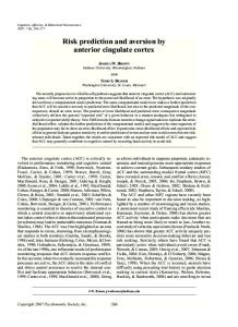
discount factor Fig. 1. The optimal intervals as a function of β. The thick, black lines show the optimal intervals on (the logarithm of) the ratio marginal utilities for the utility function lnðcÞ (as in Ligon et al., 2002), and the thin, blue (lighter) lines for c1 " σ =ð1 " σÞ with σ¼ 1.5. The dots represent βn . (For interpretation of the references to color in this figure caption, the reader is referred to the web version of this paper.)

The thick, black lines in Fig. 1 reproduce Fig. 1 in Ligon et al. (2002). The dashed lines represent the optimal intervals on the logarithm of x for the symmetric states, hh and ll (the two coincide with logarithmic utility), while the solid lines are the intervals for the asymmetric states, as a function of β. The thin, blue (lighter) lines in Fig. 1 show the corresponding intervals when σ ¼1.5, that is, when agents are more risk averse. First of all, notice that the intervals bounded by the thin, blue (lighter) lines are wider for all β. Let us look at the case where β ¼0.94 first. For this discount factor, all the intervals overlap, except the ones for states hl and lh (see the intervals along the vertical, dotted line in Fig. 1). In this case, the ratio of marginal utilities, after a sufficient number of periods, will only take two values, x hl and x lh ¼ 1=x hl , with probability 1. For the utility function uðÞ, these numbers are 0.940 and 1.064.12 When agents' preferences are described by the more concave function vðÞ, they equal 0.990 and 1.010,13 thus the optimal intervals are wider. It follows that the insurance transfers in the asymmetric states, hl and lh, are 4.53 and 4.92, for the utility functions uðÞ and vðÞ, respectively. This also means that if agents are more risk averse, consumption is smoother across states, so agents achieve more risk sharing. The coefficient of variation of consumption is 0.115 and 0.112 for the utility functions uðÞ and vðÞ, respectively. Consider β ¼0.9 as another example. In this case the coefficient of variation of consumption is 0.130 and 0.118, respectively. Hence, wider intervals imply less consumption variation, and in turn risk sharing as measured by one minus the ratio of consumption variation and income variation increases. n In Fig. 1 the dots represent the discount factor above which perfect risk sharing is self-enforcing, β . The black dot n n represents β ¼ 0:964 for the utility function uðÞ, while the blue (lighter) dot is at β ¼ 0:943, which belongs to the more concave utility function vðÞ. Notice that, as the dot moves to the left, the optimal intervals also move to the left, i.e. they become wider. Thus, we may capture the changes in the intervals, and thereby the changes in the transfers and the variation n of consumption, by the scalar β . Finally, let us consider the remaining measures of risk sharing. One can also compute Lucas and Robert's (1987) measure for any β. For example, for β ¼0.94 the proportional upward shift in the consumption process in autarky to make the agents just as well off as being in the risk-sharing arrangement is 1.010 and 1.018 for the utility functions uðÞ and vðÞ, respectively, nn while for β ¼0.9 it is 1.007 and 1.017, respectively. Finally, it is clear from Fig. 1 that β is lower when agents are more risk n reverse. Therefore, all these measures co-move with β in the right direction in this example. 5. Conclusion In a framework of mutual insurance subject to limited commitment, non-trivial conditions are required for more risk or higher risk aversion to relax participation constraints and allow more risk sharing. Even when agents face no aggregate risk, but their endowment may take more than three values, a mean-preserving spread that affects the support of the endowment distribution may destroy the sustainability of perfect risk sharing with voluntary transfers. When agents face aggregate risk, the same can happen even with only two possible endowment realizations. However, as long as aggregate risk is small and the minimum and maximum endowment levels do not change (i.e., when the increase in risk is not strong in the sense of Meyer and Ormiston, 1985), risk vulnerability as defined by Gollier and Pratt (1996) is sufficient to guarantee 12 13

The relevant optimal intervals are [0.5,0.940] and [1.064,2]. The relevant optimal intervals are [0.35,0.990] and [1.010,2.83].

S. Laczó / Journal of Economic Dynamics & Control 46 (2014) 237–251

251

the intuitive comparative statics result. In terms of risk aversion, in the presence of aggregate risk the intuitive comparative statics result holds only under very strong assumptions. These results point out that whether agents are able to share risk efficiently by mutual insurance subject to limited commitment can be affected in a counterintuitive way by policies that affect agents' risk attitudes towards their income, e.g. lump-sum transfers or social insurance, or change after-tax income risk, e.g. by changing the progressivity of the income tax system (Krueger and Perri, 2011), under general conditions. Acknowledgments This paper is based on a chapter of my doctoral thesis at the Toulouse School of Economics. I also benefitted from the hospitality of the European University Institute and the University of California, Los Angeles, while advancing this project. I thank an anonymous referee, Árpád Ábrahám, Pierre Dubois, Johannes Gierlinger, Christian Gollier, Bruno Jullien, Gergely Lakos, Thierry Magnac, Maurizio Mazzocco, Markus Reisinger, Raffaele Rossi, François Salanié, Karl Schlag, and participants of the Risk Sharing workshop in Toulouse, the Summer workshop at the Economic Institute, Hungarian Academy of Sciences in Budapest, ESEM in Milan, the ASSET meeting in Florence, the LERNA workshop in Toulouse, and EGRIE in Bergen for useful comments and suggestions. All errors are mine. Generous funding from Agence Nationale de la Recherche (ANR-06-BLAN0104) is gratefully acknowledged. Appendix A. Supplementary material Supplementary data associated with this article can be found in the online version at http://dx.doi.org/10.1016/j.jedc. 2014.06.013.

References Abreu, D., 1988. On the theory of infinitely repeated games with discounting. Econometrica 56 (2), 383–396. Alvarez, F., Jermann, U.J., 2000. Efficiency, equilibrium, and asset pricing with risk of default. Econometrica 68 (4), 775–797. Arrow, K., 1965. Aspects of the Theory of Risk-Bearing. Yrjo Jahnssonin Saatio, Helsinki. Attanasio, O., Ríos-Rull, J.-V., 2000. Consumption smoothing in island economies: can public insurance reduce welfare?. Eur. Econ. Rev. 44 (7), 1225–1258. Borch, K., 1962. Equilibrium in a reinsurance market. Econometrica 30 (3), 424–444. Broer, T., 2011. Crowding out and crowding in: when does redistribution improve risk-sharing in limited commitment economies?. J. Econ. Theory 146 (3), 957–975. Coate, S., Ravallion, M., 1993. Reciprocity without commitment: characterisations and performance of informal risk-sharing arrangements. J. Dev. Econ. 40, 1–24. Dixit, A., Grossman, G.M., Gul, F., 2000. The dynamics of political compromise. J. Polit. Econ. 108 (3), 531–568. Fafchamps, M., 1999. Risk sharing and quasi-credit. J. Int. Trade Econ. Dev. 8 (3), 257–278. Genicot, G., 2006. Does Wealth Inequality Help Informal Insurance?. Mimeo. Gollier, C., 2001. The Economics of Risk and Time. MIT Press, Cambridge, MA. Gollier, C., Pratt, J.W., 1996. Risk vulnerability and the tempering effect of background risk. Econometrica 64 (5), 1109–1123. Hadar, J., Russell, W.R., 1969. Rules for ordering uncertain prospects. Am. Econ. Rev. 59 (1), 25–34. Jewitt, I., 1987. Risk aversion and the choice between risky prospects: the preservation of comparative statics results. Rev. Econ. Stud. 54 (1), 73–85. Jewitt, I., 1989. Choosing between risky prospects: the characterization of comparative statics results, and location independent risk. Manag. Sci. 35 (1), 60–70. Kehoe, P.J., Perri, F., 2002. International business cycles with endogenous incomplete markets. Econometrica 70 (3), 907–928. Kimball, M.S., 1988. Farmers' cooperatives as behavior toward risk. Am. Econ. Rev. 78 (1), 224–232. Kocherlakota, N.R., 1996. Implications of efficient risk sharing without commitment. Rev. Econ. Stud. 63 (4), 595–609. Krueger, D., Perri, F., 2006. Does income inequality lead to consumption inequality? Evidence and theory. Rev. Econ. Stud. 73 (1), 163–193. Krueger, D., Perri, F., 2011. Public versus private risk sharing. J. Econ. Theory 146 (3), 920–956. Ligon, E., Thomas, J.P., Worrall, T., 2002. Informal insurance arrangements with limited commitment: theory and evidence from village economies. Rev. Econ. Stud. 69 (1), 209–244. Lucas, Robert E., J., 1987. Models of Business Cycles. Yrjo Jahnsson Lecture Series, Helsinki, Finland. Blackwell, London. Marcet, A., Marimon, R., 2011. Recursive Contracts, Mimeo. Mazzocco, M., 2007. Household intertemporal behavior: a collective characterization and a test of commitment. Rev. Econ. Stud. 74 (3), 857–895. Meyer, J., Ormiston, M.B., 1985. Strong increases in risk and their comparative statics. Int. Econ. Rev. 26 (2), 425–437. Pratt, J.W., 1964. Risk aversion in the small and in the large. Econometrica 32 (1/2), 122–136. Ross, S.A., 1981. Some stronger measures of risk aversion in the small and the large with applications. Econometrica 49 (3), 621–638. Rothschild, M., Stiglitz, J.E., 1970. Increasing risk: I. A definition. J. Econ. Theory 2 (3), 225–243. Schechter, L., 2007. Theft, gift-giving, and trustworthiness: honesty is its own reward in rural paraguay. Am. Econ. Rev. 97 (5), 1560–1582. Thomas, J., Worrall, T., 1988. Self-enforcing wage contracts. Rev. Econ. Stud. 55 (4), 541–554. Wilson, R., 1968. The theory of syndicates. Econometrica 36 (1), 119–132.