DOA Estimation Using MUSIC Algorithm for Quantized Data Project done under Summer Research Fellowship Program conducted by Indian academy of Sciences.
MAYUR AGRAWAL under the guidance of Professor G.V. Anand July 2005 Department of Electrical Communication Engineering Indian Institute of Science Bangalore 560 012
Acknowledgements Firstly, I would like to express my deepest sense of gratitude to Professor G. V. Anand for giving me the opportunity to work in his Lab. He was always there to provide the insightful thinking needed for completion of the Project. He has been a constant source of inspiration. I am also greatly indebted to Indian Academy of Sciences for selecting me for this program. It has really been an enriching experience for me. I would like to thank Saurabh for the innumerable discussions I had with him during my stay in Bangalore. Thanks are also due to my Lab mates— Rohit, Aditya, Pramod & Lalitha, for making my stay there a memorable one. They were real fun to work with.
Abstract Application of Optimal Quantization for direction-of-arrival (DOA) estimation using the popular MUSIC algorithm, one of the subspacebased algorithms, is presented. The effect of Quantization on mean square error (MSE) with variation in Generalized Gaussian index p, signal-to-noise-ratio (SNR) and bandwidth of the signal is investigated. The performance of MUSIC algorithm in the presence of phase errors in the array elements is analyzed. It is shown that for low SNRs, quantized data gives better results in comparison to unquantized data for certain probability density functions. The analysis assumes the array elements to be omnidirectional with unity gain. The noise model considered is both spatially and temporally white. Keywords—DOA estimation, eigenstructure methods, MUSIC, Stochastic Resonance, perturbation.
Contents 1 The 1.1 1.2 1.3
Data Model and MUSIC Signal Model . . . . . . . . . . . . . . . . . . . . . . . . . . . Noise Model . . . . . . . . . . . . . . . . . . . . . . . . . . . . Plane Wave DOA estimation using MUSIC . . . . . . . . . .
1 1 2 3
2 Optimal Quantization 2.1 Stochastic Resonance . . . . . . . . . . . . . . . . . . . . . . . 2.2 Symmetric 3-level Quantizer . . . . . . . . . . . . . . . . . . .
6 6 7
3 Perturbation of the Array
10
4 Simulation Results
10
5 Conclusions
12
Conventions and Abbreviations A e A a(θ) E[·] fo I i.i.d. k L M MSE MUSIC N p PM U (θ) pdf R S s(n) SR SNR U ULA w(n) x(n) β ν2 (·)T (·)H
LxM matrix, with its column being the steering vectors. Steering vector matrix of the perturbed array. Steering vector associated with the direction θ. Expectation operator. Center frequency. Identity matrix. identically & independently distributed. wave number of the incoming plane wave. Number of elements in an array. Number of directional sources. Mean Square Error. MUltiple SIgnal Classification. number of snapshots. Generalized Gaussian index. MUSIC Ambiguity function. Probability density function. Array correlation matrix. Source correlation matrix. Vector of source signals at nth snapshot. Stochastic Resonance. Signal-to-noise-ratio. Matrix with L eigen column vectors corresponding to eigenvalues of R. Uniform Linear Array. Noise vector at nth snapshot. Array signal vector at nth snapshot. Correlation decay parameter. Variance of i.i.d. Gaussian random variables with 0 mean. Transpose of a vector or matrix. Complex conjugate transpose of a vector or matrix.
Introduction This Report is concerned with the application of Optimal Quantization using Stochastic Resonance (SR) for improving the performance of array processors used for DOA estimation of plane waves. The performance of all DOA estimation techniques suffer rapid performance degradation when the SNR dips below 0 dB. This degradation however can be arrested by the use of Quantization as a preprocessing technique. Our primary interest is in DOA estimation for acoustic signals that emanate from submarines. In this Report we demonstrate the application of Quantization for DOA estimation of such signal using MUSIC algorithm. The initial sections of this Report are devoted for developing an appropriate model for our analysis.
1 1.1
The Data Model and MUSIC Signal Model
In a time varying medium such as ocean, it is often more appropriate to consider the signal to be a slowly and randomly modulated sinusoid. In other words, the signal is a sample function of a narrowband random process. The randomness in the signal can be attributed to the fluctuations of the source and the channel. The signal model in our case can be described as s(t) = a(t) cos(2πfo t) + b(t) sin(2πfo t)
(1)
where fo is the center frequency. The amplitudes a(t) and b(t) are zero mean independent Gaussian random processes with identical exponentially decaying autocorrelation functions E[a(t)a(t − k)] = σ 2 e−β|k|
(2)
2 −β|k|
(3)
E[b(t)b(t − k)] = σ e Also,
E[a(t)b(t − k)] = 0
(4)
where σ 2 is the variance of the signal in (1) and β is a measure of the bandwidth of the signal. Generally, this kind of random amplitude modulation occurs in media that introduce fading. We can characterize some of the statistical properties of the signal as follows: E[s(t)] = E[a(t) cos(2πfo t) + b(t) sin(2πfo t)] = E[a(t)] cos(2πfo t) + E[b(t)] sin(2πfo t)] = 0
(5) 1
E[s(t)s(t − k)] = E[{a(t) cos(2πfo t) + b(t) sin(2πfo t)} · {(a(t − k) cos(2πfo (t − k)) + b(t − k) sin(2πfo (t − k))}] = E[a(t)a(t − k)] cos(2πfo t) cos(2πfo (t − k)) + E[b(t)b(t − k)] sin(2πfo t) sin(2πfo (t − k)) = σ 2 e−β|k| cos(2πfo k)
(6)
The expression obtained above for the autocorrelation function of the signal shows that it is an exponentially decaying sinusoid.
1.2
Noise Model
It is a well known fact that in most marine environments the noise encountered is non-Gaussian. Hence we approximate the Generalized Gaussian distribution class as a model for non-Gaussian noise in our estimation problem. The Generalized Gaussian Family has the following density relation f (x, p , σ) =
p ς(σ, p) exp {− (ς(σ, p)|x|)p } 2 Γ(1/p)
(7)
where p > 0, is a positive parameter that controls the distribution0 s exponential rate of decay σ 2 is the variance of the distribution Γ(.) is the gamma function, given by Γ(n) =
Z ∞ 0
e−x xn−1 dx
ς(σ, p) is a scaling function of σ and p ,defined as ς(σ, p) =
1 σ
µ
Γ(3/p) Γ(1/p)
¶1/2
This Generalized Gaussian Family can encompass a wide variety of distributions, e.g., For p = 1, we get the Laplacian pdf ς(σ, 1) exp {−ς(σ, 1)|x|} 2 For p = 2, we get the Gaussian pdf f (x, 1, σ) =
f (x, 2, σ) =
n o ς(σ, 2) √ exp − (ς(σ, 2)|x|)2 π
(8)
(9)
As p → ∞, we get the uniform density function f (x, ∞, σ) =
ς(σ, ∞) ; 2
·
x∈
−1 1 , ς ς
¸
(10)
While as p → 0, we get an impulse probability function. Figure 1 plots some members of the family as a function of p. 2
3 p=0.5
2.5
f ( x, p, 1 )
2
1.5
1 p=1
0.5 p=3 p=20
0 −4
−3
−2
−1
0
1
2
x
3
4
xx
Figure 1: Variation of Generalized Gaussian probability density function f (x, p, σ) with x for p = 0.5, 1, 3, 20 & σ = 1.
1.3
Plane Wave DOA estimation using MUSIC
The model discussed here [1] is applicable for narrowband DOA estimation problem in case of unperturbed data. For simplicity our discussion is confined to the single parameter per source case (e.g. azimuth angle) only. However, the analysis presented can be easily extended to the multiple parameter case. Let us consider M radiating narrowband sources with center frequency fo observed by a ULA of L sensors with intersensor spacing d. Let x(n) denote the L x 1 vector of the signals at the array element outputs at the nth snapshot. A snapshot consists of a collection of J samples of data over the time j = 1, . . . J at each sensor. The array signal vector x(n) is obtained by taking the Fourier Transform over the J samples at each sensor and then selecting the appropriate frequency bin corresponding to the center frequency. Before proceeding further we enumerate the assumptions made in our problem formulation: 1. The sensors and sources are assumed to be coplanar with the number of sources M being less than the number of sensors L. 2. The sources are assumed to be far enough from the observing array so that the signal wavefronts are effectively planar over the array. 3. The DOA of the mth source is measured with respect to the end-fire 3
side of the array. The received signal vector can be written as x(n) = A s(n) + w(n)
(11)
where s(n) = [s1 (n) s2 (n) · · · sM (n)]T is the vector of the source signals at nth snapshot, and w(n) = [w1 (n) w2 (n) · · · wL (n)]T is the noise vector that is both temporally and spatially white. The steering vector matrix A is given by, A = [a(θ1 ) a(θ2 ) · · · a(θM )] (12) where h
a(θ) = 1 e−jkd cos θ
e−j2kd cos θ · · · e−j(L−1)kd cos θ
iT
.
(13)
The direction-finding problem can now be stated as follows: Given data M {x(n)}N n=1 estimate the unknown directions of arrival {θm }m=1 . The MUSIC Algorithm is based on the properties of the the covariance matrix of the vector of received signals. The covariance matrices of the signal and observation vectors are given by: S = E[s(n) s H (n)]
(14)
H
R = E[x(n) x (n)] 2 = A S AH + σw I
(15)
2 is the variance of the noise. where σw The eigenvalues of R can be divided into two sets [2] when the environment consists of uncorrelated directional sources and uncorrelated white noise. The eigenvalues in one set are all of equal values. Their value is independent of the directional sources and is equal to the variance of the white noise. The eigenvalues of second set are a function of the parameters of the directional sources with their number equal to the number of these sources. Each eigenvalue of this set is associated with a directional source, and its value changes with change in power of the source. The eigenvalues of this set correspond to the M largest eigenvalues of R. We refer to these eigenvalues as signal eigenvalues, and those corresponding to the first set as noise eigenvalues. Thus, the R of an array of L sensors immersed in M directional sources and white noise has M signal eigenvalues and L − M noise eigenvalues. Denoting the L eigenvalues of R in descending order by λl , l = 1, . . . L and their corresponding unit norm eigenvectors by U l , l = 1, . . . L, the matrix takes the following form:
R = UΛUH 4
(16)
where Λ = diag [λ1
λ2 · · · λL ] and U = [U 1
U 2 . . . U L] .
(17)
This representation is referred to as the spectral decomposition of R. The eigenvalues of R are orthogonal to each other and can be considered to span an L−dimensional space. This space can be divided into two orthogonal subspaces. The subspace spanned by signal eigenvectors is referred to as the ‘signal subspace’, whereas the subspace spanned by the noise eigenvectors is referred to as the ‘noise subspace’. The eigenstructure methods exploit the fact that the signal subspace is also spanned by M steering vectors associated with M directional sources. In principle, the eigenstructure based methods search for directions such that the steering vectors associated with these directions are orthogonal to the noise subspace and are contained in the signal subspace. In MUSIC we obtain the noise subspace by calculating an estimate of R from N data samples using b = R
N 1 X x(n) x H (n) N n=1
(18)
b Once the noise subspace has been followed by eigen decomposition of R. estimated, a search for M directions is made by looking for steering vectors that are as orthogonal to the noise subspace as possible. This is accomplished by searching for the M highest peaks of the function
PM U (θ) =
1 bwU b H a(θ) aH (θ) U w
(19)
b w are estimated eigen vectors corresponding to the where the columns of U noise subspace. Figure 2 shows a typical plot of Normalized Spectrum PM U (θ) as a function of θ.
Due to finite N , an error occurs in the estimation of R. This leads to an introduction of mean square error (MSE) in the DOA estimated using MUSIC. For a given N , the MSE of the MUSIC DOA estimator can be reduced by increasing the SNR. It will be illustrated in the section 4 that at low SNRs, estimation of θ by this algorithm degrades appreciably for unquantized data. The following section explores the possibility of Optimal Quantization as a preprocessing tool to obtain better DOA estimates at low SNRs.
5
1
(θ) )
0.7
MU
0.8
Normalized spectrum ( P
0.9
0.6 0.5 0.4 0.3 0.2 0.1 0 25
30
35
40
45
Direction of Arrival ( θ )
50
55
60
Figure 2: Variation of the Normalized Spectrum PM U (θ) as a function of the direction of arrival θ for 2 uncorrelated sources placed at θ1 = 40◦ , θ2 = 45◦ .
2 2.1
Optimal Quantization Stochastic Resonance
Stochastic Resonance (SR) is the phenomenon of enhancement of signal transmission by certain nonlinear systems resulting from the addition of noise to the system. In other words, a system driven by a periodic signal and stationary white noise, is said to exhibit SR, if at the output of the system, the SNR displays a non-monotonic behaviour with increasing input noise variance resulting in a peak value of SNR at a certain value of the input noise variance. In the field of DOA estimation, any non-linear system used for Quantization may be optimized using the phenomenon. With an apriori knowledge of noise statistics, the parameters of the system, in our case threshold, may be adjusted to improve its performance. Our Quantization model is based on the phenomenon of SR. As our primary interest in applying Optimal Quantization is for the estimation problem, we will skip the mathematical details and justifications needed to arrive at the expressions. However interested readers may refer to Guha [3] for a more comprehensive treatment on the subject.
6
2.2
Symmetric 3-level Quantizer
We consider a symmetric 3-level quantizer with threshold γ1 and quantization levels −1, 0 and 1 . If the quantizer is driven by a sequence x(n), then the output sequence y(n) is given by the relation −1
y(n) =
for x(n) ≤ −γ1 0 for − γ1 < x(n) ≤ γ1 1 for x(n) > γ1
(20)
Let the input x(n) be given by µ
2πn x(n) = ε1 cos − ϕ + σw(n), N
(21)
where w(n) are zero mean, unit variance i.i.d. random variables with pdf f (ζ) and probability distribution function F (ζ) : F (ζ) = P (w(n) ≤ ζ) ∀n dF (ζ) f (ζ) = dζ
(22) (23)
The probability distribution of the output y(n) is therefore given by P (y(n) = −1) = P (x(n) ≤ −γ1 )
= P w(n) ≤
³
−γ1 − ε1 cos
2πn N
σ
−ϕ
´
= F (−γ − εcn ) P (y(n) = 0) = P (−γ1 < x(n) ≤ γ1 )
(24)
= F (γ − εcn ) − F (−γ − εcn ) P (y(n) = 1) = P (x(n) > γ1 ) = 1 − F (γ − εcn ), where
ε=
ε1 σ
,
γ=
γ1 σ
³
,
cn = cos
2πn N
´
−ϕ .
It follows that the mean & variance of y(n) are given by: E[y(n)] = 1 − F (γ − εcn ) σy2 (n)
(25)
= var(y(n)) = 1 − F (γ − εcn ) + F (−γ − εcn ) − E[y(n)]2
(26)
Before proceeding further, we make the following assumptions: 1. The signal amplitude ε1 is considered very small compared to the noise standard deviation σ, i.e. ε = ε1 /σ ¿ 1 7
2. The noise pdf f (ζ) is assumed to be a symmetric function implying F (−ζ) = 1 − F (ζ). Under the above assumptions, we get E[y(n)] = F (γ + εcn ) − F (γ − εcn ) σy2 (n)
(27) 2
= 2 − F (γ + εcn ) − F (γ − εcn ) − E[y(n)]
(28)
Expanding F (γ + εcn ) and F (γ − εcn ) about γ using Taylor series, equations (27) and (28) can be written as µ
2πn − ϕ + O(ε3 ) N σy2 (n) = 2[1 − F (γ)] + O(ε2 ).
(29)
E[y(n)] = 2εf (γ) cos
(30)
Using the weak signal approximation and the expression for SNR gain (G) [3], we get 2f 2 (γ) G= (31) 1 − F (γ) It is seen from (31) that the gain depends on the input noise distribution and the parameter γ. Our interest is in determining the value of γ for which 10 9 8
SNR Gain (G)
7
p=0.5
6 5 p=20 4 3 2 1 0 0
p=1
p=3 0.5
1
1.5
2
2.5
3
Normalized Threshold (γ)
Figure 3: Variation of SNR gain of symmetric 3-level Quantizer as a function of the Normalized Threshold. The input noise pdf is Generalized Gaussian, with p = 0.5, 1, 3, 20.
8
2 1.8
Optimum Threshold ( γo )
1.6 1.4 1.2 1 0.8 0.6 0.4 0.2 0 0
2
4
6
8
10
12
14
16
18
20
Generalized Gaussian Index ( p )
Figure 4: Variation of the Optimal Threshold of symmetric 3-level Quantizer as a function of the Generalized Gaussian index p. G is at its maximum value. This optimal value γo , is obtained by equating dG dγ to zero. Hence γo is the positive root of the equation: 2[1 − F (γ)]
d f (γ) + f 2 (γ) = 0 dγ
(32)
If the above equation has no positive root, G is maximum at γ = 0. Figure 3 shows plots of G vs γ for different values of the Generalized Gaussian index(p). For p > 1, there exists an optimal value of γo satisfying (32). However for p ≤ 1, G is maximum at γ = 0. Hence the Optimal 3-level Quantizer has the degenerate form (
y(n) =
−1 for x(n) ≤ 0 1 for x(n) > 0
(33)
It is observed √ from Figure 4 that for p > 1, γo asymptotically approaches the value 3 as p → ∞. A comparison has been made between the MSE for quantized & unquantized data in section 4. The simulation results would clearly demonstrate a reduction in MSE at low SNR for quantized data. The next section deals with the perturbation of the array.
9
3
Perturbation of the Array
The data model developed in Section 1 required certain modeling assumptions to be made. It was assumed that the array response in all directions of interest and the spatial covariance of the noise are known exactly. In practice, however, neither of these quantities is known precisely. Depending on the degree to which they deviate from their normal values, serious performance degradation may result. Significant work [4] has been done to study the effects of perturbation on the performance of MUSIC for DOA estimation. We will limit our discussion to the phase perturbation associated with the array. Based on the model suggested by Swindlehurst and Kailath [4], the steering vector matrix of the perturbed array can be written as e = ΓA , A h
Γ = diag ejξ1 ξi =
i X
αk ,
ejξ2 · · · ejξL
i = 1, 2, · · · L
(34)
i
,
(35) (36)
k=1
where α1 , α2 , · · · αL are i.i.d. Gaussian random variables with mean zero and variance ν 2 . Accordingly, our data model (11) changes to e s(n) + w(n) x ˜ (n) = A
(37)
where x ˜ (n) is the L x 1 data vector at the nth snapshot. We performed our next set of simulations with the modified model developed. The results are shown in the next section.
4
Simulation Results
In all the simulations performed, the sources were assumed to be uncorrelated narrowband signals of same power with the same center frequency fo . Unless otherwise specified, the bandwidth of all the signals was taken to be same with β = 0.005. The signal was sampled at 8 times the center frequency with a snapshot consisting of 16 samples of data over time. A ULA with intersensor spacing d = λ/2 was considered all throughout to avoid spatial aliasing. The Generalized Gaussian noise added to the signal at every sensor was assumed to be both spatially & temporally white with variance 2 = 1. The desired input SNR was obtained by varying σ in (2), (3). σw The simulations for array perturbations were performed by adding uncorrelated zero mean Gaussian random phases to the array signals as specified by (34), (35), (36). The Bias and MSE were calculated by averaging over 500 Monte Carlo Simulations. 10
0.045
Mean Square Error (MSE)
0.04 0.035 0.03 0.025 0.02 0.015 0.01 0.005 0 10
20
30
40
50
60
70
80
Direction of Arrival (θ)
Figure 5: Variation of MSE as a function of θ for a single source with SNR= 0 dB, p = 0.5, N = 128, L = 12, β = 0.005. Figure 5 shows the dependence of MSE on DOA in degrees for unquantized data. It is observed that as we move towards the broadside of the array the error incurred in estimation decreases, which is along expected lines. This is due to the fact that the spatial frequency of the incoming signal decreases, even though the spatial sampling frequency remains the same. This results in a better sampling of the signal, hence the MSE progressively goes down for our movement from fire end side to broadside of the array. In Figure 6, we demonstrate the better performance of quantized data over unquantized data for low SNRs. It is seen that for SNRs less than about −8 dB, the MSE error for quantized data is substantially lower than that for unquantized data. We also observed a better resolving power in case of quantized data. We had considered 2 directional sources at an angular separation of 10◦ for our analysis with p = 0.5. Figure 7 compares the variation of MSE with p for SNR= −15 dB. It is observed that the unquantized data gives better performance only in the range p ∈ [1.5, 4]. We conclude that as the departure of the noise pdf increases from Gaussian (p = 2), quantization yields better & better results. The results presented in Figure 8, 9 illustrate the variation of MSE with β. For SNR= 0 dB, unquantized data gives better results, but for SNR= −15 dB, it is the quantized data which gives superior results. We also observe that MSE increases with increase in bandwidth of the signal. As the bandwidth increases, our assumption of narrowband signal approximation 11
becomes weaker. This results in increase in MSE. One interesting point to observe is that for very low value of β, MSE increases with decrease in β. So far our analysis has been limited to the unperturbed case with ν 2 = 0. We give now the results for the perturbed case in Figure 10, 11. It is again observed that quantized data outperforms unquantized data for SNR= −16 dB. However at 10 dB, it is again the unquantized data which gives better results.
5
Conclusions
We have presented in this Report a better method to estimate DOA using MUSIC for low SNRs. We developed our model for Optimal Quantization using Stochastic Resonance. It was shown that quantized data outperforms unquantized data for a large number of probability density functions that are non-Gaussian. Simulation results were presented to demonstrate the validity of our claim and the advantage of Optimal Quantization. The performance of quantized data in the presence of perturbation was also analyzed. The analysis was limited to the case of phase perturbation in the array. We were again able to demonstrate the usefulness of Quantization. It would be worthwhile to look back at our results obtained in Figure 8, 9. We were unable to find suitable reason for high MSE incurred in the estimation of θ at very low β. It would be interesting to investigate this further.
12
7 Unquantized Quantized
Mean Square Error (MSE)
6
5
4
3
2
1
0 −20
−15
−10
−5
0
5
10
SNR ( in dB)
Figure 6: Variation of MSE as a function of SNR for Quantized & Unquantized Data with p = 0.5, N = 128, L = 12, β = 0.005.
0.1 Quantized Unquantized
Mean Square Error (MSE)
0.09 0.08 0.07 0.06 0.05 0.04 0.03 0.02 0.01 0
2
4
6
8
10
12
14
16
18
20
Generalized Gaussian index (p)
Figure 7: Variation of MSE as a function of p for Quantized & Unquantized Data with SNR= −15 dB, N = 256, L = 12, β = 0.005.
13
0.05 Unquantized Quantized
0.045
Mean Square Error (MSE)
0.04 0.035 0.03 0.025 0.02 0.015 0.01 0.005 0 −4 10
−3
−2
10
−1
10
10
Correlation Decay Parameter (β)
Figure 8: Variation of MSE as a function of β for Quantized & Unquantized Data with SNR= 0 dB, p = 0.5, N = 128, L = 12.
1 Quantized Unquantized
0.9
Mean Square Error (MSE)
0.8 0.7 0.6 0.5 0.4 0.3 0.2 0.1 0 −4 10
−3
−2
10
10
−1
10
Correlaton Decay Parameter (β)
Figure 9: Variation of MSE as a function of β for Quantized & Unquantized Data with SNR= −15 dB, p = 0.5, N = 128, L = 12.
14
1 Unquantized Quantized
0.9
Mean Square (MSE)
0.8 0.7 0.6 0.5 0.4 0.3 0.2 0.1 0
−4
−3
10
10
−2
10
ν2
Figure 10: Variation of MSE as a function of ν 2 for Quantized & Unquantized Data with SNR= 10 dB, p = 0.5, M = 1, N = 128, L = 12. 1 Unquantized Data Quantized Data
0.9
Mean Square Error (MSE)
0.8 0.7 0.6 0.5 0.4 0.3 0.2 0.1 0
−4
−3
10
2
ν
10
−2
10
Figure 11: Variation of MSE as a function of ν 2 for Quantized & Unquantized Data with SNR= −16 dB, p = 0.5, M = 1, N = 128, L = 12. 15
References [1] B. Friedlander, “A Sensitivity Analysis of the MUSIC Algorithm”, IEEE Trans. ASSP, vol. 38, pp. 1740-1751, October 1990. [2] L. C. Godara, “Application of Antenna Arrays to Mobile Communications, Part II: Beam-Forming and Direction-of-Arrival Considerations” Proc. IEEE, vol. 85, pp. 1195-1245, August 1997. [3] V. G. Guha, “Detection of weak signals in Non-Gaussian Noise using Stochastic Resonance”, August 2002. [4] A. L. Swindlehurst, “A Performance Analysis of Subspace-Based Methods in the Presence of Model Errors, Part I: The MUSIC Algorithm”, IEEE Trans. SP, vol. 40, pp. 1758-1773, July 1992.