Distributed Adaptive Bit-loading for Spectrum Optimization in Multi-user Multicarrier Systems ⋆ Sumanth Jagannathan and John M. Cioffi Department of Electrical Engineering, Stanford University, Stanford, CA 94305 {sumanthj, cioffi}@stanford.edu
Abstract This paper presents a low-complexity discrete bit-loading algorithm for multi-user multicarrier systems with application to spectrum balancing in digital-subscriberlines. The algorithm can be implemented in a distributed manner using limited information that is sent to modems by a spectrum management center (SMC). The SMC classifies users in the network as strong or weak, based on their channel and noise conditions. Weak users execute a discrete bit-loading algorithm approximating water-filling, such as the Levin-Campello (LC) algorithm, while strong users use a rate-penalty table along with a modified LC algorithm to limit their interference to weak users. Simulation results show that the proposed algorithm can achieve nearoptimal performance. In addition, polite bit and gain adaptation algorithms are developed using the structure of the proposed bit-loading algorithm, which enables easy and fast adaptation to channel and noise variations. Key words: Digital-subscriber-lines (DSL), Dynamic spectrum management (DSM), Multicarrier, Interference channel, Spectrum optimization
1
Introduction
1.1 Background and Motivation Optimization of the transmit spectra among multiple users is an important consideration in modern communication systems. With a limited bandwidth ⋆ This work was supported by the NSF under contract CNS-0427711 and France T´el´ecom R&D.
Preprint submitted to Elsevier
April 24, 2008
and an increasing number of users, the achievable data rates in various wireless and wireline networks are being limited by the interference between users. One example is the digital-subscriber-line (DSL) network where users transmit over copper twisted-pairs or quads that share the same binder/cable. The electromagnetic interference between the copper lines (usually referred to as crosstalk) becomes a severe limitation to the data rate when the distance between the interfering transmitter and the victim receiver is small. Therefore, careful management of the crosstalk between the various users sharing a cable is important to provide high data rates to more users or to reduce the power consumption in the network, which is gaining importance in the telecommunications industry [1][2]. Dynamic Spectrum Management (DSM) [3][4] provides a framework for such management; specifically, level-2 DSM methods, often referred to as spectrum balancing algorithms, optimize the users’ spectra by considering the harm caused to each other by crosstalk. Essentially, in level-2 DSM, transmission by users in the network is modeled as communication over a frequency-selective interference channel with the interference between users treated as noise. Such an approach provides significant gains over current level-0 and level-1 DSM systems, which try to optimize the DSL parameters (power, margin, spectrum, etc.) of each line from a single-user perspective without considering the harm caused to other users in the network. Level-2 DSM methods also have a role to play in future level-3 DSM systems (also called vectored systems), where users are coordinated at the signal-level at either the transmitter or receiver to cancel the crosstalk between them. However, practical constraints, such as the complexity of the equipment, may prevent complete cancellation of crosstalk between all 100 lines of a cable in the near future. Therefore, a good intermediate solution would be to form smaller groups of lines; the crosstalk within each vectored group can be canceled, while the interference between the different vectored groups can be managed using a spectrum balancing algorithm. In view of the various benefits of level-2 DSM, it is important to develop practical algorithms for spectrum balancing.
1.2 Previous Work on Spectrum Balancing
One of the early spectrum balancing algorithms in DSM is the iterative waterfilling (IWF) algorithm [5], which obtains significantly higher data rates than currently-used static spectrum management methods. IWF has a number of desirable features such as its distributed nature of implementation, lowcomplexity, and adaptability to changing channel and noise conditions. Moreover, it has a natural discrete bit-loading implementation based on existing algorithms that approximate single-user water-filling such as the LevinCampello (LC) algorithm [6][7]. A shortcoming of IWF is that it is sub2
optimal in near/far scenarios encountered in upstream VDSL (see Fig. 7) and central-office (CO)/remote-terminal (RT) mixed-binder downstream situations 1 . IWF is sometimes considered a level-1 DSM technique since it can be implemented without introducing new controls in current standards. However, improvements in the implementation of the bit and gain swapping procedures [3] as well as consideration of the limits in current standards on the PSD increment/reduction during online operation (referred to as SHOWTIME in DSL) are required to obtain the benefits of IWF. The optimal solution to the spectrum balancing problem based on Lagrange dual decomposition was provided by the optimal spectrum balancing (OSB) [8] algorithm. While the OSB algorithm has a linear complexity in the number of subchannels (or subcarriers), its exponential complexity in the number of users and its centralized nature make it prohibitive for practical implementation. Iterative spectrum balancing (ISB) [9][10] significantly reduces the complexity of OSB but is still centralized. Both the OSB and ISB algorithms work by either assuming discrete bit-loading or a discretization of the powerspectral-density (PSD) levels. Unlike OSB and ISB, a continuous bit-loading algorithm 2 called SCALE [11] was developed by applying a convex relaxation technique to the non-convex spectrum balancing problem. With SCALE as a starting point, the authors in [12] presented a greedy algorithm to generate a discrete bit-loading for use in practical systems. However, the SCALE algorithm requires real-time message passing between the various modems and the central spectrum management center (SMC) [4], thus limiting its practical implementation. In pursuit of a more distributed but near-optimal solution, the band preference methodology was proposed in [13] where modems independently perform water-filling based on the power-spectral-density (PSD) masks or water-level scaling factors [14][15] provided by the SMC. The intuition behind the bandpreference algorithms is that users should first try to use frequency bands where they create less crosstalk or bands that are not used by other users. If the required target data rate cannot be met, then bits can be loaded in the remaining subchannels in a polite manner. Autonomous Spectrum Balancing (ASB) [16] is another distributed algorithm where information about a typical “reference” line in the network is initially passed to the modems, which then independently perform their optimization. The modems try to achieve their target data rates while maximizing the data rate of the reference line. The hope then is that protecting the reference line will also help protect other lines in the network. 1
Refer to Fig. 2. A fiber-fed RT causes severe crosstalk to a user served by a CO, while the RT user does not experience much interference from the CO. 2 In discrete bit-loading, the number of bits on a subchannel is restricted to be an integer, while continuous bit-loading allows any non-negative real-valued bits.
3
Previous work on spectrum balancing has not considered adaptation to slow channel and/or noise variations by adjusting the bits and energies (or gains) of the subchannels 3 . However, such adaptation is very important since the users’ PSDs are optimized for a specific channel and noise situation during initialization, but the lines could experience variations in the noise spectra during online operation. Such variations could be caused by other DSLs in the binder turning on/off, changing temperature and soil conditions, or simply other non-crosstalk noise sources (TV, microwave, etc.) that vary with time. In the single-user case, the optimal LC discrete bit-loading algorithm allowed for easy adaptation [17]. Although the authors in [18][19] extended the LC algorithm to the multi-user case, the extension is centralized and is not amenable to bit and gain changes.
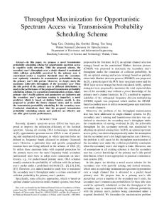
1.3 Summary of the Proposed Algorithm and Contributions This paper presents a discrete bit-loading algorithm for spectrum balancing, which achieves near-optimal performance in a distributed manner using limited information that is sent to modems by the SMC. Figure 1 provides an overview of the framework using which the spectrum balancing algorithm, which is referred to as spectrum-balancing-Levin-Campello (SBLC), is developed in this paper. Users in the network are classified as strong or weak by the SMC using knowledge of their channel transfer functions and noise spectra or by monitoring the users’ DSL parameters and performance. For example, in near-far situations, the near user will typically be classified as the strong user and the far user will be classified as the weak user. In CO/RT mixed-binder situations, the CO users will typically be the weak users and the RT users will be the strong users. In general, the SMC can perform the classification based on the actual network topology and channel/noise conditions. � � ��� � � � � � � � � � � �� � ���� � �� � � �� �� � �� �
� � � � �� � � � � � � �� � � � ��� � � � ��� �� � �� � � � � � � �� �! � " � � # � ��$ � � �� � � � � ���� !
� � %� �� � ��$ � � �� � � � � ��� � !
Figure 1. Framework for near-distributed spectrum balancing 3
Such adjustment is referred to as bit/gain-swapping in DSL.
4
After the classification of users, the modems of the weak users are directed to execute their normal bit-loading algorithm, which is usually a discretebit approximation of water-filling. On the other hand, the strong users are directed to execute a polite bit-loading algorithm, which causes minimal harm to the data-rate of the weak users. The SBLC algorithm uses a modified LC algorithm along with a rate-penalty table to reduce the amount of interference caused by strong users to weak users. The rate-penalty table represents the reduction in the data rate of the weak user when the strong user adds more bits to a subchannel. These tables can be formed by the modems using information about the weak user(s) sent by the SMC, or can be formed by the SMC and then sent to the modems with efficient compression. This paper presents a method to classify users as weak or strong, and to determine which user each strong user should protect. In general, each strong user can protect a different user in the network. The SBLC algorithm has lower complexity compared to other state-of-the-art discrete bit-loading algorithms for spectrum balancing and its complexity is close to that of IWF. While this paper describes a situation with one SMC, there could be multiple SMCs in an unbundled environment, one for each service provider. In such situations, the politeness enforced by one service provider’s SMC will also benefit the other service providers’ users. Moreover, regulatory requirements could play a role where the RT-users of all service providers are directed to protect the weaker CO users. For example, any RT-based DSL may be directed to protect a CO line of up to k kft where “k” is supplied by the service provider or regulator. The remainder of the paper is organized as follows. The system model and problem definition are described in Section 2. The incremental-energy and rate-penalty tables are introduced in Section 3. The SBLC algorithm is described Section 4, while the classification of users as weak/strong and the politeness mapping between strong users and the protected users are discussed in Section 5. Bit- and gain-adaptation procedures based on the SBLC algorithm are discussed in Section 6. The ASB algorithm for discrete bit-loading is described in Section 7 and the complexity of the various discrete bit-loading algorithms are analyzed in Section 8. A recent model for the crosstalk channels is briefly discussed in Section 9. Simulation results that show the performance of the bit-loading and adaptation algorithms are presented in Section 10. Finally, the paper is concluded in Section 11.
2
System Model and Problem Definition
A multi-user multicarrier system with N subchannels and U users is considered with one transmitter and receiver for each user. Assuming there is no 5
inter-carrier interference and that the users are synchronized, the channel can be modeled as N parallel and independent subchannels, each of which is an interference channel with U users. Such a model can be applied independently to the upstream and downstream of a DSL system that employs frequencydivision duplexing, or may be applied in a full-duplex DSL system by treating the upstream and downstream as separate interfering users. n On subchannel n, the direct channel of user u is denoted as Hu,u , while the n crosstalk channel from user v to user u is denoted as Hu,v . The background noise at user u’s receiver on subchannel n is assumed to be Gaussian with zero mean and energy (σun )2 . Denoting the energy transmitted by user v on subchannel n as Evn , the channel signal-to-interference-plus-noise ratio (SINR) of user u on subchannel n is expressed as n 2 |Hu,u | . n n 2 n 2 v6=u Ev |Hu,v | + (σu )
gun = P
(1)
Denoting the smallest incremental unit of information that can be transmitted as β bits (typically β = 1), the number of bits for user u on subchannel n can be expressed as $ �% � 1 Eun gun n bu = β , (2) log2 1 + β Γ where Γ is the product of the gap-to-capacity of the code [17] and the SINR margin used for protection against unexpected noise, and ⌊·⌋ denotes the rounding-down (floor) operation. The data rate for user u is then given by Ru =
N X
bnu .
(3)
n=1
The general goal of spectrum balancing is to allow weak users in the network to maximize their data rates, while strong users try to achieve their target data-rates while causing minimal interference to the weak users. Mathematical formulation of this problem is convenient when target data-rates are fixed for U − 1 users and the data rate of the U th user is to be maximized, i.e., maximize RU subject to Ru ≥ Rutarget , for u = 1, . . . , U − 1 Eu =
PN
n=1
Eun ≤ Eutot , ∀u
,
(4)
Eun ≤ Cun , ∀u, n bnu ≤ ¯b, ∀u, n
where for user u, Eutot is the total energy limit, Cun is the PSD mask constraint, and ¯b is the maximum bit-cap for each subchannel. A bit-cap, ¯bnu , that varies 6
among the users and subchannels can also be easily incorporated into the proposed algorithm. The development of the strong-user’s polite bit-loading algorithm in SBLC is motivated by a 2-user example with one weak and one strong user. In this case, the goal of spectrum balancing would be for the strong user to maximize the weak user’s data-rate while meeting its own target data-rate. This problem can also be thought of as the strong user trying to minimize the data-rate penalty that its crosstalk imposes upon the weak user. Section 4 essentially incorporates these data-rate penalties into the loading algorithm of the strong user to ensure politeness towards the weak user.
3
The Incremental-energy and Rate-penalty Tables
The SBLC algorithm employs a couple of tables for each user, which are used to determine the number of bits to be loaded on each subchannel in an incremental fashion. They are the incremental-energy table, which is used by both strong and weak users to determine the subchannel of least incrementalenergy cost where a bit can be loaded, and the rate-penalty table, which is used to determine the subchannel in which loading a bit by a strong user causes minimum penalty to the data-rate of the weaker user.
3.1 The Incremental-energy Table
To form the incremental-energy table, each user u’s receiver measures its channel SINR, gun , ∀n. Using (2), the minimum energy required for loading bnu bits, which is a multiple of β, on subchannel n is Eun (bnu ) =
� Γ � bnu 2 − 1 . gun
(5)
The incremental-energy required to transmit bnu bits on subchannel n for user u is then defined as
enu (bnu ) =
E n (bn ) − E n (bn − β) if bn > β u u u u u E n (bn ) u
=
u
if bnu = β
� Γ bnu � −β 2 1 − 2 . gun
(6)
7
Table 1 Incremental-energy Table for User u with β = 1
bnu
6
e1u (6)
∞
∞
···
∞
5
e1u (5)
∞
e3u (5)
···
∞
4
e1u (4)
e2u (4)
e3u (4)
···
∞
3
e1u (3)
e2u (3)
e3u (3)
···
∞
2
e1u (2)
e2u (2)
e3u (2)
···
eN u (2)
1
e1u (1)
e2u (1)
e3u (1)
···
eN u (1)
1
2
3
···
N
�� �
� ��
n
An incremental-energy table, such as Table 1, is formed by each user, which indicates the amount of energy required to load an extra β bits on subchannel n. When no more bits can be loaded on a subchannel because of violation of the PSD mask or bit-cap, the incremental-energy is set to ∞. Such an incremental-energy table is used in the optimal LC algorithms for single-user discrete bit-loading. While the gap to capacity is almost constant for many practical codes over a wide range of signal-to-noise-ratios (SNRs), there can be some deviation in practice based on the constellation size and type of code used. An advantage of the LC-based approach is that the incremental-energy table can be determined exactly by the modem based on the constellation and code that are used, instead of using the gap approximation [6].
3.2 The Rate-penalty Table
The second table used by strong users in the SBLC algorithm is a rate-penalty n table. For a strong user, u, the rate-penalty table Bpen,u (bnu ), indicates the reduction in bits for a weaker user when the strong user loads bnu bits on subchannel n. The table can be formed by choosing another user in the binder/cable that the strong user should protect, the determination of which is discussed in Section 5. Let user v be the weaker user that needs to be protected by strong user u. A nominal energy-allocation, Evnom,n , is assumed for user v, which could simply be its PSD mask or could be obtained by water-filling with the nominal background noise. Using Evnom,n , the penalty table is defined as 8
Table 2 Incremental Rate-penalty Table for user u with N = 10, β = 1 6
1
0
1
1
1
0
0
0
0
0
5
0
1
1
0
0
0
0
0
0
0
4
0
0
0
1
0
1
0
0
0
0
3
1
1
0
0
1
0
0
0
0
0
2
0
0
1
1
0
0
0
0
0
0
0
0
0
0
1
1
0
0
0
0
1
2
3
4
5
6
7
8
9
10
!%!
−
1 bnu
�� � n Bpen,u (bnu )
� ��
n
n 2 E nom,n |Hv,v | 1 = min ¯b, β log2 1 + v n 2 β Γ(σv )
$
1 min ¯b, β log2 1 +
β
�
n 2 Evnom,n |Hv,v |
n |2 + (σ n )2 Γ Eun (bnu )|Hv,u v
� ,
(7)
and the incremental rate-penalty table is defined as n Binc,u (bnu )
Bn
=
n pen,u (bu )
n − Bpen,u (bnu − β) if bnu > β
Bn
n pen,u (bu )
if bnu = β
(8)
for bnu = β, 2β, . . . , ¯b. The remainder of the paper assumes β = 1 without loss of generality. n Binc,u measures user v’s incremental loss of bits caused when strong user u loads an extra bit on subchannel n. Table 2 shows an example of an incremental rate-penalty table. The shaded regions will be explained later. The rate-penalty table can be computed by the strong user’s modem if the SMC provides it with information about the user that it needs to protect. This information would be the crosstalk channel from the strong user to the weaker user and the weaker user’s background noise spectrum, where both quantities are normalized by the product of the direct channel of the weaker user and its nominal PSD divided by the gap. Alternately, the SMC could compute the rate-penalty table and send it to the strong user’s modem. The information that needs to be sent to the modem can be reduced by efficiently compressing the rate-penalty table using techniques such as run-length coding [20] since the incremental rate-penalty table typically consists of a string of zeros followed by ones, especially when the crosstalk coupling is large. Moreover, one can think of approximations to obtain the table by passing an “equivalent length” parameter to the strong user’s modem, which provides it some idea of the ratio of it’s crosstalk channel to the direct channel of the weaker user, and assuming a background noise level for the weaker user.
9
4
The SBLC Algorithm
The fixed-margin (FM) and rate-adaptive (RA) LC algorithms form an important part of the SBLC algorithm and are discussed first. RA LC (Algorithm 1) maximizes the data rate of a single user subject to an energy constraint. In RA LC, the user greedily allocates a bit to the subchannel with the least incremental-energy cost at each iteration, and the procedure continues until the power, PSD, or bit-cap constraints become active. The FM version, which minimizes the energy subject to a target data rate, is obtained by replacing m the stopping criteria in Step 4 of the RA LC algorithm with em u (bu + 1) = ∞ target or Ru ≥ Ru . Algorithm 1 Rate-adaptive (RA) LC algorithm for user u 1: Initialization: Form the incremental-energy table enu , ∀n. Set Eun ← 0, bnu ← 0, ∀n. Therefore, Eu = 0 and Ru = 0. 2: loop 3: Set m ← arg minn enu (bnu + 1) m m m tot 4: if em u (bu + 1) = ∞ or (Eu + eu (bu + 1)) > Eu then 5: stop 6: else m m m 7: bm u ← bu + 1, Eu ← Eu + eu (bu ), Ru ← Ru + 1 8: end if 9: end loop In the SBLC algorithm, the weak users simply execute the FM LC algorithm if they are provided with a target data rate; otherwise, they execute the RA LC algorithm. Strong users will try to attain their data-rate target while causing minimum amount of penalty to the weaker users. The users execute their algorithms independently until their PSDs converge. If the SMC classifies all users to be weak, then the users effectively participate in an IWF procedure [5]. Next, the polite bit-loading algorithm, which is used by the strong users, is explained.
4.1 The Strong-user Algorithm
The algorithm executed by the strong user when implementing SBLC can be divided into 3 steps, which are listed below and are explained in the following subsections: (1) Perform bit-loading without causing any penalty to the weaker user. (2) If the target data-rate is not met, load the remaining bits while causing minimum penalty to the weaker user. 10
(3) Move bits from subchannels with higher incremental-energy costs to those with lower incremental-energy costs until the sum-energy constraint is satisfied. The PSD-mask and bit-cap constraints are implicitly satisfied when using the incremental-energy table to perform the bit-loading and don’t have to be considered explicitly during the bit-loading process. 4.1.1 Step (1): Initial Loading without Penalty Since the goal of the strong user is to cause minimum penalty to the weaker user, it first tries to achieve its target data-rate without causing any penalty to the weaker user. Therefore, the subchannels Nnp ⊆ {1, . . . , N } on which no rate-penalty is caused to the weaker user are chosen by identifying the n columns n of Binc,u that are all zeros. For example, columns 7 to 10 of Table 2 correspond to Nnp . The FM LC algorithm is executed on Nnp to try to achieve the target data-rate without causing any data-rate penalty to the weaker user. If the target data-rate is not met, then the remaining subchannels Np = {1, . . . , N }\Nnp become candidates for energy-allocation. However, even among Np , there could be some subchannels, such as subchannels 1 to 4 of Table 2, where the strong user could load a few bits without causing penalty to the weaker user. This often happens in low-frequency subchannels where the crosstalk coupling is weak and the background noise of the weak user dominates its performance as long as the crosstalk from the strong user is small. The polite loading on Np is achieved by executing the FM LC algorithm on these subchannels with a modified energy table e˜nu , where ∀n ∈ Np and b ∈ {1, . . . , ¯b}, e˜nu (b)
en (b) if B n u pen,u (b) = 0
=
∞
n if Bpen,u (b) 6= 0
.
(9)
Therefore, the first FM LC run using Nnp completely avoids overlapping the strong user’s PSD with that of the weaker user, while the second FM LC run using Np tries to achieve the target data-rate by loading on the overlapping subchannels but still without penalizing the weaker user. For example, the light-shaded cells in Table 2 show the bit-loading achieved by the two FM LC runs. If these two passes are not sufficient to meet the target data-rate, then the strong user has no option but to cause penalty to the weaker user, which is considered next. 4.1.2 Step (2): Loading with Minimum Penalty In the second step, the remaining bits required to meet the target data-rate of the strong user are loaded in subchannels Np while causing minimum penalty 11
to the weaker user. Let the bit-allocation for the strong user u obtained after Step (1) be denoted by ˜bnu , and let the final bit-allocation after Step (2) be denoted by ˆbnu . The problem of minimizing the rate-penalty caused to the weak user can be formulated as: N X
minimize subject to
n=1 N X
n Bpen,u (ˆbnu )
ˆbn = Rtarget , u u
n=1 ˆbn ≥ u
(10)
˜bn , ∀n u
where the constraints are that the target data-rate should be achieved and that the bit-allocation after Step (2) should be obtained by adding bits, and not removing them, starting with the bit-allocation obtained after Step (1). This problem can be alternately expressed as: minimize subject to
N X
ˆn
bu X
n Binc,u (b)
n=1 b=˜bn +1 u N X ˆbn = Rtarget u u n=1
,
(11)
4.1.2.1 Dynamic programming: The problem in (11) can be optimally solved using dynamic programming [21][15]. The cost function is defined as: ˜b1 +w1 u
J1 (w1 ) =
X
1 Binc,u (b)
(12)
b=˜b1u +1
+ln ˜bnuX
Jn (wn ) = min 0≤ln ≤wn
b=˜bn u +1
n Binc,u (b) + Jn−1 (wn − ln ) , n = 2, . . . , N,
(13)
where Jn (wn ) is the minimum cost to load wn extra bits on subchannel n. The optimal solution to the penalty minimization problem is then given by P ˜n JN (Rutarget − N n=1 bu ). The cost functions for n > 1 can be computed recursively, while J1 (w1 ) can directly determined using the incremental penalty P ˜n table. Therefore, the optimal penalty cost JN (Rutarget − N n=1 bu ) can be found at the end of the recursion along with the new bit-allocation, ˆbnu , which meets the data-rate target. Without loss of generality, the dynamic programming recursion can be executed only over the set of subchannels Np since the remaining subchannels would have already been loaded to the maximum possible extent in Step (1). 12
One might argue that Step (1) is not required since the penalty minimization problem in Step (2) would result in a minimum penalty for the weak user even if the initial bit-allocation were all zeros; therefore, Step (2) can be directly executed by skipping Step (1). However, the complexity of optimally solving the penalty minimization problem would be very high if all subchannels need to be considered in the dynamic programming recursion. Secondly, using Step (1) to initially avoid causing any penalty is a prudent approach since avoiding overlap of the strong and weak users’ PSDs will result in a more robust operating point for the network with respect to changes in the users’ channel or noise conditions. Moreover, a simpler algorithm can be used for Step (2) instead of the complex dynamic programming solution and this is described next.
4.1.2.2 Heuristic incremental approach: While dynamic programming can minimize the penalty caused to the weak user, it may be very complex to implement in practical modems. Moreover, the SHOWTIME adaptability of the strong-user’s bit-loading algorithm may suffer if such a complicated recursive subroutine is present in the algorithm. Therefore, an alternate heuristic method to load the remaining bits while trying to minimize the penalty is considered. In this approach, the subset of subchannels, Np,min ⊆ Np , having the minimum incremental rate-penalty after Step (1) is considered, i.e., n m ˜n Np,min = {m s.t. Binc,u (˜bm u + 1) = min Binc,u (bu + 1)}. n∈Np
(14)
For these subchannels, the number of bits, ∆b, that could be loaded before the next penalty is caused is computed. The subchannels with maximum ∆b ∆bmax , where the maximum value is ∆bmax . Essentially for are denoted by Np,min the same amount of penalty caused, subchannels where the maximum number of bits can be loaded by the strong user are selected as candidates (shown in dark shade in Table 2, where ∆bmax = 3). For these subchannels, the remaining n rate-penalty, Brem,u , that could be caused is calculated as bn max,u n Brem,u
=
X
n Binc,u (b),
(15)
b=˜bn u +1
where bnmax,u is the maximum number of bits that can be loaded on subchannel n by user u, which is determined by the PSD-mask and the bit-cap constraints. ∆bmax having the minimum remaining The subset of subchannels Np,rem ⊆ Np,min n penalty Brem,u is then considered (e.g. subchannels 1 and 6 in Table 2 have n = 1 if an extra bit is loaded on them after Step (1)). the minimum Brem,u Among Np,rem , the highest-frequency subchannel m, in which the weak user’s channel signal-to-noise-ratio (SNR) is usually the smallest (subchannel 6 in
13
Table 2), is chosen. User u then loads an extra bit on subchannel m. The intuition is that since the weak user spends a lot of energy to load bits on subchannels with low channel SNR, the strong user can add more bits in such a subchannel if the remaining penalty is small. This could be beneficial to the weak user, which then utilizes its energy more efficiently in subchannels with a better channel SNR and lower interference. The penalty-causing procedure stops when the target data-rate is met.
4.1.3 Step (3): Energy-Tightening Finally, since the sum-energy constraint may have been violated during the polite bit-allocation in Steps (1) and (2), the third step moves bits from subchannels with the highest incremental energies to those with lower incremental energies. In order to ensure that this energy-tightening step does not cause too much penalty to the weak user, the destination subchannel to which the bit has to be moved is chosen among the set of subchannels with the lowest incremental rate-penalty. The bit-moving procedure continues until the energy constraint is satisfied. Algorithm 2 summarizes the procedure for the strong users using the heuristic method in Step (2). The SBLC algorithm converged very quickly in simulations and the convergence behavior was observed to be similar to the iterative waterfilling algorithm employing an LC subroutine. The structure of the SBLC algorithm has a complexity advantage over the ASB algorithm for discrete bitloading. ASB for each user consists of a nesting of two loops - one to achieve the target data-rate and the other to meet the energy constraint. Within the nested loop, it requires the evaluation of a Lagrangian corresponding to each integer bit-loading on each subchannel. SBLC avoids nested loops and does not require an exhaustive search over the bit-loadings.
5
Determination of the Politeness Mapping
This section presents a method to classify users as weak or strong and to determine the politeness mapping for the strong users, i.e, to determine which user each strong user should protect. The key idea is that if a strong user protects the user that it hurts the most, then it will most likely also protect other users in the system. This intuition works in DSL systems since the crosstalk coupling from one user to other users in the cable typically has a similar shape, with the different offsets in the magnitude of the crosstalk couplings being the main difference. Each user will have different crosstalk coupling strengths to other users in the cable depending on the distance between the lines along the cable’s cross-section as well as the length of overlap of the lines along the 14
Algorithm 2 SBLC Algorithm for Strong User u 1: Generate Bpen,u , Binc,u or obtain them from the SMC. Identify Nnp , Np 2: Perform FM-LC on Nnp 3: if Ru < Rutarget then 4: Continue FM-LC on Np with the modified e˜nu given by (9) 5: end if 6: while Ru < Rutarget do 7: Identify Np,rem . Choose the highest-frequency subchannel m ∈ Np,rem . m 8: if em u (bu + 1) 6= ∞ then m 9: bm u ← bu + 1, Ru ← Ru + 1 10: else 11: Remove subchannel m from Np,rem 12: end if 13: end while P n tot 14: while N n=1 Eu > Eu do 15: m ← arg maxn enu (bnu + 1), p ← arg minn∈Nmin enu (bnu + 1), where Nmin is the set of subchannels with minimum incremental-rate-penalty. m p p 16: bm u ← bu − 1, bu ← bu + 1 17: end while cable. Moreover, the lines inside the cable may shift their position along the length of the cable. Consequently, it may not be possible to physically identify the lines that are close together. Therefore, a systematic method is required to map strong users to the users that they need to protect. It may turn out that a strong user is directed to protect another strong user owing to the closeness of the lines along the cable’s cross-section. However, the latter user will be weaker compared to the former. These observations provide the intuition that each strong user should form its rate-penalty to protect the user in the binder that it harms the most. This is in contrast to the ASB algorithm [16], which suggested protection of the longest line in the cable by all users as a good option. For the specific example of multiple RTs and one CO sharing a cable presented by the authors in [16] and their assumptions about the crosstalk coupling between the different lines 4 , protecting the longest line in the cable is same as protecting the line that is hurt the most. However, in more general situations such as in upstream VDSL, and with more realistic assumptions about the crosstalk coupling, protecting the longest line in the cable by all users results in poor performance compared to each user protecting the user to which it causes the maximum harm. Such an example is presented in Section 10. 4
Previous papers on spectrum balancing presented results using a crosstalk coupling model that had a property that the crosstalk is identical from one line to all other lines with the same length and the same distance of overlap along the cable. This assumption is not true in real cables where the crosstalk coupling also depends on distance between the lines along the cable’s cross-section.
15
A metric is required to determine which user in the cable is hurt the most by a certain user. Assume that user u is a strong crosstalking user; therefore, the user that it needs to be protect should be chosen among the remaining U − 1 users. Comparing the crosstalk caused by the strong user to each user in the cable with the other user’s background noise will provide an indication of which user to protect. This intuition is formalized using the noise margin concept. The SINR margin is a parameter that is used to account for unexpected changes in the channel or noise conditions in order to provide a stable operation of the communication system. Since early DSLs were designed as single-user systems, the SINR margin was applied as a reduction factor to the SINR when calculating a user’s data rate. Consequently, the SINR margin of user u, γ˜u , is usually combined along with the coding gap, Γ′ , to obtain an effective gap, Γ = Γ′ γ˜u , for the user. However, the recently developed noise margin concept [22][23] applies the margin to only the background noise in level-2 DSM systems. To observe the value of the noise margin concept, consider the strong user u and another user v sharing the same cable. Assume that the PSDs for users u and v are, respectively, Eun and Evn , and that other users in the cable have zero PSDs. The data rate of user v can then be expressed as: n 2 N X Evn |Hv,v | � � . log2 1 + Rv = (16) n |2 + (σ n )2 Γ′ γ˜v Eun |Hv,u n=1 v Maintaining the same data rate and PSD, the equivalent noise margin, γv , of user v can be determined by a bisection algorithm [22][23] to obtain Rv =
N X
n=1
log2 1 +
�
n 2 Evn |Hv,v |
n |2 + γ (σ n )2 Γ′ Eun |Hv,u v v
� .
(17)
If the crosstalk from user u to v significantly dominates user v’s data rate, then equivalent noise margin, γv , will be much larger than γ˜v . This is easily observed by equating (16) and (17) when N = 1, and the result also holds for N > 2 by a simple extension. On the other hand, if the background noise dominates user v’s data rate and the effect of user u’s crosstalk is insignificant, then the effective noise margin, γv , will be equal to or just slightly greater than γ˜v . Using these facts, a procedure for determining the user to be protected by user u is developed and summarized in Algorithm 3 where ǫγ is a margin threshold factor, which is used to classify whether a user is weak or strong. Thus, the politeness mapping for all U users�can � be obtained using Algorithm U 3. While the proposed algorithm requires 2 evaluations of IWF, it takes only on the order of a few 10s of minutes to complete the politeness mapping for a 25-line binder because of the very good convergence speed of IWF. The algorithm can be refined further based on the deployment scenario. For example, in upstream VDSL, user u only needs to execute IWF with lines longer than itself to determine the user that it should protect. Furthermore, 16
Algorithm 3 Politeness mapping algorithm for user u 1: Assume an equal SINR margin, γ ˜ , for all U users. 2: for v = 1, . . . , U, v 6= u do 3: Execute IWF considering only users u and v. 4: Compute the effective noise margin, γv , of user v, which will be greater than or equal to γ˜ . 5: end for 6: Choose the user m among the U −1 users that has the largest noise margin γm . 7: if γm > γ ˜ + ǫγ then 8: Classify user u as a strong user. Assign user m to be protected by user u by forming the appropriate rate-penalty table. 9: else 10: Classify user u as a weak user. 11: end if one could avoid executing IWF by assuming that victim user v operates at its PSD mask and by assuming a nominal PSD level for the crosstalking user u. The resulting data rate and noise margin for the victim user can be obtained and the rest of Algorithm 3 can be followed (Steps 6 to 11). One should note that Algorithm 3 requires knowledge of the crosstalk channels between the different pairs of users in the binder/cable. Technically, this is not a shortcoming of the algorithm since such crosstalk channel information is required by the service providers anyway to determine the achievable data-rates for serviceprovisioning in a level-2 DSM system. If the crosstalk channel information is not provided by the modems, the SMC may possibly form an estimate of them by monitoring the DSL parameters, such as the different users’ bit and energy-allocations, and by utilizing smart management and estimation techniques. The SMC can also opt to indirectly measure the harm caused by one user to another by joint analysis of their DSL parameters and performance, and can determine the politeness mapping by identifying the users that cause more harm and the users that are the victims. Typically, the determination of the politeness mapping would be performed only once and would be fixed unless the actual cable topology changed.
6
Adaptation to Channel/Noise Variations
The SBLC algorithm allows modems to adapt easily and quickly to changes in the channel SINR through the exchange of bits and energies between subchannels, thus avoiding repeated executions of the entire bit-loading algorithm. Methods to determine the bit and gain swaps during SHOWTIME using the SBLC algorithm are discussed in the following subsections. 17
6.1 Polite Identification of Bit-swaps During SHOWTIME operation, the bit-swapping procedure swaps bits from one subchannel to another in order to maximize the minimum SINR margin across subchannels, thus keeping the line stable when the channel or noise slowly changes. Swapping of bits among the subchannels loaded with nonzero bits can be determined in a manner similar to current systems that treat each user independently. The traditional method to determine bit-swaps is to obtain the new incremental-energy table after updating the channel SINRs, and to then move bits from subchannels with the highest incremental-energy to subchannels with the lowest incremental-energy [17]. Adaptation by weak users will typically not affect the strong users. On the other hand, strong users should be polite toward the weak users in their adaptation. If bit-swapping is performed among subchannels that are already used, then other users will not see an increase in crosstalk since the strong user does not increase its energy in any subchannel. However, if a bit is to be added to a subchannel that previously carried zero bits, then a rate-penalty may be caused to the weak user since it will experience more interference because of the extra energy used by the strong user on that subchannel. Polite addition of bits to new subchannels can be achieved by using the rate-penalty table. Using steps 7 to 12 of Algorithm 2, the strong user can determine the subchannel where the bits are to be added, while causing minimal penalty to the weak user.
6.2 Polite Identification of Gain-swaps and Energy-increase Fine gain (or energy) scaling, which changes the energy allocated to the subchannels, is typically used to aid bit-swapping and equalize the margin across subchannels 5 . While minor changes in the energies after initial bit-loading will not change the interference significantly, the near-far situation poses an interesting problem. During initial bit-loading, the strong user will typically back-off its total energy from the allowed maximum and will use more of the high frequency subchannels. If the noise of the strong user changes, then the margin may drop below the target value prompting the modem to swap bits and energies, and even increase the total energy. In current systems, bits would be moved to subchannels with the lowest incremental-energy so that the maximum margin can be achieved with minimum energy-increase. However, this 5
An equal margin-per-subchannel policy is usually adopted since the performance of a multicarrier system depends on the bit-error-rate of the worst subchannel. Such equal margin imposition may be the choice of the SMC that is not dynamic in terms of the speed of line-condition changes.
18
may not be polite towards weak users. Instead, strong users should try to adapt while causing minimum harm to weak users. With this constraint, the penalty table can be used to achieve politeness as follows: Algorithm 4 Polite energy-increase by Strong User 1: Remove bits and energies from subchannels that are below the target margin 2: Execute Steps 6 to 17 of Algorithm 2 until the target data-rate is met 3: Implement appropriate bit/gain-swaps and energy-increase In this paper, the performance of the SBLC algorithm is compared with OSB, and with discrete bit-loading versions of IWF and ASB. The ASB algorithm in [16] was described in detail for the case of continuous bit-loading with a short mention about the discrete bit-loading version. However, there are some nuances in the discrete bit-loading version of ASB, which significantly influence its complexity and data-rate performance. Therefore, the next section briefly describes the discrete bit-loading version of the ASB algorithm.
7
The ASB Algorithm for Discrete Bit-loading
The ASB algorithm for discrete bit-loading (corresponding to the ASB-S1 algorithm for continuous bit-loading in [16]) is summarized in Algorithm 5. The algorithm consists of two nested loops for each user. The outer loop performs a bisection on the weight-factor, wu , to satisfy the target data-rate constraint of user u, while the inner loop performs bisection on the Lagrange dual variables, λu , to meet the sum-energy constraint. The convergence conditions for these two loops in the discrete-bit version of ASB are different from those for the continuous-bit algorithm in [16]. The inner-most while-loop terminates in the continuous-bit ASB algorithm when the total available sum-energy, Eutot , is completely used. However, this is not true in practical systems because the bit-cap and PSD-mask constraints will restrict the amount of energy that can be used in each subchannel. Therefore, users will often not meet their sumenergy constraint with equality, especially when they have a low data-rate target. Therefore, the convergence condition for the inner-most while-loop is based on the difference between the minimum and maximum values of λu during the bisection. In the simulations, the threshold ǫλ was chosen to be 10−10 , which is consistent with the usage in [16]. Inside the nested loop, the per-subchannel Lagrangian, Lnu , is given by: Lnu (wu , λu , Evn ∀v) = (1 − λu ) wu bnu + (1 − wu )˜bnu − λu Eun , �
�
(18)
where the mapping between user u’s bit-allocation, bnu , and its PSD, Eun is 19
Algorithm 5 The ASB-S1 algorithm for discrete bit-loading 1: Initialize PSDs: Eun ← 0, ∀u, n 2: repeat 3: for all use u ∈ {1, . . . , U } do u u 4: Initialize wmin = 0, wmax =1 P n target u u 5: while | n bu − Ru | > ǫ and (wmax − wmin ) > ǫw do u u u 6: w = (wmin + wmax )/2 7: Initialize λumin = 0, λumax = 1 P 8: while (λumax − λumin ) > ǫλ or n Eun > Eutot do 9: λu = (λumin + λumax )/2 10: Eun ← arg maxE ′ nu Lnu , ∀n P 11: if n Eun > Eutot then 12: λumax = λu 13: else 14: λumin = λu 15: end if 16: end while P 17: if n bnu > Rutarget then u 18: wmax = wu 19: else u 20: wmin = wu 21: end if 22: end while P 23: if n bnu > Rutarget then 24: Remove bits from subchannels with the minimum Lagrangian until the data rate target is met. The resulting Lagrangian-sum across subchannels will be maximized. 25: end if 26: end for 27: until all users’ PSDs converge provided by (2), with β = 1. The maximum number of bits for user u on any subchannel is limited by its bit-cap and PSD mask, which are taken into account in the mapping between the bits and energies on each subchannel. ˜bnu is the “reference” line’s bit-allocation from user u’s perspective and is given by: ! ref,n E n ˜b = log2 1 + , (19) u Eun (bnu )αuref,n + σ ref,n
where E ref,n is the nominal PSD of the reference line, which is determined by executing water-filling for the reference line with only its background noise, αuref,n is the crosstalk coupling from user u to the reference line, and σ ref,n is the background noise of the reference line. Both αuref,n and σ ref,n are normalized by the reference line’s direct channel and also factor in the gap, Γ. In Step 10, the Lagrangian on each subchannel n is maximized by an exhaustive search 20
from 0 up to the maximum number of integer bits, ¯b, on each subchannel. The second while-loop for wu also has slightly different convergence conditions. To explain this, assume that user u’s target data-rate is zero. Then, the optimal value of wu is 0. However, the actual numerical value of wu in ASB’s bisection cannot be zero, although it can be a very small value. Because of this numerical issue, the data rate for user u obtained after bisection on wu might still be non-zero. Thus, the outer while-loop for wu may never terminate before running into very small values of wu , which would increase the complexity of the bisection step and would run into numerical issues such as with Matlab’s precision. Therefore, the outer while-loop is terminated if either the target data-rate is achieved or if the difference between the maximum and minimum values of wu is smaller than the threshold ǫw , which is chosen to be 10−10 . Therefore, user u’s energy allocation and data rate after Step 22 may be non-zero although its target data-rate is zero. While the energy allocated to user u will be chosen such that there is no harm caused to the reference line, other users’ data rates may be affected since they experience different crosstalk couplings from user u and have different background noise-spectra. To avoid such degradation in performance and to meet the target data-rate, additional steps are added to remove bits and energies from subchannels with the smallest Lagrangian until the target data-rate is satisfied. In this manner, the Lagrangian-sum across subchannels is also maximized, which is the aim in ASB.
8
Complexity Analysis
This section compares the complexity of various discrete bit-loading algorithms for spectrum balancing. When computing the complexity, the computation of the number of bits on a subchannel for a given channel SINR, or the computation of the energy required given the channel SINR and number of bits is counted as one operation. Table 3 summarizes the complexity and running times of various spectrum balancing algorithms. The running time for the algorithms was measured based on results of Matlab 6.5 programs running on an MS-windows machine with an Intel dual-core 2.16 GHz processor. The running time is the average running time per data-rate point in a 3-user upstream VDSL example, which is presented in Section 10.
8.1 OSB The complexity of the OSB algorithm with different methods for updating the Lagrange dual variables has been presented in [8][9]. Essentially, the com21
Table 3 Complexity of Various Discrete Bit-loading Algorithms Algorithm
Running time
ASB
Complexity P target ) O(2T4 N U u=1 Ru P target O(8T5 N U ) u=1 Ru O(4624T3 U N ¯b)
4.776 mins
OSB
O(T1 T2U N ¯bU )
∼ 1 hour
IWF SBLC
0.335 secs 2.058 secs
plexity of OSB is O(T1 T2U N ¯bU ), where T1 is the number of iterations needed for the dual-update step using methods such as bisection, ellipsoid, or the sub-gradient method, and T2 is the number of bisection steps for each user to determines the weight vector (similar to wu in ASB) corresponding to its 1 ) ≈ 34. data-rate target. To achieve a precision of 10−10 in wu , T2 = log2 ( 10−10
8.2 ASB
The complexity analysis of the discrete ASB algorithm follows the description in [16]. Let the number of iterations among the U users until the algorithm converges be T3 . For each user, the nested loop involving two bisections is executed. Achieving a precision of 10−10 for both wu and λu requires 342 = 1156 iterations. Within the nested loop, the Lagrangian is maximized. For each subchannel, the energy required to load 1 to ¯b bits is computed, which requires O(¯b) operations. Similarly, calculating the reference line’s bits requires O(¯b) operations. Calculating and maximizing the Lagrangian are each O(¯b). Therefore, the net complexity of ASB is O(4 × 342 T3 U N ¯b) = O(4624T3 U N ¯b).
8.3 IWF
The complexity of IWF is computed assuming that it is implemented using the LC subroutines. Let the number of iterations among the U users till the algorithm converges be T4 . In each iteration, user u performs the following operations. An incremental-energy vector across subchannels is computed, which required O(N ) operations. To load one bit, the subchannel with the minimum incremental-energy needs to be chosen, which is O(N ). The incremental-energy vector is then updated on the subchannel where the extra bit is loaded. This requires O(1) operations. The procedure continues until the target data-rate, Rutarget , is achieved. Therefore, the net complexity of IWF is P O(2T4 N Uu=1 Rutarget ). 22
8.4 SBLC
The complexity computation for SBLC is similar to that of IWF. However, computing the exact complexity of SBLC is difficult since it is a function of the sets of subchannels Nnp , Np , Np,rem , etc., which in turn depend on the actual channel and noise conditions. Therefore, the worst-case complexity of SBLC is computed. Let the number of iterations among the U users till the algorithm converges be T5 . Weak users have the same complexity as the LC algorithm, which is O(2N Rutarget ). For the strong users, the complexity of Step (1) (the two FM-LC runs) mentioned in Section 4.1 is upper bounded by O(2N Rutarget ). Step (2) loads bits (causing rate-penalty) in an incremental fashion, while updating the rate-penalty vector, until the target data-rate is achieved. The computations involved in this step can be upper bounded by O(3N Rutarget ), which takes into account the computation of Np,rem (O(2N )). Similarly, the the final energy-tightening step can also be upper bounded by O(3N Rutarget ) since it involves finding the subchannel with the maximum incremental-energy among all the loaded subchannels (O(N )), the set of subchannels, Nmin , with minimum incremental rate-penalty (O(N )), and the subchannel with the minimum incremental-energy among Nmin (O(N )). Therefore, an upper bound on P the net worst-case complexity of SBLC is O(8T5 N Uu=1 Rutarget ). In practice, the actual complexity of SBLC was observed to be about 5 to 6 times that of IWF. The number of iterations among users for ASB, IWF, and SBLC, i.e, T3 , T4 , and T5 were found to be similar during simulations. To provide an idea of the difference in complexity between ASB and SBLC, consider an upstream VDSL example with N = 1176, ¯b = 15, and a data-rate target, Rutarget = 10 Mbps for all users, which corresponds to 2, 500 bits. Then the ratio of ASB’s complexity to that of SBLC is 3.47, which means SBLC has a lower complexity. When Rutarget = 40 Mbps, the ratio of complexities is 0.867, which means that ASB is of slightly lower complexity than SBLC. However, in a typical deployment scenario, not all users will (or can) be provided a very high data-rate. So, for a more realistic example of 25 users with 20% of the users operating at 40, 30, 20, 10, and 5 Mbps, the complexity ratio between ASB and SBLC is 13.25. Therefore, SBLC will be about 10 times faster than the ASB algorithm in practice. Note that these comparisons were made using the worst-case complexity of SBLC, but still show a lower complexity for SBLC. Before proceeding to the simulation results, the next section presents a crosstalk channel model that was recently adopted in the North American DSL standards committee. The model incorporates the fact that the crosstalk between any two equal-length lines (with the same length of overlap) is not identical in a real cable, but varies from line to line based on the spacing between the 23
lines along the cable’s cross-section.
9
Channel Model for Crosstalk Determination
The traditional crosstalk channel model used in DSL is the 99% worst-case model [24], where the 99% of all crosstalk couplings in any given cable will be below the following transfer function: |HFEXT (f )| =
q
KF · |Hchannel (f, d)| · f ·
√
d,
(20)
where d is the distance of overlap between the two lines under consideration, Hchannel (f, d) is the direct channel amplitude for a line of length d, which is of the same type as the actual lines in the cable, and KF is a constant that depends on cable type and is set to 7.743 × 10⁻²¹ in the T1-417 spectrum management standard [24]. The worst-case crosstalk model typically overestimates the crosstalk between any two lines in a cable. To develop a more accurate crosstalk channel model and to incorporate the crosstalk coupling differences because of different line spacings along the cable’s cross-section, the worst-case model was recently extended using a statistical approach [25]. Specifically, the magnitude-square crosstalk between any two lines u and v is determined by |Hu,v (f )|2 = |HFEXT (f )|2 · 10
XdB 10
,
(21)
where XdB is a crosstalk coupling reduction offset picked from a Beta distribution. The statistics of the Beta distribution were obtained by performing extensive measurements and are summarized in [25]. Furthermore, in order to avoid performing a huge number of simulations using the Monte-Carlo method, a random draw of the crosstalk coupling offsets in a 100-line cable was obtained using the model and is available in [26]. These values are used in the simulations in this paper when the number of users is greater than two.
10
Simulation Results and Discussions
In this section, simulation results are presented for various scenarios with different numbers of users. First, a two-user ADSL downstream CO/RT mixedbinder situation (Fig. 2) was simulated to evaluate the performance of SBLC. The ADSL simulation parameters are summarized in Table 4. The noise is a 24
Table 4 Simulation Parameters for ADSL No. of subchannels 256 Bit-cap
Subchannel Width (KHz)
15
Coding Gain (dB)
Symbol Rate (KHz)
4
Max Power (dBmW)
Target Margin (dB)
6
PSD Mask (dBm/Hz)
Uncoded Gap (dB)
4.3125
9.8
3 20.4 −38.5
Line Gauge
24
combination of -140 dBm/Hz AWGN along with an ANSI Noise A PSD [27], which is a mixture of 16 ISDN, 4 HDSL, and 10 ADSL disturbers. Since this simple example deals with only two users, the worst-case crosstalk model in (20) was adopted. The SBLC algorithm converged within 3 iterations among the users. A discrete-bit loading version of IWF was also simulated where the FM LC algorithm was executed by the strong RT user, and the RA LC algorithm was executed by the weak CO user until convergence. = ;< 567734 8193 &' ()* + ,
0123 4 : ;<
567734 8193 > ;<
-.
()* + /
Figure 2. Simulation Setup - ADSL CO/RT scenario OSB SB LC IWF LC
Data rate of (CO) User 2 in Mbps
1.4 1.2
A 1 0.8 0.6 0.4 0.2 0 0
1
2
3
4
5
6
7
8
9
Data rate of (RT) User 1 in Mbps
Figure 3. Comparison of rate region achieved by SBLC with OSB and IWF
Figure 3 compares the rate region of SBLC with those obtained by OSB and IWF. The rate region of SBLC is very close to that of the optimal OSB. The PSDs in Fig. 4 further verify the closeness. The stronger RT user fully utilizes the higher frequency band and then loads bits in the lower frequencies while 25
causing minimum penalty to the weaker CO user. This enables SBLC to obtain huge gains over IWF and very close performance to OSB. −20
User 1 (RT)
−30
User 2 (CO) OSB SB LC IWF LC
−30
−40
−40
−50
−50
dBm/Hz
dBm/Hz
−20 OSB SB LC IWF LC
−60 −70 −80
−60 −70 −80
−90
−90
−100 0
−100 0
100
200
Subchannel index
100
200
Subchannel index
Figure 4. Energy allocation of SBLC, OSB, and IWF when R1 =6 Mbps
To illustrate the performance of the polite energy-increase method developed in Section 6.2, the operating point A in Fig. 3 is chosen. This operating point lies in the region where the crosstalk from the stronger RT user to the CO user is comparable to the background noise experienced by the CO user. Hence, the operating point A represents the delicate balance between the crosstalk and noise that is achieved by the spectrum balancing algorithm and is an ideal point to evaluate the robustness of the adaptation algorithm. The initial SINR margin for each of the two users is 6 dB. The noise of the stronger RT user is then increased by 10 dB in subchannels 101 through 140. Consequently, the RT user performs bit- and gain-swapping and increases its energy to maintain its data rate and margin. Therefore, the CO user observes an increase in its noise plus interference and responds by also performing bitand gain-swapping. Fig. 5 shows the margin distribution of the CO user when the RT uses the incremental-energy table to obtain minimal energy-increase, and also when Algorithm 4 is utilized. The left subplot shows the margin of the CO user before it performs bit-swapping. The RT’s minimum-energyincrease method causes more subchannels of the CO user to have negative margin compared to the polite energy-increase method. Although, the RT’s polite energy-increase method initially causes a lower minimum margin for the CO, a Reed-Solomon code will cope better with fewer subchannels having negative margin. Moreover, with sufficient speed of bit-swapping by the CO user, the margin degradation will be lower than shown in the figure. After bitswapping is completed by the CO user, the margin distribution in the right subplot of Fig. 5 is obtained. Clearly, the polite energy-increase algorithm of the RT allows the CO user to achieve a minimum margin of 2.55 dB after bit-swapping, while the minimum-energy-increase method results in an undesirable minimum margin of −0.46 dB, which will usually cause the weaker CO user to re-initialize at a lower data-rate. This example clearly illustrates the importance of polite adaptation by strong users, which is enabled by the framework of the SBLC algorithm. 26
15
Before bit-swapping
8
Min−power−increase method Polite method
10
After bit-swapping Min−power−increase method Polite method
Margin in dB
Margin in dB
6 5 0 −5 −10
4
2
0 −15 −20 0
50
100
Subchannel index
−2 0
150
50
100
150
Subchannel index
Figure 5. Margin distribution of the CO user before and after it performs bit-swapping in response to changing interference from RT user Min-energy-increase method
−20
−20 −30
−40
−40
−50
−50
dBm/Hz
dBm/Hz
−30
Polite energy-increase method
Initial PSD PSD after swapping
−60 −70 −80
Initial PSD PSD after swapping
−60 −70 −80
−90
−90
−100 0
−100 0
100
200
100
200
Subchannel index
Subchannel index
Figure 6. RT user’s PSDs obtained by two methods to determine bit/gain-swaps
The better performance of the polite algorithm can be explained by the RT user’s PSDs shown in Fig. 6. While the polite algorithm still avoids causing interference in the intermediate subchannels (where the CO user’s performance is severely affected if the crosstalk is large), the energy-efficient algorithm causes more interference in those subchannels, thereby affecting the performance of the CO user. It should be noted that the RT user’s energy was 18.55 dBmW using the polite method and 17.69 dBmW using the minimumenergy-increase method. However, total energy alone does not determine the harm caused to the weaker user. The more important factor is the reduction of interference in the overlapping subchannels. Next, upstream VDSL situations with more than two users are considered. Fig. 7 illustrates a typical VDSL deployment where multiple users are served by a line-terminal (LT), which might be present in the CO or may placed closer to the homes. In the upstream of a VDSL system, users that are closer to the LT usually have better direct channels and also cause large crosstalk to users that are farther away. On the other hand, the far-users do not affect the near-users significantly. Such a near/far situation results in very low data rates for the far-users if the near-users are not polite. The first upstream VDSL simulation considers 3 users with loop lengths of 2, 3, 27
K L M M N O PQR N S S T U OQR V WT N S U X N Y QR Z N O[\ U Y PN ]^EG _
]^EG `
]^E G a
? @AB B CD E F E G H CD I J ]^EG b
Figure 7. Simulation Setup - Upstream VDSL Table 5 Simulation Parameters for VDSL Band plan VDSL2 17a Bit-cap
15
Subchannel Width (KHz) Coding Gain (dB)
3
Symbol Rate (KHz)
4
Max Power (dBmW)
Target Margin (dB)
6
PSD Mask (dBm/Hz)
Uncoded Gap (dB)
9.8
4.3125
14.5 from VDSL2
Line Gauge
26
and 4 Kft respectively. The simulation parameters for VDSL are summarized in Table 5. The crosstalk channels between these lines were obtained using the model in (21) with the offset values, XdB , for users 1 to 3 chosen from [26], corresponding to the line-indices 8, 21, and 1 in the Excel file 6 . The direct and crosstalk channels between the 3 users are shown in Fig. 8. 0 −20
H11
Magnitude in dB
−40 −60
H H21
22
H
33
−80 H
31
−100 H
−120
H32
12
−140
H23
H13
−160 −180 0
2
4
6
8
10
12
14
16
18
Frequency in MHz
Figure 8. Direct and crosstalk channels between the 3 upstream VDSL users. 6
The line-indices in the Excel file in [26] do not indicate the relative positions of the lines along the cable’s cross-section. Rather, the line-indices are arbitrary.
28
To generate a rate-region for the 3-user simulation, the target data-rate for user 2, of length 3 Kft, was chosen to be 11 Mbps, which is close to it’s maximum data-rate of 13.52 Mbps that it achieves in the absence of crosstalk from other DSLs. The data-rate of user 1, of length 2 Kft, was then swept across different values, and the data-rate of user 3, of length 4 Kft, was maximized for each setting. The ANSI Noise A PSD, in addition to a −140 dBm/Hz AWGN, was used as the background noise for each user. For SBLC, the politeness mapping was determined by Algorithm 3. User 3 was designated as a weak user, while users 1 and 2 were designated as strong users. Moreover, user 1 was assigned to protect user 2, and user 2 was assigned to protect user 3. For ASB, the reference line was chosen to be user 3 since it is the longest line and the corresponding reference line parameters (E ref,n , αuref,n for u = 1, 2, and σ ref,n ) were used by users 1 and 2. Fig. 9 plots the rate regions between users 1 and 3 that are obtained by OSB, SBLC, ASB, and IWF. In the figure “SBLC” refers to the SBLC algorithm using the politeness mapping determined by Algorithm 3, whereas “SBLC with single reference line” refers to both users 1 and 2 protecting user 3. The ASB algorithm with continuous reference bits refers to the Algorithm described in Section 7 where the Lagrangian is computed using continuous values for the reference line’s bit-allocation as shown in (19). In the ASB algorithm with discrete reference bits, (19) is replaced by $
˜bn = log2 1 + u
E ref,n Eun (bnu )αuref,n + σ ref,n
!%
,
(22)
5
Data rate of User 3 in Mbps
4.5 4 3.5 3 2.5 2 1.5
OSB SB LC ASB with continuous reference bits SB LC with single reference line IWF LC ASB with discrete reference bits
1 0.5 0 0
5
10
15
20
25
30
35
40
Data rate of User 1 in Mbps
Figure 9. 3-user upstream VDSL: Rate regions between users 1 and 3.
The SBLC algorithm achieves near-optimal performance and obtains significant data-rate improvements compared to IWF. Figure 10 plots the users’ PSDs obtained by the different algorithms when R1 = 30 Mbps and R2 = 11 Mbps. The PSDs obtained by SBLC and OSB are similar in the usage of the 29
bandwidth by the 3 users. Specifically, user 2 uses part of the higher frequency band to avoid causing more interference to user 3, while user 1 also uses the high frequency bands but backs off in the 8.5-9.45 MHz band to avoid causing too much interference to user 2. As a result, user 1 uses a a little more energy in the low frequency band, but that does not affect user 3 since the crosstalk coupling from user 1 to user 3 is small. On the other hand, the ASB algorithm for discrete bit-loading is suboptimal in this example. The PSDs obtained by the ASB algorithm show that since user 1 tries to protect user 3, it transmits at the PSD mask in the high frequency band and uses lower energy in the low frequency band. However, since user 1 does not cause much crosstalk to user 3, such an energy-allocation does not provide much benefit to user 3. In fact, since user 1 uses the high frequency band completely, it causes a lot of crosstalk to user 2 in that band. Consequently, user 2 transmits with a higher PSD in the low frequency band and ends up hurting user 3 a lot. Therefore, it is important to determine which user to protect, and it may not a prudent choice for all users to protect the same reference line. Also, one can observe that the ASB algorithm with continuous reference bits achieves a suboptimal data rate for user 3 even when R1 is very small. Apart from the reference-line choice, the other important reason for such behavior is that continuous values for the reference line’s bits were used by ASB when calculating and maximizing the Lagrangian, Lnu . In the current example, the Lagrangian will often be maximized with some amount of penalty caused to the reference line since user 2 is operating very close to its maximum data-rate and needs to transmit on all frequencies. When calculating the reference line data rate assuming real-valued bits instead of discrete ones, the ASB algorithm causes user 2 to spread the harm it causes to the reference line over several subchannels. Unfortunately, user 3 can use only discrete bits. Hence, it ends up with a bit-allocation that is the floor of the reference line’s bit-allocation. This results in a loss of roughly 0.5 bits on an average in each subchannel for user 3, which explains the difference between the optimal data rate of user 3 and that achieved by the ASB algorithm with continuous reference bits when R1 = 0. In contrast, the SBLC algorithm manages to achieve very good performance even when it uses a single reference-line for both users 1 and 2, i.e., both these users protect user 3. The reason for SBLC’s robustness to the choice of reference line is that in Step (1), the first FM LC run completely avoids any overlap of user 1 and 3’s PSDs. Such a PSD allocation is sufficient to achieve low target data-rates for user 1, which explains why the SBLC algorithm is still optimal for low values R1 although it uses a single reference line. However, when the second FM LC run in Step (1) is required to achieve the target data-rate, the performance becomes suboptimal as seen in the “SB LC with single reference line” curve in Fig. 9 for R1 > 10 Mbps. Figure 11 plots the PSDs of the users when R1 = 8 Mbps. Figures 10(c) and 11(c) corroborate the effect of using continuous reference bits where one can observe the smooth PSD for user 2 in the ASB algorithm, which is a result of calculating the reference line’s bits 30
assuming they are real-valued. In contrast, the PSD for user 2 in the SBLC algorithm (Figures 10(b) and 11(b)) shows a lot of zig-zag jumps since it takes into account that the user it is protecting also performs discrete bit-loading. To find a remedy for the sub-optimality of the discrete bit-loading version of ASB, the evaluation of the Lagrangian was changed by replacing (19) with (22), i.e., the reference line’s bit-allocation was calculated assuming discrete bits instead of real-valued bits. Figure 9 shows that the remedy worked for R1 ≤ 4 Mbps. However, as user 1’s data rate increases, the achievable datarate of user 3 quickly decreases and even drops below the IWF curve. This behavior is explained by the PSDs in Fig. 11(a). In the ASB algorithm, user 1 is trying to protect the reference line (user 3). However, since user 1’s coupling to user 3 is very weak, the reference line’s data rate is not significantly affected by user 1 and the discrete reference bits remain the same even if user 1 loads many bits on the low frequency subchannels. Hence, user 1’s PSD occupies the low-frequency band in Fig. 11(a). User 1’s PSD in turn affects user 2’s data rate in the low frequency band, thus forcing it to increase its PSD and cause more crosstalk to user 3. Therefore, the data rate of user 3 degrades severely. As the data-rate of user 1 increases, IWF performs better than ASB with discrete reference bits since user 2 causes sufficient crosstalk to user 1 in IWF, forcing it to occupy more of the high frequency band thereby reducing user 1’s crosstalk to user 3 as shown in Fig. 12 when R1 = 12 Mbps. Therefore, this example shows the importance of the politeness mapping in protecting users and also the need to take into account the discrete-bit nature of the problem when developing the spectrum balancing algorithm. The SBLC algorithm has both these features and consequently performs very close to the optimal OSB algorithm. The second VDSL simulation considered 25 users in the upstream. The loop lengths were chosen to be 1 Kft for user 1 with the loop lengths of the remaining users obtained in increments of 0.2 Kft. Thus, user 25’s length was 5.8 Kft. The offsets for the crosstalk channels between these lines were obtained from the first 25 line-indices (out of 100) from the Excel file in [26]. The background noise for all the users was assumed to be a flat −140 dBm/Hz AWGN since all users inside the 25-line binder are considered in the simulation. The data rates of users 2 to 9 and user 11 to 25 were fixed at [2 2 2 2 1 1 1 1 1 1 0.6 0.6 0.7 0.7 0.7 0.7 0.7 0.6 0.4 0.4 0.4 0.4 0.4] Mbps. The politeness mapping was determined using Algorithm 3 and is listed in Table 6. All users except for user 25 were designated as strong users since the margin threshold ǫγ was set to 0. The rate regions between users 1 and 10 using IWF and SBLC were then plotted by sweeping the data rate of user 1 and obtaining the maximum possible data rate for user 10, and are shown in Fig. 13. The SBLC algorithm provides about 4 to 5 times higher data rates for both 31
Table 6 Politeness Mapping for the 25-user Upstream VDSL Example Strong user
1
2
3
4
5
6
7
8
User to protect
3
5
4
5
6
8
10
22
Strong user
9
10
11
12
13
14
15
16
User to protect
11
13
20
20
14
22
22
23
Strong user
17
18
19
20
21
22
23
24
User to protect
23
25
23
25
25
24
24
25
users 1 and 10 compared to the IWF algorithm. This 25-user example using a realistic crosstalk coupling model clearly demonstrates the feasibility and benefits of implementing the SBLC algorithm in practice. In the 25-user example, the data rates of users other than 1 and 10 were chosen to be small since IWF could not achieve much higher data rates. However, the the SBLC algorithm was able to achieve good trade-offs in the rate region between user 1 and 10’s data rates while providing higher data rates to the remaining users.
11
Conclusions
A low-complexity near-distributed discrete bit-loading algorithm called SBLC was presented for spectrum optimization in multi-user multicarrier systems. The SBLC algorithm can be easily implemented by using a rate-penalty table and the Levin-Campello algorithm. The proposed algorithm could be used to either perform distributed bit-loading or efficiently determine the waterlevel scaling factors for band-preference. Simulation results demonstrate that near-optimal performance can be achieved by the SBLC algorithm and also show SBLC’s ability handle a large number of users. The politeness mapping concept and algorithm, which determine the mapping between the strong users and the users that need to be protected, is a key contribution of this paper. Moreover, procedures to determine bit- and gain-swaps were developed to ensure politeness toward the weaker users. Such capability to adapt to changes in the channel and noise conditions is a unique advantage of the proposed algorithm compared to other near-optimal spectrum balancing approaches.
Acknowledgements The authors thank Dr. Chan Soo Hwang and Moshe Malkin for helpful discussions. 32
References [1] British Telecommunications plc (BT), Power saving - Code of Conduct for Broadband, ANSI Contribution NIPP-NAI-2007-133, Miami, FL, 2007. [2] AT&T and BT, Power savings for broadband networks, ANSI Contribution NIPP-NAI-2007-134, Miami, FL, 2007. [3] T. Starr, M. Sorbara, J. M. Cioffi, P. J. Silverman, DSL Advances, Prentice Hall, 2003. [4] Dynamic Spectrum Management Technical Report, ATIS Committee NIPP Pre-published document ATIS-PP-0600007. [5] W. Yu, G. Ginis, J. Cioffi, Distributed Multiuser Power Control for Digital Subscriber Lines, IEEE J. Select. Areas Commun. 20 (5) (2002) 1105–1115. [6] H. E. Levin, A complete and optimal data allocation method for practical discrete multitone systems, in: Proc. of IEEE Globecom, Vol. 1, 2001, pp. 369– 374. [7] J. Campello de Souza, Discrete Bit Loading for Multicarrier Modulation Systems, Ph.D. dissertation, Department of Electrical Engineering, Stanford University, Stanford, CA, 1999. [8] R. Cendrillon, W. Yu, M. Moonen, J. Verlinden, T. Bostoen, Optimal multiuser spectrum balancing for digital subscriber lines, IEEE Trans. Commun. 54 (5) (2006) 922–933. [9] W. Yu, R. Lui, Dual Methods for Nonconvex Spectrum Optimization of Multicarrier Systems, IEEE Trans. Commun. 54 (7) (2006) 1310–1322. [10] R. Cendrillon, M. Moonen, Iterative Spectrum Balancing for Digital Subscriber Lines, in: Proc. IEEE ICC, Vol. 3, 2005, pp. 1937–1941. [11] J. Papandriopoulos, J. S. Evans, Low-Complexity Distributed Algorithms for Spectrum Balancing in Multi-User DSL Networks, in: Proc. IEEE ICC, Vol. 7, 2006, pp. 3270–3275. [12] D. Yu, K. Seong, J. M. Cioffi, Multiuser Discrete Bit-loading for Digital Subscriber Lines, in: Proc. IEEE ICC, 2007, pp. 2755–2760. [13] J. M. Cioffi, W. Rhee, M. Mohseni, M. H. Brady, Band Preference in Dynamic Spectrum Management, in: Eurasip Conference on Signal Processing, 2004. [14] W. Lee, Y. Kim, M. Brady, J. M. Cioffi, Band Preference Dynamic Spectrum Management in a DSL environment, in: Proc. of IEEE Globecom, 2006. [15] W. Lee, Y. Kim, M. Brady, J. M. Cioffi, Distributed Band-Preference Dynamic Spectrum Management for Digital Subscriber Lines, in preparation.
33
[16] R. Cendrillon, J. Huang, M. Chiang, M. Moonen, Autonomous Spectrum Balancing for Digital Subscriber Lines, IEEE Trans. Signal Processing 55 (8) (2007) 4241–4257. [17] J. M. Cioffi, EE379C course reader, Stanford University, 2005. URL http://www.stanford.edu/class/ee379c [18] J. Lee, R. V. Sonalkar, J. M. Cioffi, Multiuser bit loading for multicarrier systems, IEEE Trans. Commun. 54 (7) (2006) 1170–1174. [19] J. Lee, R. V. Sonalkar, J. M. Cioffi, A multi-user power control algorithm for digital subscriber lines, IEEE Commun. Lett. 9 (3) (2005) 193–195. [20] D. S. Taubman, M. W. Marcellin, JPEG2000: Image Compression Fundamentals, Standards, and Practice, Kluwer Academic Publishers, 2002. [21] D. Bertsekas, Dynamic Programming: Deterministic and Stochastic Models, Prentice Hall, 1987. [22] S. Jagannathan, C. S. Hwang, J. M. Cioffi, Margin Optimization in Digital Subscriber Lines Employing Level-2 Dynamic Spectrum Management, in: accepted in IEEE ICC 2008. URL http://www.stanford.edu/~sumanthj/mopt2conf.pdf [23] S. Jagannathan, C. S. Hwang, J. M. Cioffi, Margin Optimization in Digital Subscriber Lines - Part II: Level-2 Dynamic Spectrum Management, submitted to IEEE Trans. Commun. [24] ANSI Standard T1.417-2003, Spectrum Management for Loop Transmission Systems, 2003. [25] Alcatel-Lucent and Adtran and Conexant Systems Inc., Crosstalk channel modeling : detailed analysis and proposal, ANSI Contribution NIPP-NAI-2007157R1, Vancouver, Canada, 2007. [26] Alcatel-Lucent and Adtran and Conexant Systems Inc., Revised 100 pair channel model with asymmetry, ANSI Contribution NIPP-NAI-2007-183, Vancouver, Canada, 2007. [27] ANSI Standard T1.424-2004, Interface Between Networks and Customer Installation Very-high-bit-rate Digital Subscriber Lines (VDSL) Metallic Interface (DMT based), 2004.
34
−30 2 Kft 3 Kft 4 Kft
−40
PSD in dBm/Hz
−50 −60 −70 −80 −90
−100 −110 −120 0
2
4
6
8
10
12
14
16
18
Frequency in MHz
(a) −30 2 Kft 3 Kft 4 Kft
−40
PSD in dBm/Hz
−50 −60 −70 −80 −90
−100 −110 −120 0
2
4
6
8
10
12
Frequency in MHz
14
16
18
(b) −30 2 Kft 3 Kft 4 Kft
−40
PSD in dBm/Hz
−50 −60 −70 −80 −90
−100 −110 −120 0
2
4
6
8
10
12
Frequency in MHz
14
16
18
(c) Figure 10. Transmit PSDs of the 3 users when R1 = 30 Mbps and R2 = 11 Mbps. (a) OSB; (b) SBLC; (c) ASB with continuous reference bits
35
−30 2 Kft 3 Kft 4 Kft
−40
PSD in dBm/Hz
−50 −60 −70 −80 −90
−100 −110 −120 0
2
4
6
8
10
12
Frequency in MHz
14
16
18
(a) −30 2 Kft 3 Kft 4 Kft
−40
PSD in dBm/Hz
−50 −60 −70 −80 −90
−100 −110 −120 0
2
4
6
8
10
12
Frequency in MHz
14
16
18
(b) −30 2 Kft 3 Kft 4 Kft
−40
PSD in dBm/Hz
−50 −60 −70 −80 −90
−100 −110 −120 0
2
4
6
8
10
12
Frequency in MHz
14
16
18
(c) Figure 11. Transmit PSDs of the 3 users when R1 = 8 Mbps and R2 = 11 Mbps. (a) ASB with discrete reference bits; (b) SBLC; (c) ASB with continuous reference bits
36
−30 2 Kft 3 Kft 4 Kft
−40
PSD in dBm/Hz
−50 −60 −70 −80 −90
−100 −110 −120 0
2
4
6
8
10
12
14
16
18
Frequency in MHz
(a) −30 2 Kft 3 Kft 4 Kft
−40
PSD in dBm/Hz
−50 −60 −70 −80 −90
−100 −110 −120 0
2
4
6
8
10
12
14
16
18
Frequency in MHz
(b) Figure 12. Transmit PSDs of the 3 users when R1 = 12 Mbps and R2 = 11 Mbps. (a) ASB with discrete reference bits; (b) IWF 14 SB LC IWF LC
Data rate of User 10 in Mbps
12
10
8
6
4
2
0 0
10
20
30
40
50
Data rate of User 1 in Mbps
Figure 13. 25-user upstream VDSL: Rate regions between users 1 and 10.
37