Center for Mathematical Economics Working Papers

554

March 2016

Disambiguation of Ellsberg equilibria in 2x2 normal form games Benoit Decerf and Frank Riedel

Center for Mathematical Economics (IMW) Bielefeld University Universit¨ atsstraße 25 D-33615 Bielefeld · Germany e-mail: [email protected] http://www.imw.uni-bielefeld.de/wp/ ISSN: 0931-6558

Disambiguation of Ellsberg equilibria in 2×2 normal form games ∗ Benoit Decerf†

Frank Riedel‡

March 2, 2016

Abstract Riedel and Sass (2013) study complete information normal form games in which ambiguity averse players use ambiguous randomization strategies, in addition to pure and mixed strategies. The solution concept they propose, the Ellsberg equilibrium, is a coarsening of the classical Nash equilibrium. We provide a foundation of the new equilibrium concept in the spirit of Harsanyi. We prove an extension of the Purification Theorem for 2x2 normal form games. Our result implies that any Ellsberg equilibrium of such game is the limit case of a mixed strategy equilibrium in a disturbed version of the game for which payoffs are ambiguously disturbed. Keywords: Knightian uncertainty, Ellsberg games, Ambiguity aversion, Purification, Disambiguation. ∗

ˆceki´c and Martin Van der Linden for We are grateful to Igor Muraviev; Nikoleta S´ the comments provided on previous versions of this document. Financial support via grant Ri 1128-6-1 from German Research Foundation (DFG) and Agence Nationale de la Recherche (ANR) is gratefully acknowledged. A research grant from the Fond National de la Recherche Scientifique (FNRS, Belgium, mandat d’aspirant FC 95720) is gratefully acknowledged. † CORE, Universite Catholique de Louvain and Bielefeld Universitat. [email protected] ‡ Center for Mathematical Economics, Bielefeld University, [email protected]

1

1

Introduction

The presence of ambiguity in strategic interactions has recently received increasing attention. There have been attempts to allow for ambiguous acts or beliefs in games. For complete information normal form games, two strands of literature can be distinguished. The first strand, which has been introduced by Lo (1996), Marinacci (2000) and Eichberger and Kelsey (2000), considers subjective ambiguity. Ambiguity is introduced in the beliefs players hold about the strategies adopted by their opponents. This strand extends the belief interpretation of Nash equilibria by allowing for equilibria in ambiguous beliefs. A disadvantage of these equilibria is that they leave unanswered the question of which strategy profile is played in equilibrium. The second strand, introduced more recently by Riedel and Sass (2013), considers objective ambiguity. The set of available strategies is expanded to ambiguous randomization strategies – called Ellsberg strategies – which are convex sets in the space of mixed strategies. Players may therefore render their strategy objectively ambiguous. Riedel and Sass (2013) call such an extended game an Ellsberg game. The solution concept proposed is the Ellsberg equilibrium: players play a best response to the Ellsberg strategy of their opponent. As a consequence, the Ellsberg equilibrium is a more general solution concept than the Nash equilibrium. In Ellsberg games, existence of Ellsberg equilibria follows from the existence of Nash equilibria. Riedel and Sass (2013) have shown that in addition to the Nash equilibria, new Ellsberg equilibria may arise in which players use proper Ellsberg strategies. Interestingly, in games with at least three players, some of these new equilibria yield outcomes that cannot be reached under Nash equilibria. In other words, their solution concept expands the support of the outcomes. Riedel and Sass (2013) show this last point by means of an example taken from Greenberg (2000). In the example, two small countries decide for themselves whether to engage in a war against each other, or to stay at peace. A superpower tries to negotiate for peace by threatening to punish one of them in case war breaks out. Being unable to identify which country is responsible when war breaks out, the superpower’s best reply is to punish one of the two countries picked at random with probability one half. As a result, the only Nash equilibrium has the small countries engage in war. If the superpower had the possibility to “remain silent” and could be sufficiently ambiguous about which country it would punish, a new Ellsberg equilibrium would appear, with peace as the unique outcome. Because the two small countries are pessimistic in the face of ambiguity, each country assigns a high probability to being punished in case of war, and hence do not engage in a war. Greenberg argues that such outcome would be more 2

realistic. We provide an alternative interpretation for Ellsberg equilibria. Ellsberg equilibria generalize mixed strategy equilibria. Mixed strategies play a central role in game theory. Without mixing, it would for instance be impossible to assign values to zero-sum games or to find Nash equilibria in more general strategic interactions. The classic interpretation of a mixed strategy was introduced by John von Neumann and relies on the use of an objective randomization device. Riedel and Sass (2013) put forward a direct generalization of von Neumann’s idea to ambiguous strategies by allowing players to use Ellsberg urns with given parameters. That is, players base their actions on the outcome of an Ellsberg urn experiment where the probabilities are only known up to some bounds. While such a construction makes perfect sense in theory, one might wonder whether it would be implementable in actual games. Even in its classic form (i.e. not allowing for ambiguity and the use of Ellsberg urns), the objective randomization device interpretation has been questioned and criticized. While deliberate use of a random device makes sense in a strictly competitive game (Neumann, 1928), it might be more questionable in more cooperative situations like a coordination game (Schelling, 1980). There exists however an interesting alternative interpretation of mixed strategies. Harsanyi (1973) has shown that mixed strategy equilibria may be viewed as limits of pure strategy equilibria in a slightly disturbed game where players have private information about their payoffs. In this paper, we show how one can purify, or at least disambiguate, Ellsberg equilibria in the spirit of Harsanyi’s approach. We show that Ellsberg equilibria can be viewed as limits of equilibria in slightly disturbed games where the disturbances are ambiguous. The Disambiguation Theorem we prove is an extension of Harsanyi’s Purification Theorem. We confine our analysis to two-players games with two actions for each player. We identify one class of games where one can purify the Ellsberg equilibria. As in Harsanyi (1973), the players use pure strategies of a threshold type in the disturbed version of the game. From the perspective of an outside observer, these actions induce, in the limit, the same set of probability distributions as the Ellsberg equilibrium. For the games outside this class, we disambiguate the Ellsberg equilibria in the following way. In the disturbed games, players best reply using their two pure strategies and their maxmin strategy. The maxmin strategy plays a key role in Ellsberg games as it allows players to hedge against Knightian uncertainty. The appearance of such maxmin strategies is therefore natural in our context. Again, we can show that from the perspective of an outside 3

observer, the induced distributions of actions coincide in the limit with the distributions of the Ellsberg equilibrium. We draw the reader’s attention to the limitations of the Disambiguation Theorem we prove. It is less general than Harsanyi’s theorem in two ways. First, its scope is limited to 2×2 normal form games, whereas Harsanyi’s theorem is valid for all finite n-player non-cooperative games. Harsanyi’s technique cannot be adapted to the case of multiple priors we study because it relies on smoothness of the payoff functions, which is lost when one uses a multiple prior representation for preferences. Second, in our setting, the payoffs associated to a given strategy are subject to identical disturbances, whereas disturbances are independent in Harsanyi’s setting. The paper is organized in three parts. In section 2, we introduce the definitions and notation. In section 3, we present and prove our Disambiguation Theorem. Finally, in section 4, we provide an example of disambiguation for a particular 2×2 coordination game.

2

Definitions and notation

We first present the basic 2×2 normal form Ellsberg game. We first describe the ambiguous randomization strategies available to players, how these players behave in the face of ambiguity and provide the definition of Ellsberg equilibria. Then, we delimit the class of games considered. Finally, we describe the disturbed versions of the basic game, the strategies available to players in these disturbed versions, and we show that these strategies are perceived as Ellsberg strategies by external observers.

2.1

The basic game Γ

The games we consider are 2×2 normal form games, illustrated in Figure 1. Basic notation and definitions for these games are as follows: • Let p, q ∈ [0, 1] denote the mixed strategy of player 1 and 2 respectively. • Let the pair (p, q) ∈ [0, 1] × [0, 1] denote a mixed strategy profile. • Player i’s expected utility for the strategy profile (p, q) is Ui (p, q) with Ui (p, q) = pqπi1 + p(1 − q)πi2 + (1 − p)qπi3 + (1 − p)(1 − q)πi4 . • For player 1, strategy p is a best reply to q if U1 (p, q) ≥ U1 (p′ , q) for all p′ ∈ [0, 1].

4

q L

Player 2

1-q R

p

U

π11 ; π21

π12 ; π22

1-p

D

π13 ; π23

π14 ; π24

Player 1

Figure 1: Normal form of the basic 2×2 game Γ.

• Strategy profile (p, q) is a Nash equilibrium if p and q are mutual best replies. In Ellsberg games, in addition to pure and mixed strategies, players can use ambiguous randomization strategies called Ellsberg strategies. For 2×2 games, an Ellsberg strategy is a closed interval [a, b] in the probability space [0, 1]. If player 1 plays an Ellsberg strategy, she plays the pure strategy U with a probability inside [a, b], but the exact point in that interval is objectively ambiguous to player 2 and herself. It is as-if the player uses an Ellsberg urn – an ambiguous randomization device – to decide on the action to take. • Player 1’s set of Ellsberg strategies is E1 := {[p1 , p2 ] | 0 ≤ p1 ≤ p2 ≤ 1} with generic element e1 := [p1 , p2 ]. Analogously, for player 2 we have E2 := {[q1 , q2 ] | 0 ≤ q1 ≤ q2 ≤ 1} with generic element e2 := [q1 , q2 ]. Observe that mixed strategies belong to the set of Ellsberg strategies. The Ellsberg strategy [p1 , p2 ] is a proper Ellsberg strategy if the interval is non-degenerate: p1 < p2 . ( ) • Let the pair e := (e1 , e2 ) = [p1 , p2 ], [q1 , q2 ] ∈ E1 × E2 denote an Ellsberg strategy profile. The decision making of agents confronted with ambiguous outcomes depends on their attitudes with respect to ambiguity. Some empirical evidence summarized in Camerer and Weber (1992) suggests that agents are ambiguity averse, i.e. agents are pessimistic in the face of multiple priors. In decision theory, Gilboa and Schmeidler (1989) have shown that ambiguity averse agents evaluate ambiguous outcomes by considering the worst point in their set of priors. Their decision rule is therefore of the maxmin type. More recently, Gajdos et al. (2008) have axiomatized the minimal expected utility evaluation of ambiguous outcomes for strategic settings.

5

We assume players are ambiguity averse. Given the result of Gilboa and Schmeidler (1989), players expected utility is therefore computed based on the worst point in the interval. • Player 1’s expected utility for the strategy profile (e1 , e2 ) is: U1 (e1 , e2 ) =

min U1 (p, q)

p∈e1 ,q∈e2

By the linearity of U1 (p, q), we have: ( ) ( ) U1 p, [q1 , q2 ] = min U1 (p, q1 ), U1 (p, q2 )

(1)

• For player 1, strategy e1 is a best reply to e2 if U1 (e1 , e2 ) ≥ U1 (e′1 , e2 ) for all e′1 ∈ E1 . • Strategy profile e = (e1 , e2 ) is an Ellsberg equilibrium if e1 and e2 are mutual best replies. • The equilibrium e = (e1 , e2 ) is a proper Ellsberg equilibrium if both equilibrium strategies are proper Ellsberg strategies. It is a quasiproper Ellsberg equilibrium if only one equilibrium strategy is a proper Ellsberg strategy and the other strategy is a mixed strategy.

2.2

The class of games considered

We restrict our attention to 2×2 normal form games satisfying two restrictions. First, we assume that no player has a weakly dominant strategy. As shown by Harsanyi (1973), games with weakly dominant strategies admit Nash equilibria that cannot be purified. Discarding weakly dominant strategies rules out games that are Row Dominant for player 1 and games that are Column Dominant for player 2. Definition 1 (Row Dominant). Player i’s payoffs in Γ are row dominant if (πi1 − πi3 )(πi2 − πi4 ) ≥ 0. Definition 2 (Column Dominant). Player i’s payoffs in Γ are column dominant if (πi1 − πi2 )(πi3 − πi4 ) ≥ 0. The introduction of the second restriction requires some additional definitions. Riedel and Sass (2013) show that two types of mixed strategies play an important role for (quasi-) proper Ellsberg equilibria. These strategies are central in our disambiguation result. 6

Definition 3 (Indifference Strategy). Strategy p∗ is an indifference strategy for player 1 if: U2 (q, p∗ ) = U2 (q ′ , p∗ ) for all q, q ′ ∈ [0, 1]. Strategy q ∗ is an indifference strategy for player 2 if: U1 (p, q ∗ ) = U1 (p′ , q ∗ ) for all p, p′ ∈ [0, 1]. In words, playing your indifference strategy makes your opponent indifferent between all her mixed strategies q. By definition, the pair (p∗ , q ∗ ) constitutes a Nash equilibrium in mixed strategies. As shown in Lemma 1, all games satisfying No weakly dominant strategy have a unique equilibrium in proper mixed strategies. Therefore, indifference strategies p∗ and q ∗ exist and are unique. Next, we define maxmin strategies. Definition 4 (Maxmin Strategy). Strategy p¯ is a maxmin strategy for player 1 if: p¯ = arg max min U1 (p, q). p∈[0,1] q∈[0,1]

Strategy q¯ is a maxmin strategy for player 2 if: q¯ = arg max min U2 (q, p). q∈[0,1] p∈[0,1]

In words, playing your maxmin strategy guarantees you the highest payoff if your opponent aims at minimizing your payoff and anticipates your strategy correctly. As shown by von Neumann and Morgenstern, maxmin strategies exist in 2×2 games – they are unique for the games we consider – and the maxmin stategy coincides with the indifference strategy in zero-sum games. The maxmin strategy is a proper mixed strategy for the subset of games characterized in statements 2 and 3 of Lemma 1. For these games, a player using her maxmin strategy is “immunized” against her opponent’s strategy. This implies that her maxmin strategy makes her indifferent between all her opponent’s strategies. Such a strategy therefore yields a safe expected payoff. Lemma 1. Any game Γ with no weakly dominant strategies has the following properties. 1. Indifference strategies p∗ and q ∗ are unique, maxmin strategies p¯ and q¯ are unique and p∗ , q ∗ ∈ (0, 1). 2. If player 1’s payoffs are not Column Dominant in game Γ, then p¯ ∈ (0, 1) and U1 (¯ p, q) = U1 (¯ p, q ′ ) for all q, q ′ ∈ [0, 1]. 7

3. If player 2’s payoffs are not Row Dominant in game Γ, then q¯ ∈ (0, 1) and U2 (¯ q , p) = U2 (¯ q , p′ ) for all p, p′ ∈ [0, 1]. ■

Proof. See Appendix A.1.

Riedel and Sass (2013) show that for games in which indifference and maxmin strategies coincide, a particular type of Ellsberg equilibria arises for which the indifference strategy belongs to the interior of the Ellsberg strategy. This type of Ellsberg equilibria can not be disambiguated. This should not be seen as a problem however because these equilibria are non-robust.1 Our second restriction rules out these games.2 Definition 5 (Class of games Γ). A 2×2 normal form game Γ belongs to the class Γ if no player has a weakly dominant strategy and for each player, the indifference and maxmin strategies do not coincide. As we show in Lemma 2, for all (quasi-) proper Ellsberg equilibria of games in Γ and for each player, the indifference strategy lies at an extreme point of the equilibrium Ellsberg strategy. Lemma 2. ( ) For all Γ ∈ Γ, if [p1 , p2 ], [q1 , q2 ] is a (quasi-) proper Ellsberg equilibrium, then p∗ ∈ {p1 , p2 } and q ∗ ∈ {q1 , q2 }. ■

Proof. See Appendix A.2.

The interpretation of our Disambiguation Theorem is different depending on the class to which the game belongs. We divide our family of games into two classes I and II, which are illustrated in Figure 2. Definition 6 (Row and column dominance). Consider any Γ ∈ Γ. If player 1’s payoffs are Column Dominant and player 2’s payoffs are Row Dominant, then Γ belongs to class I, otherwise Γ belongs to class II. 1 2

Slight perturbations to the payoffs destroy these equilibria. π 4 −π 3 In terms of payoffs, p∗ ̸= p¯ is equivalent to π4 −π23 +π21 −π2 ̸=

is equivalent to

π14 −π12 π14 −π12 +π11 −π13

̸=

π24 −π22 . π24 −π22 +π21 −π23

8

2

2

2

2

π14 −π13 π14 −π13 +π11 −π12

and q ∗ ̸= q¯

Γ1

q

1-q

L

R

Γ2

q

1-q

L

R

p

U

4, 4

0, 3

p

U

2, 0

0, 1

1-p

D

3, 0

2, 2

1-p

D

0, 1

1, 0

Figure 2: Γ1 is a game of class I for which p∗ = q ∗ = 32 and p¯ = q¯ = 0. Γ2 is a game of class II for which p∗ = 12 , p¯ = 13 , q ∗ = 13 and q¯ = 12 .

2.3

The disturbed games Γ∗ (ϵ)

For any basic game Γ ∈ Γ, we define a parametric family of disturbed games whose generic member Γ∗ (ϵ) is shown in Figure 3. Payoffs in Γ∗ (ϵ) are affected by the realization of ambiguous disturbances. The size of the disturbances is parameterized by ϵ ≥ 0. When ϵ is zero, the disturbed game is equivalent to the basic game. The ambiguous random variables r and t are private information of player 1 and 2 respectively. Their common support is [−1, 1]. We emphasize that the disturbances in Harsanyi (1973) are payoff-specific, which is not the case in our framework. For simplicity, we require the disturbance to be strategy-specific: the payoffs of outcomes associated to the same pure strategy are subject to identical disturbances. As disturbances are strategyspecific, they enter the evaluation of strategy profiles as an additional term independent of the opponent’s strategy: ( ) ( ) U1 p, [q1 , q2 ], ϵr = U1 p, [q1 , q2 ] + pϵr, (2) ( ) ( ) (3) U2 q, [p1 , p2 ], ϵt = U2 q, [p1 , p2 ] + qϵt. Observe that when maxmin strategies yield a safe payoff in the basic game, they keep this property in the disturbed games: ( ) ( ) U1 p¯, [q1 , q2 ], ϵr = U1 p¯, [q1′ , q2′ ], ϵr for all [q1 , q2 ], [q1′ , q2′ ] ∈ E2 , ( ) ( ) U2 q¯, [p1 , p2 ], ϵt = U2 q¯, [p′1 , p′2 ], ϵt for all [p1 , p2 ], [p′1 , p′2 ] ∈ E1 . Unlike in Harsanyi (1973), the density fr of the random variable r over her support [−1, 1] is unknown. Players only have partial information about the density fr . They only know the domain Pr of fr . The domain Pr summarizes all of the information available to players about the density fr . We define Pr to be a ball in the set of densities around a known basic density frb . The basic density frb belongs to the set F of measurable densities with full support on [−1, 1]. { }  Pr := f ∈ F frb (x)(1 − kr ) ≤ f (x) ≤ frb (x)(1 + kr ) for all x ∈ [−1, 1] . 9

q

Player 2

L

1-q R

p

U

π11 + ϵr; π12 + ϵr; π22 1 π2 + ϵt

1-p

D

π13 ; π23 + ϵt

Player 1

π14 ; π24

Figure 3: The normal form of the disturbed game Γ∗ (ϵ) associated with the basic game Γ. The realization of the disturbances r and t are the private information of player 1 and 2, respectively.

The parameter kr ∈ [0, 1] can be interpreted as the radius of the ball since kr defines the maximal deviation from the basic density. It measures the level of ambiguity associated with the domain Pr . When kr = 0, density fr is known – fr = frb – and there is no ambiguity. The ambiguity is maximal for kr = 1. At this value, not all elements f ∈ Pr have full support. This way of defining a domain from a basic density is a form of ϵ-contamination, as defined in the literature on ambiguous variables (see Huber, P. (1981), Eichberger and Kelsey (2000) or Maccheroni et al. (2006)). Analogously, the random variable t has unknown density ft ∈ Pt and Pt is characterized by the basic density ftb and the ambiguity parameter kt ∈ [0, 1]. Strategies in the disturbed game Γ∗ (ϵ) are functions from the space of possible realizations of the disturbances to the set of mixed strategies. • Let pb : [−1, 1] → [0, 1] be a generic strategy for player 1 in the disturbed game. For player 1, the set of strategies in the disturbed game is denoted by S1 and contains only measurable functions pb . Analogously, a generic strategy for player 2 in the disturbed game is q b ∈ S2 . How do players perceive the strategy of their opponent in the disturbed game? Suppose player 2 anticipates correctly the strategy pb of player 1. Player 2 ignores the realization of r but knows the domain Pr in which fr lies. For each density f ∈ Pr of the random variable r, strategy pb implies that pure strategy U is played with a probability p. The probability of playing U is minimal for the density in Pr that puts maximal weight on the realization of r for which strategy pb prescribes low values of p. Let this minimal probability be denoted by pmin . Conversely, a maximal probability pmax is implied by the density in Pr that puts maximal weight on the realization of r for which strategy pb prescribes high values of p. As Lemma 3 shows, all probabilities 10

p ∈ [pmin , pmax ] result from some density in Pr . Therefore, when player 2 believes that player 1 plays pb , player 2 anticipates that the probability that player 1 uses strategy U lies in some interval of probabilities [pmin , pmax ]. In other words, player 2 perceives player 1’s strategy as the Ellsberg strategy [pmin , pmax ]. In our terminology, this Ellsberg strategy is induced by the strategy pb . Observe that if kr = 0, then pmin = pmax and the induced strategy is a mixed strategy. Lemma 3. [ ] Any strategy pb ∈ S1 induces an Ellsberg strategy pmin , pmax ⊆ [0, 1] defined by: ∫ 1 ∫ 1 b pmin = min p (r)f (r)dr and pmax = max pb (r)f (r)dr. (4) f ∈Pr

f ∈Pr

−1

−1

■ [ ] Equivalently, any strategy q b ∈ S2 induces an Ellsberg strategy qmin , qmax . A direct consequence of Lemma 3 and equations (2) and (3) is the following: for player 2, [the expected ] utility of playing q when player 1 uses the strategy b p inducing pmin , pmax is given by: ( ) (5) U2 (q, pb , ϵt) = U2 q, [pmin , pmax ] + qϵt. Proof. See Appendix A.3.

The equivalent equation for player 1 is: ( ) U1 (p, q b , ϵr) = U1 p, [qmin , qmax ] + pϵr.

(6)

b b For brevity, we often refer[ to strategies ] p [and q by ]the Ellsberg strategies they induce, respectively pmin , pmax and qmin , qmax . We now define best replies and equilibria in the disturbed games. [ ] • Strategy pb is a best ]reply to strategy q b inducing q min , qmax if we ] ′ have U1 (pb , [qmin , qmax , ϵr) ≥ U1 (pb , [qmin , qmax , ϵr) for all r ∈ [−1, 1] ′ and all pb ∈ S1 .

• The profile (pb , q b ) is an equilibrium in the disturbed game Γ∗ (ϵ) if pb and q b are mutual best-replies. ( The corresponding )induced Ellsberg equilibrium is written e(ϵ) = [pmin , pmax ], [qmin , qmax ] . Two categories of strategies in disturbed games are focal best replies, namely pure and maxmin strategies. These strategies are monotone in the realization of the ambiguous variable and are based on threshold values for r and t. 11

Definition 7 (Pure and maxmin strategies in a disturbed game). 1 The strategy pbpu is a pure strategy in Spu ⊂ S1 if there exists a single ∗ threshold r ∈ R such that: { 0 if r ≤ r∗ , b ppu (r) = 1 if r > r∗ . 1 The strategy pbmm is a maxmin strategy in Smm ⊂ S1 if there exist two thresholds r1 , r2 ∈ R such that:   0 if r < r1 , b pmm (r) = p¯ if r1 ≤ r ≤ r2 ,  1 if r > r2 .

In a disturbed game, pure strategies are a special case of maxmin strategies. If the maxmin strategy p¯ is a pure strategy of the basic game, then a maxmin strategy in the disturbed game is pure. Pure and maxmin strategies in the disturbed game for player 2 are defined accordingly. For brevity, we b refer to maxmin strategies pbmm or qmm by their two thresholds (r1 , r2 ) or (t1 , t2 ).

3

The Disambiguation Theorem

This section presents and proves a disambiguation theorem for 2×2 normal form games in Γ. This theorem is the central result of this paper. The interpretation that our result gives to Ellsberg equilibria is contained in the definition of purifiable and disambiguable equilibria. Definition ( 8 (Purifiable ) and disambiguable equilibria). Let e = [p1 , p2 ], [q1 , q2 ] be an Ellsberg equilibrium in Γ ∈ Γ. • Equilibrium e is purifiable if for some pair (kr , kt ) ∈ [0, 1] × [0, 1], there exists a sequence of pure strategy equilibria in Γ∗ (ϵ) inducing outcomes e(ϵ) with lim e(ϵ) = e. ϵ→0

• Equilibrium e is disambiguable if for some pair (kr , kt ) ∈ [0, 1]×[0, 1], there exists a sequence of maxmin strategy equilibria in Γ∗ (ϵ) inducing outcomes e(ϵ) with lim e(ϵ) = e. ϵ→0

12

Notice that purifiable equilibria are a subset of disambiguable equilibria as pure strategies in the disturbed games are a subset of maxmin strategies. Theorem 1 (Disambiguation of Ellsberg equilibria). All (quasi-) proper Ellsberg equilibria in games of class I are purifiable. All (quasi-) proper Ellsberg equilibria in games of class II are disambiguable. In the remainder of this section, we present a proof of Theorem 1. The proof often requires considering different cases. For clarity, we focus on the following subset of games. Definition 9 (Subset ΓII−D of games of class II). Let ΓII−D ⊂ Γ be the subset of games for which player 1’s payoffs are not Column Dominant and player 2’s payoffs are not Row Dominant. For these games, maxmin strategies p¯ and q¯ are proper mixed strategies. We focus on these games because they are the most difficult case and best illustrate the consequences of ambiguity. At the end of this section, we discuss the small adaptations needed to extend the proof to other types of games in Γ. The proof is structured as follows. First, we provide sufficient conditions for a strategy profile to be an equilibrium in a disturbed game. Second, we show how these sufficient conditions simplify for small disturbances. For small disturbances, there is a unique threshold per best reply that lies in the support [−1, 1]. Third, we prove the existence of equilibria in disturbed games for small disturbances. Then, abstracting from equilibrium conditions, we show that, for small disturbances, any Ellsberg strategy potentially involved in an Ellsberg equilibrium of the basic game can be induced by a unique value of the ambiguity parameter. Finally, we bring all of these findings together to prove the theorem.

3.1

Sufficient conditions for an equilibrium in Γ∗ (ϵ)

In Harsanyi’s Purification Theorem, best replies to the realization of the disturbances turn out to be in pure strategies. This needs not be the case in our setting for which the induced strategies are Ellsberg strategies. For games in ΓII−D , on top of their pure strategies, players best reply using their maxmin strategies p¯ and q¯. Best replies of player 1 are monotone in r and make use of her pure strategies and her maxmin strategy. For all games for which player 1’s payoffs are not Column Dominant, Lemma 4 provides conditions under which a maxmin strategy is a best reply to a strategy of player 2 inducing [qmin , qmax ]. 13

Lemma 4 (Best-Reply in maxmin strategies). For all ϵ > 0 and all Γ ∈ Γ such that player 1’s payoffs are not Column Dominant, strategy pb is a best reply to any [qmin , qmax ] ⊆ [0, 1] if it is a 1 maxmin strategy pb = (r1 , r2 ) ∈ Smm defined by: ϵr′ =U1 (0, qmin ) − U1 (1, qmin ), ϵr′′ =U1 (0, qmax ) − U1 (1, qmax ), r1 = min(r′ , r′′ ), r2 = max(r′ , r′′ ). Proof. Take any ϵ > 0, any Γ ∈ Γ such that player 1’s payoffs are not Column Dominant and any [qmin , qmax ] ⊆ [0, 1]. Given equations (1) and (2), we have ) ( ) ( U1 p, [qmin , qmax ], ϵr = min U1 (p, qmin , ϵr), U1 (p, qmax , ϵr) ( ) = min U1 (p, qmin ) + pϵr, U1 (p, qmax ) + pϵr where U1 (p, q, ϵr) is linear in p since U1 (p, q) is linear in p. Let q 1 := qmin and q 2 := qmax if r1 = r′ and q 1 := qmax and q 2 := qmin otherwise. By definition of r1 and r2 we have U1 (0, q 1 ) + 0ϵr1 = U1 (1, q 1 ) + 1ϵr1

and

U1 (0, q 2 ) + 0ϵr2 = U1 (1, q 2 ) + 1ϵr2 .

Remembering that r1 ≤ r2 , these definitions imply • U1 (1, q 1 ) + 1ϵr < U1 (0, q 1 ) + 0ϵr for all r < r1 , • U1 (1, q 2 ) + 1ϵr < U1 (0, q 2 ) + 0ϵr for all r < r1 . The last two inequalities imply that for all r < r1 , both U1 (p, q 1 , ϵr) and U1 (p, q 2 , ϵr) are strictly decreasing in p because they both are linear in p. Therefore the unique best reply when r < r1 is to take p = 0. The same definitions also imply that • U1 (1, q 1 ) + 1ϵr > U1 (0, q 1 ) + 0ϵr for all r > r2 , • U1 (1, q 2 ) + 1ϵr > U1 (0, q 2 ) + 0ϵr for all r > r2 . The last two inequalities imply that for all r > r2 , both U1 (p, q 1 , ϵr) and U1 (p, q 2 , ϵr) are strictly increasing in p. Therefore the unique best reply when r > r2 is to take p = 1. Finally we have • U1 (1, q 1 ) + 1ϵr < U1 (0, q 1 ) + 0ϵr for all r with r1 < r < r2 , • U1 (1, q 2 ) + 1ϵr > U1 (0, q 2 ) + 0ϵr for all r with r1 < r < r2 . 14

For those intermediate values of r, U1 (p, q 1 , ϵr) is strictly decreasing in p while U1 (p, q 2 , ϵr) is strictly increasing in p. By definition of p¯, U1 (p, q 1 , ϵr) and U1 (p, q 2 , ϵr) cross in p = p¯. By Lemma 1, p¯ is unique and belongs to (0, 1) since player 1’s payoffs are not Column Dominant. The unique best reply is to take p = p¯. Finally, when r = r1 or r = r2 , either U1 (p, qmin , ϵr) or U1 (p, qmax , ϵr) is constant in p. A (non-unique) best reply is then p = p¯. Notice that this proof also covers the case qmin = qmax . ■ For all games for which player 2’s payoffs are not Row Dominant, parallel conditions guarantee that a maxmin strategy of player 2 is a best reply to a strategy of player 1 inducing [pmin , pmax ]. Thresholds r1 and r2 defined above belong to R. The exact values taken by those thresholds matter for pbmm only as long as they belong to the support [−1, 1]. For example, (r1 , r2 ) = (0, 2) induces the same reactions to the disturbances realization as (r1′ , r2′ ) = (0, 4), since 2 and 4 do not belong to the support. ( ) Lemma 5 provides sufficient conditions for the strategy profile (r1 , r2 ), (t1 , t2 ) to be an equilibrium in the disturbed game. Lemma 5 (Sufficient conditions for equilibrium in Γ∗ (ϵ)). For all ϵ >( 0, Γ ∈ ΓII−D)and (kr , kt ) ∈ [0, 1] × [0, 1], the profile of maxmin 1 2 strategies (r1 , r2 ), (t1 , t2 ) ∈ Smm × Smm is an equilibrium in Γ∗ (ϵ) if equations (7) to (14) hold:3 ϵr′ = U1 (0, qmin ) − U1 (1, qmin ), ϵt′ = U2 (0, pmin ) − U2 (1, pmin ),

ϵr′′ = U1 (0, qmax ) − U1 (1, qmax ), ϵt′′ = U2 (0, pmax ) − U2 (1, pmax ),

r1 = min(r′ , r′′ ), t1 = min(t′ , t′′ ),

r2 = max(r′ , r′′ ), t2 = max(t′ , t′′ ),

3

(7) (8) (9) (10)

Equations (11) to (14) correspond to the case for which all thresholds belong to the support. If it was not the case, the expression for these integrals should be modified. Any threshold outside the support must be replaced by the nearest point in the support. These modifications are necessary for equations (11) to (14) to correspond to equation (4).

15

∫

∫

r1

∫

r2

(11)

0f (r)dr + p¯f (r)dr + 1f (r)dr, r1 r2 ∫ t2 ∫ 1 qmin = min 0f (t)dt + q¯f (t)dt + 1f (t)dt, f ∈Pt −1 t1 t2 ∫ t1 ∫ t2 ∫ 1 qmax = max 0f (t)dt + q¯f (t)dt + 1f (t)dt.

(12)

f ∈Pr

pmax = max f ∈Pr

f ∈Pt

0f (r)dr +

1

1f (r)dr,

pmin = min

−1 ∫ r1

p¯f (r)dr + r ∫ 1r2

r ∫ 21

−1 ∫ t1

−1

t1

(13) (14)

t2

Proof. Take any ϵ > 0, any Γ ∈( ΓII−D , any (k) r , kt ) ∈ [0, 1] × [0, 1] and 1 2 any profile of maxmin strategies (r1 , r2 ), (t1 , t2 ) ∈ Smm × Smm for which equations (7) to (14) hold. From Lemma 3, the extreme points ( of the induced) Ellsberg strategies [pmin , pmax ] and [qmin , qmax ] of any profile (r1 , r2 ), (t1 , t2 ) are given by equations (11) to (14). As Γ ∈ ΓII−D , we have that player 1’s payoffs are not Column Dominant. From Lemma 4, the best-reply of player 1 to [qmin , qmax ] is to use a strategy (r1 , r2 ) whose thresholds r1 and r2 are defined by equations (7) and (9). Accordingly, the best-reply for player 2 to [pmin , pmax ] is a maxmin strategy (t1 , t2 ), whose thresholds t1 and t2 are defined by equations (8) and (10). Therefore, if all equations hold, strategies (r1 , r2 ) and (t1 , t2 ) are mutual best replies and the profile constitutes an equilibrium in Γ∗ (ϵ). ■

3.2

Simplified conditions for small disturbances

In this subsection we show how the previous conditions simplify when the size of disturances ϵ is sufficiently small. These simpler conditions are given in Lemma 9. Intermediary lemmas and definitions are necessary for proving Lemma 9. Lemmas 6 to 8 study the conditions on induced Ellsberg strategies under which the thresholds generated by the strategies lie in the support. The lemmas also identify some properties of the induced Ellsberg strategies when the thresholds lie in the support. First, Lemma 6 describes the interval of probabilities in which the extreme points of the induced Ellsberg strategy must lie in order for their associated threshold to be in the support. New notations are necessary for establishing this lemma: • The equilibrium conditions given in Lemma 5 link thresholds t1 and t2 of player 2’s strategy to the two extreme points of player 1’s inEllsberg [duced ] strategy [pmin , pmax ]. Hence there exists an interval − + p (ϵ), p (ϵ) ⊂ R, inside which pmin and pmax must lie in order for

16

their associated thresholds t1 and t2 to be in [−1, 1].4 } {  1( )  − p (ϵ) := min p ∈ R  U2 (0, p) − U2 (1, p) ∈ [−1, 1] , ϵ { }  1( )  + p (ϵ) := max p ∈ R  U2 (0, p) − U2 (1, p) ∈ [−1, 1] . ϵ [ ] Similarly, we define for player 2 the interval q − (ϵ), q + (ϵ) . { }  1( )  − q (ϵ) := min q ∈ R  U1 (0, q) − U1 (1, q) ∈ [−1, 1] , ϵ { }  1( )  + q (ϵ) := max q ∈ R  U1 (0, q) − U1 (1, q) ∈ [−1, 1] . ϵ ∗ 6 shows indifference Lemma ( − ) that∗for all ϵ,(the ) strategy p lies in the inter+ − + val p (ϵ), p (ϵ) and q lies in q (ϵ), q (ϵ) . Furthermore, those intervals collapse on p∗ and q ∗ when ϵ → 0.

Lemma 6. For all ϵ > 0 and Γ ∈ Γ we have p− (ϵ) < p∗ < p+ (ϵ) and q − (ϵ) < q ∗ < q + (ϵ). Furthermore: lim p− (ϵ) = lim p+ (ϵ) = p∗ ϵ→0

ϵ→0

and

lim q − (ϵ) = lim q + (ϵ) = q ∗ . ϵ→0

ϵ→0

Proof. Take this ( − any +ϵ >) 0 and any Γ ∈ Γ. We focus on ( +proving ) for the − interval p (ϵ), p (ϵ) , the reasoning is identical for q (ϵ), q (ϵ) . The expression ) 1( U2 (0, p) − U2 (1, p) ϵ returning the thresholds on t is linear in p. As Γ ∈ Γ, player 2 does not have a weakly dominant strategy and therefore this expression is strictly monotone in p. Therefore p− (ϵ) and p+ (ϵ) are finite and hence exist. By definition of p∗ , this expression equal 0 for p = p∗ . Therefore we have p− (ϵ) < p∗ < p+ (ϵ) by the strict monotonicity of the above linear expression. The difference U2 (0, p) − U2 (1, p) is of ϵ. As  1independent ( ) a result, for ∗  any p ̸= p the smaller ϵ, the larger ϵ U2 (0, p) − U2 (1, p) . (Hence, for any p ̸=) p∗ , there exists an ϵp such that for all ϵ < ϵp , we have 1ϵ U2 (0, p) − U2 (1, p) ∈ / [−1, 1]. Therefore, the smaller ϵ, the closer p− (ϵ) and p+ (ϵ) are to p∗ . In the limit, the interval [p− (ϵ), p+ (ϵ)] collapse on p∗ . ■ [ ] As shown in the proof of Lemma 6, the extreme points of the interval p− (ϵ), p+ (ϵ) exist. 4

17

Lemmas 7 and 8 provide bounds around the extreme points of the induced Ellsberg strategies when thresholds lie in the interior of the support and ambiguity is strictly positive. If the domain Pr contains a strictly positive amount of ambiguity, Lemma 7 shows that the induced Ellsberg strategy cannot degenerate into a mixed strategy when a threshold lies in the interior of the support. If one extreme point of the induced Ellsberg strategy for player 1 equals p, the other extreme point lies outside a non-degenerate interval (pl , pu ) around p. New notations are necessary for establishing Lemma 7. • As shown in Lemma 4, player 1 best replies to any realization of r by playing a strategy in {0, p¯, 1}. Equivalently, player 2’s best reply to t lies in {0, q¯, 1}. For small disturbances, at most two of the three strategies in those sets are used in equilibrium. In the absence of ambiguity, only pure strategies are used. In the presence of ambiguity, the payoff structure determines for each player which two strategies among these three strategies are used in equilibrium. These two strategies are referred to as A and B for player 1 and C and D for player 2. Let A, B ∈ {0, p¯, 1} with A < B and C, D ∈ {0, q¯, 1} with C < D be such that: A := 0 A := 0 A := p¯ C := 0 C := 0 C := q¯

and and and and and and

B := 1 B := p¯ B := 1 D := 1 D := q¯ D := 1

if if if if if if

kt = 0, kt > 0 and p∗ ∈ (0, p¯), kt > 0 and p∗ ∈ (¯ p, 1), kr = 0, kr > 0 and q ∗ ∈ (0, q¯), kr > 0 and q ∗ ∈ (¯ q , 1).

The maxmin strategy of one player is never used when the ambiguity about her opponent’s payoffs is zero. For example, if kr = 0 then the induced Ellsberg strategy of player 1 is a mixed strategy and player 2 best replies using pure strategies. • Let function pmin : R2 → [0, 1] : (r1 , r2 ) → pmin (r1 , r2 ) be defined by equation (11). Accordingly, functions pmax , qmin and qmax are defined by equations (12), (13) and (14) respectively. Lemma 7. For all Γ ∈ ΓII−D , kr ∈ (0, 1] and p ∈ (A, B), there exist unique pl and pu ∈ [0, 1] with pl < p < pu such that 18

1 • for all (r1 , r2 ) ∈ Smm with pmax (r1 , r2 ) = p we have pmin (r1 , r2 ) ≤ pl ; and at least for one such (r1 , r2 ) we have pmin (r1 , r2 ) = pl , 1 • for all (r1 , r2 ) ∈ Smm with pmin (r1 , r2 ) = p, pmax (r1 , r2 ) ≥ pu , and at least for one such (r1 , r2 ) we have pmax (r1 , r2 ) = pu ,

Accordingly, for all kt ∈ (0, 1] and q ∈ (C, D), there exist q l , q u ∈ [0, 1] with equivalent properties. Proof. Take any Γ ∈ ΓII−D , any kr ∈ (0, 1] and any p ∈ (A, B). We focus on proving the existence of such pl and pu . The proof for q l and q u follows the same reasoning. We define the following sets:  { } 1  pmax (r1 , r2 ) = p and r1 , r2 ∈ [−1, 1] , S max (p) := (r1 , r2 ) ∈ Smm  { } 1  S min (p) := (r1 , r2 ) ∈ Smm pmin (r1 , r2 ) = p and r1 , r2 ∈ [−1, 1] . S max (p) is a subset of the maxmin strategies whose induced Ellsberg strategies have p as their maximal point. We show below this set is non-empty. The restriction r1 , r2 ∈ [−1, 1] implies that S max (p) and S min (p) are closed sets. We define pl from the set S max (p): pl :=

max

(r1 ,r2 )∈S max (p)

pmin (r1 , r2 ).

As the domain of images of function pmin is [0, 1] and the set S max (p) is nonempty and closed, pl is well defined. The definitions of pl and S max (p) imply that pl is such that: (i) for all (r1 , r2 ) ∈ S max (p) we have pmax (r1 , r2 ) = p and pmin (r1 , r2 ) ≤ pl ; and at least for one such (r1 , r2 ) we have pmin (r1 , r2 ) = pl , and (ii) there is no p′ ̸= pl with the previous properties. We next show that pl < p. As Γ ∈ ΓII−D we have p¯ ∈ (A, B), and hence two cases can arise: • Case 1: p∗ > p¯. This case is such that A = p¯ and B = 1 and by assumption we have p ∈ (¯ p, 1). Let r2L and r2H be implicitly defined by pmax (−1, r2H ) = p

and

pmax (r2L , r2L ) = p.

We show that for all (r1 , r2 ) ∈ S max (p), we have −1 < r2L ≤ r2 ≤ r2H < 1. Observe this implies that S max (p) is a non-empty set. 19

– First we show −1 < r2L < 1. For all kr ∈ (0, 1], because of its integral functional form, the expression of pmax (x, x) is continuous in x. Furthermore, it is decreasing in x for x ∈ [−1, 1) as maxmin strategies are increasing in r. Since pmax (−1, −1) = 1, pmax (1, 1) = 0 and by assumption p ∈ (¯ p, 1), we therefore have −1 < r2L < 1. – Second we show −1 < r2H < 1. For all kr ∈ (0, 1], the expression of pmax (−1, x) is continuous in x and decreasing in x for x ∈ [−1, 1). Since pmax (−1, −1) = 1, pmax (−1, 1) = p¯ and by assumption p ∈ (¯ p, 1), we therefore have H −1 < r2 < 1. – Then we show that r2L < r2H . Assume instead that r2L ≥ r2H . As by definition pmax (−1, r2H ) = p, we have pmax (r2H , r2H ) < p as for all kr ∈ (0, 1] and r1 , r2 ∈ [−1, 1), pmax is a strictly decreasing function of both r1 and r2 and we showed −1 < r2H . As r2L ≥ r2H the same reasoning implies pmax (r2L , r2L ) ≤ pmax (r2H , r2H ) < p, contradiction the definition of r2L . – Finally we show that for all (r1 , r2 ) ∈ S max (p) we have r2L ≤ r2 ≤ r2H . We focus on showing r2 ≤ r2H , the proof that r2L ≤ r2 follows similar lines. Assume instead for some (r1 , r2 ) ∈ S max (p) that r2 > r2H . By the definition of S max (p) we have −1 ≤ r1 . As pmax is strictly decreasing in its argument, this implies that pmax (r1 , r2 ) ≤ pmax (−1, r2 ). As we assumed r2 > r2H , the same reasoning implies pmax (−1, r2 ) < pmax (−1, r2H ) = p. Together we have pmax (r1 , r2 ) < p, implying that (r1 , r2 ) ∈ / S max (p), a contradiction. • Case 2: p∗ < p¯. This second case is such that A = 0 and B = p¯ and by assumption we have p ∈ (0, p¯). Let r1L and r1H be implicitly defined by pmax (r1H , 1) = p and pmax (r1L , r1L ) = p. The proof showing that for all (r1 , r2 ) ∈ S max (p), we have −1 < r1L ≤ r1 ≤ r1H < 1 is omitted as it follows the lines of that given for case 1. Together, either there exist r1L and r1H such that for all (r1 , r2 ) ∈ S max (p) we have −1 < r1L ≤ r1 ≤ r1H < 1 or there exist r2L and r2H such that for all (r1 , r2 ) ∈ S max (p) we have −1 < r2L ≤ r2 ≤ r2H < 1. This implies min(| r1 |, | r2 |) < 1. From there, as kr > 0 we have for all (r1 , r2 ) ∈ S max (p) that pmin (r1 , r2 ) < pmax (r1 , r2 ) 20

because (i) pmin (r1 , r2 ) = pmax (r1 , r2 ) when kr = 0 and, (ii) for all (r1 , r2 ) with min(| r1 |, | r2 |) < 1, pmax is a strictly increasing function of kr at all kr ∈ [0, 1) while pmin is a strictly decreasing function of kr . This proves that pl < p. There remains to show that pl has the same properties for all (r1 , r2 ) ∈ 1 1 Smm . As the support of r is [−1, 1], for any (r1 , r2 ) ∈ Smm with pmax (r1 , r2 ) = max ′ ′ max p such that (r1 , r2 ) ∈ / S (p), there exists (r1 , r2 ) ∈ S (p) inducing the same Ellsberg strategy as (r1 , r2 ). Therefore pl has the desired properties. We define then pu from the set S min (p): pu :=

min

(r1 ,r2 )∈S min (p)

pmax (r1 , r2 ).

An analog reasoning proves that pu has the desired properties.

■

Lemma 8 shows that the interval (pl , pu ) around p defined in the previous lemma evolves monotonically with p. Lemma 8. Take any Γ ∈ ΓII−D . • For all kr ∈ (0, 1), p ∈ (A, B) and p′ ∈ (pl , p) we have p′ < pl < p′ < p < p′ < pu . l

u

• For all kt ∈ (0, 1), q ∈ (C, D) and q ′ ∈ (q l , q) we have q′ < ql < q′ < q < q′ < qu. l

u

Proof. We focus on proving the first claim. The proof is based on the properties of functions pmin and pmax . Those functions are continuous in both their arguments r1 and r2 . Furthermore, they are non-increasing in both arguments and strictly decreasing as soon as these arguments belong to [−1, 1). Take any Γ ∈ ΓII−D , any kr ∈ (0, 1), any p ∈ (A, B) and any p′ ∈ (pl , p). From Lemma 7, we have that p′ l < pl < p′ u . We show by contradiction that p′ u < pu , p < p′ u and p′ l < pl . Assume first pu ≤ p′ u . This implies by definition of p′ u that there does not exist (r1 , r2 ) with pmin (r1 , r2 ) = p′ and pmax (r1 , r2 ) < pu . Take (r1′ , r2′ ) with pmin (r1′ , r2′ ) = p and pmax (r1′ , r2′ ) = pu . By definition of pu , this (r1′ , r2′ ) exists 21

p∗ = p1 p∗ = p2

q ∗ = q1 type 1 type 3

q ∗ = q2 type 2 type 4

( ) Table 1: Four types of (quasi)-proper Ellsberg equilibria [p1 , p2 ], [q1 , q2 ] in function of the extreme point occupied by the indifference strategy of each player. For quasi-proper Ellsberg equilibria, the extreme points of one player are equal and those equilibria belong to two of the above-defined types. The mixed strategy equilibrium (p∗ , q ∗ ) belongs to all four.

and has at least one threshold in the interior of the support. By continuity and non-increasingness of pmin , there exists (r1 , r2 ) with r1 > r1′ and r2 > r2′ such that pmin (r1 , r2 ) = p′ . Since p ∈ (A, B), we have either r1′ ∈ (−1, 1) or r2′ ∈ (−1, 1).5 By the properties of pmax , we have pmax (r1 , r2 ) < pmax (r1′ , r2′ ) = pu , a contradiction. Assume then that p′ u ≤ p. This implies by definition of p′ u that there exists (r1 , r2 ) with pmin (r1 , r2 ) = p′ and pmax (r1 , r2 ) ≤ p. By continuity and non-increasingness of pmax , there exists (r1′ , r2′ ) with r1′ ≤ r1 and r2′ ≤ r2 such that pmax (r1′ , r2′ ) = p. By the properties of pmin , we have pmin (r1′ , r2′ ) ≥ pmin (r1 , r2 ) = p′ , a contradiction to the definition of pl since pl < p′ . Assume finally that pl ≤ p′ l . This implies by definition of p′ l that there exists (r1 , r2 ) with pmax (r1 , r2 ) = p′ and pmin (r1 , r2 ) ≥ pl . By continuity and non-increasingness of pmax , there exists (r1′ , r2′ ) with r1′ < r1 and r2′ < r2 such that pmax (r1′ , r2′ ) = p. By the properties of pmin , we have pmin (r1′ , r2′ ) > pmin (r1 , r2 ) ≥ pl , which contradicts the definition of pl . ■ When only one of the two thresholds lies in the interior of the support, we denote this threshold r∗ for player 1 and t∗ for player 2. The equilibrium conditions simplify. Nevertheless, their expressions will depend on the type of equilibrium we consider. Lemma 2 shows that for both players the indifference strategy is an extreme point of Ellsberg strategies in any (quasi)-proper Ellsberg equilibrium. The expression of the conditions depends on whether this extreme point is the maximum or the minimum. The four different types of (quasi-) proper Ellsberg equilibria are presented in Table 1. Riedel and Sass (2013) present results linking the payoff structure with the extreme points occupied by the indifference strategy of each player. As all proper Ellsberg equilibria of a game belong to the same type, these types naturally define subsets of games. We denote ΓD−4 ⊂ ΓII−D the subset of games in ΓII−D having proper Ellsberg equilibria of type 4. For the rest 5

See proof of Lemma 7.

22

of the proof, we concentrate exclusively on equilibria of type 4, which are illustrated in the example developed in section 4. The proof presented is easily adapted for the other types. In Lemma 9, we give simplified sufficient conditions for a profile of maxmin strategies to constitute an equilibrium in slightly disturbed games. Lemma 9 (Simplified equilibrium conditions in slightly disturbed games). For all Γ ∈ ΓD−4 and (kr , kt ) ∈ [0, 1] × [0, 1], there ( exists ϵ > 0 )such that for all ϵ < ϵ, if the profile of maxmin strategies (r1 , r2 ), (t1 , t2 ) satisfies conditions (15) to (18) and equations (19) to (22), then it is an equilibrium in Γ∗ (ϵ). if p∗ < p¯ : r∗ := min(r1 , r2 ) ∈ [−1, 1] and if r1 < r2 : max(r1 , r2 ) ≥ 1, (15) if p∗ > p¯ : r∗ := max(r1 , r2 ) ∈ [−1, 1] and if r1 < r2 : min(r1 , r2 ) ≤ −1, (16) if q ∗ < q¯ : t∗ := min(t1 , t2 ) ∈ [−1, 1] and if t1 < t2 : max(t1 , t2 ) ≥ 1, (17) ∗

∗

if q > q¯ : t := max(t1 , t2 ) ∈ [−1, 1] and if t1 < t2 : min(t1 , t2 ) ≤ −1, (18) ϵr∗ = U1 (0, qmax ) − U1 (1, qmax ), ϵt∗ = U2 (0, pmax ) − U2 (1, pmax ), ∫ r∗ ∫ 1 Af (r)dr + pmax = max Bf (r)dr, f ∈Pr

−1 ∫ t∗

∫

f ∈Pt

(21)

r∗ 1

Cf (t)dt +

qmax = max

(19) (20)

Df (t)dt.

(22)

t∗

−1

Proof. We show that such maxmin strategies (r1 , r2 ) and (t1 , t2 ) are mutual best replies. Take any Γ ∈ ΓD−4 . Lemma 5 gives sufficient conditions for such profile to be an equilibrium. In these conditions, the following additional four equations complement equations (19) to (22): ϵr′ = U1 (0, qmin ) − U1 (1, qmin ), ϵt′ = U2 (0, pmin ) − U2 (1, pmin ), ∫ r∗ ∫ 1 pmin = min Af (r)dr + Bf (r)dr, f ∈Pr

qmin = min f ∈Pt

∫

−1 t∗

∫

r∗ 1

Cf (t)dt +

Df (t)dt. t∗

−1

23

( ) We show there exists ϵ > 0 such that for all ϵ < ϵ, if (r1 , r2 ), (t1 , t2 ) satisfy conditions (15) to (18), then r′ ∈ / [−1, 1] and t′ ∈ / [−1, 1] and hence those four additional equations are irrelevant for the profile to be an equilibrium. By definition of A and B we have p∗[ ∈ (A, B). By ] Lemma 6, there exists ϵ1 > 0 such that for all ϵ < ϵ1 we have p− (ϵ), p+ (ϵ) ⊂ (A, B). Accordingly, ∗ [we−have +q ∈] (C, D) and there ( exists ϵ2 > 0) such that for all ϵ < ϵ2 we have q (ϵ), q (ϵ) ⊂ (C, D). As (r1 , r2 ), (t1 , t2 ) satisfies conditions (15) to (18) we have r∗ ∈ [−1, 1] and t∗ ∈ [−1, 1] and hence two cases must be considered. Case 1: |r∗ | = 1 or |t∗ | = 1. Taking ϵ = min(ϵ1 , ϵ2 ) we derive a contradiction for this case. Assume that |t∗ | = 1. Conditions (17) and (18) imply that min(| t1 |, | t2 |) ≥ 1. The maxmin strategy (t1 , t2 ) is such that q b (t) is the same for all t ∈ [−1, 1] with b ∈ {C, D} As for all ϵ < ϵ we have [q (t) ] and therefore qmin = qmax ∈ {C, D}. − + ∗ q (ϵ), q (ϵ) ⊂ (C, D), this implies that either r ∈ / [−1, 1], which violates condition (15) or (16), or equation (19) does not hold. Case 2: |r∗ | < 1 or |t∗ | < 1. Proving that (r1 , r2 ) and (t1 , t2 ) are mutual best replies boils down to showing that (i) r′ and t′ are not in the support and, (ii) the relative size of r∗ and r′ makes it optimal for player 1 to react to r using strategies A and B, as well as it is optimal for player 2 to react to t using C and D given the relative size of t∗ and t′ . If (i) and (ii) hold, then equations (19) to (22) are a simplification of equations (7) to (14) and the strategies are mutual best replies. Two subcases must be considered • Subcase 2.1: kr > 0 and kt > 0.

( ) The profile of maxmin strategies (r1 , r2 ), (t1 , t2 ) induces proper Ellsberg strategies since thresholds r∗ and t∗ lie in the interior of [−1, 1].6 Player 1’s proper Ellsberg strategy has two different extreme points pmax and pmin which induce two different thresholds t∗ and t′ for player 2. Accordingly we have qmax ̸= pmin and hence t∗ ̸= t′ .

This statement holds as well when kr = 1 or kt = 1 as pmax ∈ (A, B) and qmax ∈ (C, D), implying respectively that pmin ∈ {A, B} or qmin ∈ {C, D}. 6

24

We show here (i), that is r′ and t′ are not in the support. Given kr > 0 and kt > 0, by Lemma 7 and Lemma 8 there exist pL , pU ∈ (A, B) and qL , qU ∈ (C, D) such that plL ≤ plU < pL < p∗ < pU < puL ≤ puU , qLl ≤ qUl < qL < q ∗ < qU < qLu ≤ qUu . such that if pmax ∈ [pL , pU ], then pmin ∈ / [pL , pU ] and if qmax ∈ [qL , qU ], then qmin ∈ / [qL , qU ]. We prove the existence of such pL and pU . As ∗ p ∈ (A, B), given kr > 0, Lemma 7 shows there exists p∗ l and p∗ u with p∗ l < p∗ < p∗ u such that if pmax = p∗ , then pmin ≤ p∗ l and if pmin = p∗ , then pmax ≥ p∗ u . Take any pL ∈ (p∗ l , p∗ ). By Lemma 8, we have p∗ < puL . Take pU such that p∗ < pU < puL . By Lemma 8 we have plL < plU < pL < p∗ < pU < puL < puU , hence the desired property for [pL , pU ].7 [ ] Let ϵ′ > 0 be such that ϵ′ ≤ ϵ1 and for all ϵ [< ϵ′ we have] p− (ϵ), p+ (ϵ) ⊂ (pL , pU ). By Lemma 6, this ϵ′ exists since p− (ϵ), p+ (ϵ) tends to [p∗ , p∗ ] ′′ as ϵ → 0. The same reasoning proves the [ −existence ]of an ϵ > 0 such ′′ ′′ + that ϵ ≤ ϵ2 and for all ϵ < ϵ we have q (ϵ), q (ϵ) ⊂ (qL , qU ). Take ϵ = min(ϵ′ , ϵ′′ ). By the construction of ϵ, for all ϵ < ϵ conditions (15) and [ ] (16) combined with equation (19) imply that qmax ∈ [q − (ϵ), q + (ϵ) ] ⊂ [qL , qU ] and hence qmin ∈ / [qL , qU ], therefore qmin ∈ / q − (ϵ), q + (ϵ) , implying r′ ∈ / ′ [−1, 1]. A parallel reasoning shows t ∈ / [−1, 1]. We turn to proving (ii). We focus on showing that the relative sizes of t∗ and t′ make it optimal for player 2 to react to t using strategies C and D. A parallel argument demonstrates that player 1 best replies using A and B. As Γ ∈ ΓD−4 we have p¯ ∈ (A, B), and hence two subcases can arise: – Subcase 2.1.1: q¯ < q ∗ . Assume for a moment that the difference U2 (0, p) − U2 (1, p) is a strictly increasing function of p. As pmin < pmax , this assumption implies that for a given ϵ we have t′ < t∗ and hence t1 = t′ and t2 = t∗ . As t∗ ∈ [−1, 1] and t′ ∈ / [−1, 1], we have t1 < −1. By ∗ definition, when q¯ < q , we have C = q¯ and D = 1. It is hence optimal for player 2 to react to the realization of t using C and D, as shown in the proof of Lemma 4. Weak inequalities plL ≤ plU and puL ≤ puU come from the case kr = 1. For such value of kr , we have plL = plU = A and puL = puU = B, as shown in the proof of Lemma 12. 7

25

There remains to show that the difference U2 (0, p) − U2 (1, p) is a strictly increasing function of p. The difference U2 (0, p) − U2 (1, p) is linear in p and can not be constant since weakly dominant strategies are ruled out. By definition, any )game Γ ∈ ΓD−4 has ( proper Ellsberg equilibria e = [p1 , p2 ], [q1 , q2 ] of type 4, for which p2 = p∗ and hence p1 < p∗ . In order for [q1 , q2 ] to be a best reply to [p1 , p2 ], we must have q ∗ ∈ {q1 , q2 } as shown in Lemma 2. For q ∗ ∈ {q1 , q2 }, we must have U2 (q, p1 ) > U2 (q, p∗ ) for all q ∈ (¯ q , 1]. In effect, remember that the definition of p∗ implies that U2 (0, p∗ )− U2 (1, p∗ ) = 0 and hence U2 (q, p∗ ) is constant in q. The definition of q¯ implies U2 (¯ q , p∗ ) = U2 (¯ q , p1 ). If we had instead for all q ∈ (¯ q , 1] that U2 (q, p1 ) < U2 (q, p∗ ), then U2 (q, p1 ) is strictly decreasing in q and the best reply for the ambiguity averse player 2 to [p1 , p∗ ] would be some [q1 , q2 ] ⊂ [0, q¯], contradicting Lemma 2 since q¯ < q ∗ . As U2 (¯ q , p∗ ) = U2 (¯ q , p1 ) and U2 (1, p1 ) > U2 (1, p∗ ), we ∗ have U2 (0, p1 ) < U2 (0, p ). Last two inequalities imply U2 (0, p1 ) − U2 (1, p1 ) < U2 (0, p∗ ) − U2 (1, p∗ ) and by linearity of U2 (q, p) in p, the difference U2 (0, p) − U2 (1, p) is a strictly increasing function of p as p1 < p∗ . – Subcase 2.1.2: q ∗ < q¯. The argument follow the same line as for the previous case. The major difference is that U2 (0, p) − U2 (1, p) must now be strictly decreasing function of p. As pmin < pmax , this implies that for a given ϵ we have t∗ < t′ and hence t1 = t∗ and t2 = t′ . As t∗ ∈ [−1, 1] and t′ ∈ / [−1, 1], we have t2 > 1. By definition, when ∗ q¯ < q , we have C = 0 and D = q¯. It is hence optimal for player 2 to react to the realization of t using C and D. Statement (ii) holds as for each of the above subcases, conditions (17) and (18) pick t∗ among t1 and t2 consistently with the particular game considered and ensure that t′ is outside the support with the appropriate relative size with respect to t∗ . • Subcase 2.1: kr = 0 or kt = 0. We consider only kr = 0, without loss of generality. This implies that C = 0 and D = 1, pmin = pmax and t′ = t∗ . Both t′ and t∗ belong to the interior of the support. The induced Ellsberg profile is quasi-proper. Except for these differences, the argument given above to prove (i) and (ii) carries on to this subcase. 26

■

3.3

Existence of equilibria

Showing existence of equilibria in the disturbed game is much easier for small disturbances. The simplified conditions of Lemma 9 are such that only one threshold per strategy is constrained. The other threshold can be picked arbitrarily provided it lies outside the support and has the appropriate sign. Lemma 10 (Existence of equilibria in disturbed games). For all Γ ∈ ΓD−4 and (kr , kt ) ∈ [0, 1] × [0, 1], there exists ϵ > 0 such that for all ϵ < ϵ, equilibria exist in Γ∗ (ϵ). Proof. Using the Intermediate Value Theorem, we show the existence of a profile of thresholds (r∗ , t∗ ) satisfying equations (19) to (22). (If it exists, then) it is easy to see that there always exists a strategy profile (r1 , r2 ), (t1 , t2 ) that, together with (r)∗ , t∗ ), satisfies conditions (15) to (18). Such strategy ( profile (r1 , r2 ), (t1 , t2 ) satisfies the conditions of Lemma 9 for small ϵ. This proves the existence of equilibria in slightly disturbed games. There remains to show the existence of a profile of thresholds (r∗ , t∗ ) satisfying equations (19) to (22). Take any Γ ∈ ΓD−4 and any (kr , kt ) ∈ [0, 1] × [0, 1]. We define the four functions hr , ht , hp and hq : ) 1( U1 (0, q) − U1 (1, q) , ϵ ( ) 1 ht :[p− (ϵ), p+ (ϵ)] → [−1, 1] : p → ht (p) := U2 (0, p) − U2 (1, p) , ∫ rϵ ∫ 1 Af (r)dr + Bf (r)dr, hp :[−1, 1] → [A, B] : r → hp (r) := max f ∈Pr −1 r ∫ t ∫ 1 hq :[−1, 1] → [C, D] : t → hq (t) := max Cf (t)dt + Df (t)dt. hr :[q − (ϵ), q + (ϵ)] → [−1, 1] : q → hr (q) :=

f ∈Pt

−1

t

Those four functions are all strictly monotone and continuous. By the definition of p− (ϵ), p+ (ϵ), q − (ϵ) and q + (ϵ), the domain of images of hr and ht is [−1, 1] and hence all four functions are surjective. The strict monotonicity of these functions imply they are injective. Being all bijective (surjective and −1 −1 −1 injective), they admit inverse functions h−1 r , ht , hp , hq which are strictly monotone and continuous.8 8

The strict monotonicity of hp and hq is only valid as long as kr < 1 and kt < 1. When kr = 1 (kt = 1), function hp (hq ) is not injective. This is not a problem for our purpose as these functions are injective and surjective on a smaller domain. For example, when kr = 1, function hp is bijective on [ˆ r, 1] ⊂ [−1, 1] defined in the proof of Lemma

27

Based on these four functions, we define two composite functions g1 and g2 : −1 −1 g1 :[A, B] → [q − (ϵ), q + (ϵ)] : p → g1 (p) := h−1 r ◦ hp (p) = (hp ◦ hr ) (p), −1 −1 g2 :[C, D] → [p− (ϵ), p+ (ϵ)] : q → g2 (q) := h−1 t ◦ hq (q) = (hq ◦ ht ) (q).

Being composite functions of strictly monotone and continuous functions, g1 and g2 inherit those properties. By Lemma 6, there exists ϵ′ > 0 such that for all ϵ < ϵ′ we have [p− (ϵ), p+ (ϵ)] ⊂ (A, B) and [q − (ϵ), q + (ϵ)] ⊂ (C, D). Those two composite functions are then used to define the continuous mapping τ : τ : [A, B] → [p− (ϵ), p+ (ϵ)] : p → τ (p) := g2 ◦ g1 (p). We have therefore that for all ϵ < ϵ′ , τ is a continuous mapping from [A, B] → [p− (ϵ), p+ (ϵ)] ⊂ (A, B). By the Intermediary Value Theorem, it has a fixed point pˆ ∈ [p− (ϵ), p+ (ϵ)]. This fixed point is associated to qˆ = g1 (ˆ p) as well as ˆ ˆ rˆ = hr (ˆ q ) and t = ht (ˆ p). By construction, these rˆ, t, pˆ and qˆ satisfy equations (19) to (22) in Lemma 9. Let ϵ′′ be taken from the statement of Lemma 9. Taking ϵ = min(ϵ′ , ϵ′′ ) completes the proof. ■

3.4

The limit of the sequence of equilibria

There remains to prove that, when the disturbance size vanishes, the Ellsberg equilibrium induced in the disturbed game tends to the equilibrium in the initial game. By Lemma 6 and Lemma 9, slightly disturbed games admit equilibria inducing Ellsberg strategies with an extreme point close to the indifference strategy. Furthermore, as the disturbance size vanishes, the extreme point tends to the indifference strategy. We show in Lemma 11 that, for each particular level of ambiguity, a unique threshold’s value induces such an extreme point. Then, given the other extreme point of the equilibrium Ellsberg strategy in the basic game, Lemma 12 shows there exists an appropriate level of ambiguity for the induced Ellsberg strategy to reproduce the equilibrium in the basic game. More precisely, abstracting from equilibrium conditions, any Ellsberg strategy can be induced for a unique value of the ambiguity parameter. We introduce new notations that are useful for small 12. The definition of probabilities p− (ϵ) and p+ (ϵ) must be adapted such that hr has the appropriate domain of image [ˆ r, 1]. On this basis a similar mapping can be constructed.

28

disturbances: ∫

∗

pmin (r ) := min f ∈Pr

pmax (r∗ ) := max f ∈Pr

∗

qmin (t ) := min f ∈Pt

∗

qmax (t ) := max f ∈Pt

∫

r∗

1

Af (r)dr +

Bf (r)dr,

(23)

Bf (r)dr,

(24)

r∗ ∫ 1

−1 ∫ r∗

Af (r)dr + −1 ∫ t∗

r∗ 1

∫ Cf (t)dt +

Df (t)dt,

(25)

Df (t)dt.

(26)

t∗

−1 ∫ t∗

∫

1

Cf (t)dt + t∗

−1

Abstracting from equilibrium conditions, Lemma 11 shows that for any given kr , there exists a unique threshold r∗ for which the induced Ellsberg strategy has the desired value for one of the two extreme points. Lemma 11 (Uniqueness of r∗ ). Consider any Γ ∈ Γ and (kr , kt ) ∈ [0, 1] × [0, 1]. • For all p ∈ (A, B), there is a unique r∗ ∈ (−1, 1) such that pmin (r∗ ) = p. ′

′

• For all p ∈ (A, B), there is a unique r∗ ∈ (−1, 1) such that pmax (r∗ ) = p. ′

For all q ∈ (C, D), equivalent t∗ and t∗ are also unique. Proof. We prove only the existence and uniqueness of r∗ . Function pmin is continuous and weakly decreasing in r∗ .9 Furthemore, pmin (−1) = B and pmin (1) = A. By continuity, there exists hence r∗ ∈ (−1, 1) such that pmin (r∗ ) = p. We prove now uniqueness. For all kr ∈ [0, 1), all f ∈ Pr have full support. Function pmin is therefore strictly decreasing for all r ∈ [−1, 1], which entails uniqueness of r∗ . For the case kr = 1, let RA := {r ∈ [−1, 1]|pmin (r) = A} and let rˆ := min{r ∈ RA }. This rˆ exists since the set RA is a non-degenerate closed interval. Uniqueness of r∗ is ensured since p > A and for all r ∈ [−1, rˆ), function pmin is strictly decreasing in r. ■ Lemma 12 (All equilibrium Ellsberg strategies can be induced). Consider any Γ ∈ Γ. 1. For all p1 ∈ (A, B) and all p2 ∈ [p1 , B], there exists a unique kr ∈ [0, 1] such that for some r∗ ∈ [−1, 1] we have pmin (r∗ ) = p1 and pmax (r∗ ) = p2 . 9

Function pmin is strictly decreasing in r∗ when kr < 1.

29

2. For all p2 ∈ (A, B) and all p1 ∈ [A, p2 ], there exists a unique kr′ ∈ [0, 1] such that for some r∗ ′ ∈ [−1, 1] we have pmin (r∗ ′ ) = p1 and pmax (r∗ ′ ) = p2 . Equivalent statements hold true for player 2. Proof. We prove only the first of the two claims. By Lemma 11, for all p1 ∈ (A, B) and all kr ∈ [0, 1], there exists a unique r∗ ∈ (−1, 1) such that pmin (r∗ ) = p1 . Let F : [0, 1] → [−1, 1] : kr → F (kr ) be the function pointing, for each value of kr ∈ [0, 1], to the particular r∗ inducing pmin (r∗ ) = p1 and hence F (kr ) = r∗ . From equation (23), function F is continuous and strictly decreasing in kr as p1 ∈ (A, B). As F is( continuous, the composite function pmax ◦ F : [0, 1] → [p1 , b] : ) kr → pmax F (kr ) is continuous and strictly increasing in kr as p1 (∈ (A, )B). The (first claim we need to prove follows then from the fact that pmax F (0) = ) ( ) pmin F (0) = p1 and p(max F ) (1) = B. The equality pmax F (1) = B follows from the definition of the domain Pr . For kr = 1, some f ∈ Pr do not have full support anymore and there exists a unique rˆ ∈ (−1, 1) such that: ∫ rˆ ∫ rˆ max f (r)dr = 1 and min f (r)dr = 0. f ∈Pr

−1

f ∈Pr

∫ rˆ

−1

This rˆ is implicitly defined by −1 frb (r)dr = 21 . As a result, if pmin = p1 < 1, then r∗ < rˆ and pmax = B. In effect, when kr = 1, for all r ∈ (−1, 1) either pmin (r) = A or pmax (r) = B. ■ We emphasize again that we did not require in Lemmas 11 and 12 that threshold r∗ corresponds to any kind of best reply. Moreover the previous lemmas holds true independently of the value taken by ϵ.

3.5

Proof of the theorem

We rephrase here Theorem 1 for Γ ∈ ΓD−4 . The proof given covers a particular subset of games but similar proofs can easily be constructed to extend the proof to the full family of games Γ. Theorem 1 (Disambiguation of equilibria in Γ ∈ ΓD−4 ). ( ) For all Γ ∈ ΓD−4 and all (quasi-) proper Ellsberg equilibrium e = [p1 , p2 ], [q1 , q2 ] in Γ, there exists a unique pair (kr , kt ) ∈ [0, 1] × [0, 1] for which there exists a sequence of Ellsberg strategy profiles {e(ϵ)} induced by equilibria in Γ∗ (ϵ) with lim e(ϵ) = e. ϵ→0

30

Proof. Take any Γ ∈ ΓD−4 . Let {Γ∗ (ϵt )}∞ t=1 be a sequence of disturbed games for which ϵt := 1t for all t ∈ N. This sequence is defined such that limt→∞ Γ∗ (ϵt ) = Γ. By Lemma 10, for all (kr , kt ) ∈ [0, 1] × [0, 1] there exists ϵ > 0 such that for all ϵ < ϵ there exist equilibria in maxmin strategies in the disturbed game. Let T be the smallest t ∈ N such that ϵt < ϵ. There exists hence a sequence of equilibria {e(ϵt )}∞ t=T , one for each disturbed game t in {Γ∗ (ϵt )}∞ , for which ϵ → 0 when t → ∞. From now on, this sequence is t=T denoted {e(ϵ)}. There remains to show that for all (quasi-) proper Ellsberg equilibrium e in Γ, there exists (kr , kt ) ∈ [0, 1] × [0, 1] such that this sequence has the right limit. By the(definition of Γ)D−4 , we have for all (quasi-) proper Ellsberg equilibria e = [p1 , p2 ], [q1 , q2 ] that p2 = p∗ and q2 = q ∗ . Riedel and Sass (2013) have shown for such games that e is a (quasi-) proper Ellsberg equilibrium if and only if A ≤ p1 ≤ p∗ and C ≤ q1 ≤ p∗ . Consider any p1 and q1 satisfying those constraints. ( ) Take any (quasi-) proper Ellsberg equilibria e = [p1 , p2 ], [q1 , q2 ] for game Γ. Let kr ∈ [0, 1] be such that for some r∗ ∈ [−1, 1], we have pmin (r∗ ) = p1 and pmax (r∗ ) = p2 . Let kt ∈ [0, 1] be such that for some t∗ ∈ [−1, 1], we have qmin (t∗ ) = q1 and qmax (t∗ ) = q2 . By Lemma 12, the pair (kr , kt ) ∈ [0, 1]×[0, 1] exists and is unique. By Lemma 11, the associated pair (r∗ , t∗ ) is also unique. By Lemmas 6 and 9, there exists a sequence ( ) of Ellsberg strategy profiles e(ϵ) = [pmin (ϵ), pmax (ϵ)], [qmin (ϵ), qmax (ϵ)] induced by equilibria in the sequence of disturbed games such that lim pmax (ϵ) = p∗ , and ϵ→0

lim qmax (ϵ) = q ∗ . ϵ→0

By Lemma 11, this can only be the case if the sequence of thresholds {(r∗ (ϵ), t∗ (ϵ))} associated to the sequence of maxmin strategies equilibria by conditions (15) to (18) is such that lim{(r∗ (ϵ), t∗ (ϵ))} = (r∗ , t∗ ). ϵ→0

By the construction of (kr , kt ), this implies lim pmin (ϵ) = p1 , and ϵ→0

lim qmin (ϵ) = q1 . ϵ→0

This shows limϵ→0 e(ϵ) = e and the equilibrium is disambiguable.

31

■

Γ3

q

1-q

L

R

p

U

0, 0

2, 1

1-p

D

1, 2

0, 0

Figure 4: Symmetric “Battle of the Sexes” game Γ3 ∈ ΓD−4 for which p∗ = 23 , p¯ = 13 , q ∗ = 32 and q¯ = 13 .

3.6

Adapting the proof for other games in Γ

The proof presented was designed for games in ΓD−4 . It did not cover games of class I nor some games in class II. We do not provide here a proof for those games but discuss shortly what parts of the proof need to be adatped. Extending the proof to games in ΓII−D that do not belong to ΓD−4 is easy. The unique adaptations relates to the extreme point occupied by the indifference strategy in the equilibrium Ellsberg strategy. These extreme points are given in Table 1. Games of class I are such that their disturbed versions admit equilibria in pure strategies. The conditions under which a pure strategy in the disturbed game is a best reply are given in Appendix A.4. These conditions rely on a unique threshold and only pure strategies of the basic games are used. As a result, equilibrium conditions are simpler than expressed in Lemma 5. The only difficulty is to select the appropriate threshold among the two thresholds implied by the induced Ellsberg strategies. The selection procedure is given in Lemma 13 (see Appendix A.4). There is no need to search for simpler conditions for small disturbances as only one threshold defines a pure strategy in the disturbed game. The proof of existence of equilibrium follows exactly the same lines. The major difference is that A and B are replaced respectively by 0 and 1 (and so are C and D). Games of class II that do not belong to ΓII−D are hybrid in the sense that the best reply of one player is a pure strategy whereas the one of the other is a maxmin strategy. As a result, the proof for this case will borrow elements from the proof for games of class I and games in ΓII−D .

4

An example of disambiguation

In this section, we illustrate the disambiguation of proper Ellsberg equilibria in the symmetric game Γ3 ∈ ΓD−4 of the type “Battle of the sexes”,

32

illustrated in Figure 4. For this game, the expected utilities are given by: U1 (p, q) = 2p + q(1 − 3p), U2 (q, p) = 2q + p(1 − 3q). The indifference strategies are p∗ = q ∗ = 23 and the maxmin strategies are p¯ = q¯ = 13 , which confirms that Γ3 belongs to ΓD−4 . Riedel and Sass (2013) have game, the set of Ellsberg equilibrium  this coordination {( shown that )for } 2 2 1 10 is [p1 , 3 ], [q1 , 3 ]  3 ≤ p1 , q1 .

4.1

Equilibria in a disturbed game

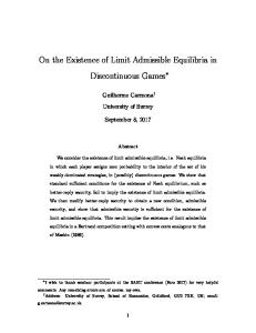
Consider the disturbed game Γ∗ (ϵ) obtained by attaching disturbances ϵr and ϵt to the payoffs associated to the pure strategies U and L respectively. The realization of the disturbances is private information. The domains Pr and Pt , in which the probability distributions of the ambiguous variables r and t lie, are common knowledge. Let their basic densities frb and ftb be the uniform densities on [−1, 1]: } { 1 − k 1 + kr  r ≤ f (x) ≤ for all x ∈ [−1, 1] , Pr := f ∈ F  2 2 } { 1 − k 1 + kt  t Pt := f ∈ F  ≤ f (x) ≤ for all x ∈ [−1, 1] . 2 2 We compute equilibrium strategies in the disturbed game, as a function of the ambiguity parameters kr and kt . As shown in Lemma 3, the strategy picked by player 2 will appear to player 1 as an Ellsberg strategy [qmin , qmax ]. By Lemma 4, her best reply to [qmin , qmax ] is a maxmin strategy characterized by two thresholds r1 and r2 . These two thresholds are illustrated in Figure 5. As shown in Lemma 9, for sufficiently small ϵ, a unique threshold value lies in the support of r. This threshold r∗ is the one associated with qmax , because q ∗ = 23 is the upper bound of the equilibrium Ellsberg strategy of player 2. The best reply to [qmin , qmax ] is a pure strategy whose threshold r∗ is obtained in equation (27). For player 2, the best reply to [pmin , pmax ] is a pure strategy whose threshold t∗ is obtained in equation (28). ϵr∗ = U1 (0, qmax ) − U1 (1, qmax ) = 3qmax − 2, ϵt∗ = U2 (0, pmax ) − U2 (1, pmax ) = 3pmax − 2.

(27) (28)

Thresholds r∗ and t∗ completely characterize the equilibrium strategies of the players for small disturbances. Our objective is therefore to compute their values as a function of the parameters of the game. 10

Our game Γ3 belongs to the set of games Riedel and Sass (2013) cover if one inverses the two columns. Therefore, Γ3 is such that p¯ ≤ p∗ and (1 − q)∗ ≤ (1 − q).

33

U1

U1 (p, qmin )

ϵr1 ϵr2 = ϵr∗

b

U1 (p, qmax ) b

b

p¯

0

p∗

b

p

1

Figure 5: Thresholds value r1 and r2 for a given Ellsberg strategy [qmin , qmax ].

By simplifying equation (14) in Lemma 5, we have:11 ∫

qmax

∫ 1 1 = max f (t)dt + 1f (t)dt f ∈Pt −1 3 t∗ ) ( 1 + kt ∗ 1 + kt 1 + (1 − t∗ ) 1 = 1 − (1 − t ) 2 3 2 ) 1( = 2 − t∗ (1 + kt ) + kt 3 t∗

Similarly, we obtain for pmax : ∫ r∗ ∫ 1 ) 1 1( pmax = max f (r)dr + 1f (r)dr = 2 − r∗ (1 + kr ) + kr f ∈Pr −1 3 3 r∗ Replacing in equations (27) and (28), the values of qmax and pmax found above, we obtain a system of two equations: { ∗ ϵr = kt − t∗ (1 + kt ), ϵt∗ = kr − r∗ (1 + kr ). Solving this system yields: {

r∗ = t∗ =

ϵkt −kr (1+kt ) , ϵ2 −(1+kr )(1+kt ) ϵkr −kt (1+kr ) . ϵ2 −(1+kt )(1+kr )

This last system of equations characterizes for small ϵ the equilibrium strategies in the disturbed game, as a function of the size of the disturbance ϵ and The second expression is valid when t∗ has a positive value, which is verified for small ϵ by equation (30). 11

34

the ambiguity parameters kr and kt . When the disturbance ϵ tends to 0, we have: kr , 1 + kr kt . lim t∗ = ϵ→0 1 + kt

lim r∗ = ϵ→0

4.2

(29) (30)

The sequence of equilibria

The equilibrium strategy of player 2, characterized by t∗ , is perceived by player 1 as an Ellsberg strategy [qmin , qmax ]. Alternatively, player 2 perceives the strategy of player 1 characterized by r∗ as an Ellsberg strategy [pmin , pmax ]. We computed above that: ) 1( 2 − t∗ (1 + kt ) + kt , 3 ) 1( = 2 − r∗ (1 + kr ) + kr . 3

qmax = pmax

(31) (32)

Similarly, we derive: ) 1( 2 − t∗ (1 − kt ) − kt , 3 ) 1( = 2 − r∗ (1 − kr ) − kr . 3

qmin = pmin

(33) (34)

Replacing in equations (31) to (34) variables t∗ and r∗ by their values allows to compute the sequence {e(ϵ)} of induced Ellsberg strategy profiles in the disturbed game Γ∗ (ϵ). Theorem 1 proved that for all proper equilibria e of Γ, we can find a pair (kr , kt ) ∈ [0, 1] × [0, 1] such that limϵ→0 {e(ϵ)} = e. Replacing r∗ and t∗ by their value in the limit, we obtain: ([ ] [ ]) ) ( 2 1 2 2 1 2 lim [pmin , pmax ], [qmin , qmax ] = , , , (35) ϵ→0 3 1 + kr 3 3 1 + kt 3 Remember that all) proper Ellsberg equilibrium of this game are of the form ( 2 e = [p1 , 3 ], [q1 , 23 ] with 31 ≤ p1 , q1 . For kr = 0, we have pmin = 32 and for kr = 1, we have pmin = 13 . Since function pmin is strictly monotone in kr between these two bounds, and since the same is true for function qmin and kt , any Ellsberg equilibrium in Γ3 can be disambiguated for a unique pair (kr , kt ).

35

5

Concluding Remarks

Riedel and Sass (2013) have introduced Ellsberg games and proposed a solution concept that they call Ellsberg equilibrium. It is a coarsening of Nash equilibrium. Any Nash equilibrium is an Ellsberg equilibrium but the converse does not hold: (quasi-) proper Ellsberg equilibria are not Nash equilibria. For the class of 2×2 normal form games that we consider, Harsanyi (1973) has shown that all Nash equilibria in mixed strategies can be purified. Our Disambiguation Theorem shows that all (quasi-) proper Ellsberg equilibria can be disambiguated. Moreover, for games of class I, all (quasi-) proper Ellsberg equilibria can be purified. In that sense, our result extends that of Harsanyi. Generalizing our theorem beyond 2×2 normal games can unfortunately not be done using the mathematical technique of Harsanyi. In effect, ambiguity averse players perform non-smooth evaluations of ambiguous outcomes. We can nevertheless see no fundamental reason why this generalization could not be performed, even though some challenging obstacles need to be overcome.

36

A

Appendix

A.1

Proof of Lemma 1

Proof. A proof of claim 1 can be found in Fudenberg and Tirole (1991). We prove claim 2: if player 1’s payoffs are not Column Dominant in game Γ then p¯ ∈ (0, 1) and U1 (¯ p, q) = U1 (¯ p, q ′ ) for all q, q ′ ∈ [0, 1]. Geometrically, given the strategy q chosen by player 2, the expected utility U1q (p) := U1 (p, q) defines a line in [0, 1] × R. If we allow the domain of q to be R, this line is defined in R2 . The family of such lines {U1q (p)}q∈[0,1] has the property of Unique Intersection. Property 1 (Unique Intersection). Let {U1q (p)}q∈[0,1] be a family of lines defined in R2 . The family has the property of unique intersection if there exists a point (˜ p, u1 ) ∈ R2 at which all members of the family intersect. This unique intersection (˜ p, u1 ) is hence such that for all q ∈ [0, 1], the q point (˜ p, u1 ) ∈ U1 (p). We show now that family {U1q (p)}q∈[0,1] has a unique intersection (˜ p, u1 ). Player 1’s expected utility can be rewritten: ( ) U1 (p, q) = π14 + q (π13 − π14 ) + p(π11 − π12 − π13 + π14 ) + p(π12 − π14 ). The value p˜ at which an intersection takes place is therefore the solution of the following equation: (π13 − π14 ) + p˜(π11 − π12 − π13 + π14 ) = 0. As there are no weakly dominant strategies in Γ, player 1’s payoff are not Row Dominant and hence two cases can arise. • Case A: π11 > π13 and π12 < π14 . The solution p˜ of last equation belongs to (0, 1) if either π11 > π12 and π13 < π14 or π11 < π12 and π13 > π14 . This means p˜ ∈ (0, 1) if player 1’s payoff are not Column Dominant. Therefore the factor π11 −π12 −π13 +π14 is different from zero. As a result the solution p˜ is unique. • Case B: π11 < π13 and π12 > π14 A parallel argument can be made to show p˜ ∈ (0, 1) and is unique. We now prove for games with p˜ ∈ (0, 1) that this intersection is the maxmin strategy, that is p˜ = p¯. By definition of indifference strategy q ∗ , we ∗ have for all p ∈ [0, 1] that U1 (p, q ∗ ) = U1 (˜ p, q ∗ ) = u1 and hence U1q (p) is flat: 37

U1 (0, q ∗ ) − U1 (1, q ∗ ) = 0. As player 1 has no weakly dominant strategy, the difference U1 (0, q) − U1 (1, q) is strictly monotone in q. This implies q ∗ is the only value for which U1q (p) is flat. We showed that q ∗ ∈ (0, 1), implying there exist hence q ′ and q ′′ in [0, 1] such that q ′ < q ∗ < q ′′ . By strict monotonicity of ′ the difference U1 (0, q)−U1 (1, q), we have that among the two lines U1q (p) and ′′ U1q (p), one is strictly increasing and the other strictly decreasing. Therefore, as p˜ ∈ (0, 1), for any p ∈ [0, 1] with p ̸= p˜ there exists q ∈ [0, 1] with q ̸= q ∗ such that U1q (p) < U1q (˜ p). The maxmin strategy p¯ is hence at the intersection p˜. This completes the proof as we showed that utility in p˜ is independent of q. The proof of claim 3 is done using the same argument. ■

A.2

Proof of Lemma 2

Proof. We assume without loss of generality that p1 < p2 . First, we show q ∗ ∈ {q1 , q2 }. As shown in Lemma 1, for all Γ ∈ Γ, we have that q ∗ ∈ (0, 1) and is unique. The Ellsberg strategy [p1 , p2 ] is a best reply to [q1 , q2 ], if and if we have(for all p )∈ [p1 , p2 ] there exists no p′ ∈ [0, 1] such that ( only ) U1 p′ , [q1 , q2 ] > U1 p, [q1 , q2 ] . Being ambiguity averse, player 1 must be indifferent between all mixed strategies inside the Ellsberg strategy [p1 , p2 ] she plays. Formally, for all p, p′ ∈ [p1 , p2 ] we have ( ) ( ) U1 p′ , [q1 , q2 ] = U1 p, [q1 , q2 ] . ( ) ( ) As U1 p, [q1 , q2 ] = min U1 (p, q1 ), U1 (p, q2 ) (equation (1)), we must have either • U1 (p, q1 ) is constant (implying q1 = q ∗ ) and U1 (p, q1 ) ≤ U1 (p, q2 ) for all p ∈ [p1 , p2 ], or • U1 (p, q2 ) is constant (implying q2 = q ∗ ) and U1 (p, q2 ) ≤ U1 (p, q1 ) for all p ∈ [p1 , p2 ]. Therefore we have q ∗ ∈ {q1 , q2 }. Second, we show p∗ ∈ {p1 , p2 }. If [q1 , q2 ] is a proper Ellsberg strategy, then the reasoning above proves it. We show it holds as well if the equilibrium is quasi-proper, that is q1 = q2 . From the previous reasoning, this implies q1 = q2 = q ∗ . The Ellsberg strategy q ∗( is a best reply to( [p1 , p2 ], if)and only if there ) ′ ′ ∗ exists no( q ∈ [0, 1]) such that ( U2 q , [p1 , p2 ] >) U2 q , [p1 , p2 ] . Remember we have U2 q, [p1 , p2 ] = min U2 (q, p1 ), U2 (q, p2 ) . Function U2 (q, p) is linear in q. We show that if p∗ ∈ / {p1 , p2 }, we have a contradiction.

38

• If U2 (q, [p1 , p2 ]) is strictly increasing in q on [0, 1], then best reply is q1 = q2 = 1, and since q ∗ ̸= 1 for all Γ ∈ Γ, we have a contradiction. • If U2 (q, [p1 , p2 ]) is strictly decreasing in q on [0, 1], then best reply is q1 = q2 = 0, and since q ∗ ̸= 0, we have another contradiction. • If U2 (q, [p1 , p2 ]) is strictly increasing in q on one portion of [0, 1] and stricly decreasing on the other, then the best reply is q¯. In effect, by the property of Unique Intersection, U2 (q, p1 ) and U2 (q, p2 ) must then intersect in (¯ q , u2 ) and U2 (q, [p1 , p2 ]) has maximal value for q = q¯. As for all Γ ∈ Γ, q ∗ ̸= q¯, we have yet another contradiction. The only possibility for q ∗ to belong to best replies is that either U2 (q, p1 ) or U2 (q, p2 ) is constant in q, which implies p∗ ∈ {p1 , p2 }. ■

A.3

Proof of Lemma 3

Proof. We show that for all p ∈ [pmin , pmax ], there exists a density f ∈ Pr such that ∫ 1 p= pb (r)f (r)dr. −1

The domain Pr is convex. This means that for all f1 , f2 ∈ Pr , distribution f∫3 defined as f3 (r) := λf1 (r) + (1 − λ)f2 (r) belongs to Pr . The mapping 1 pb (r)f (r)dr is linear in f . As the image of a convex set through a linear −1 mapping is a convex set, the image of Pr through this mapping is convex. In the [real line, a] convex set is an interval. As Pr is closed, so must be its image pmin , pmax . ■

A.4

Best replies in disturbed game

For all Γ ∈ Γ such that player 1’s payoffs are Column Dominant, the following lemma provides conditions under which a pure strategy of player 1 is a best reply to a strategy of player 2 inducing [qmin , qmax ].12 Lemma 13 (Best-Reply in pure strategy). For all ϵ > 0 and all Γ ∈ Γ such that player 1’s payoffs are Column Dominant, the strategy pb is a best reply to any [qmin , qmax ] ⊆ [0, 1] if it is a pure In Lemma 13, the conditions under which the expression max(r′ , r′′ ) is used for r∗ are such that the solution p of the implicit equation U1 (p, 0) = U1 (p, 1) is non-positive. The conditions under which the expression min(r′ , r′′ ) is used for r∗ are such that the solution p of the implicit equation U1 (p, 0) = U1 (p, 1) is equal or larger than 1. 12

39

1 strategy pb = r∗ ∈ Spu defined by:

ϵr′ = U1 (0, qmin ) − U1 (1, qmin ), ϵr′′ = U1 (0, qmax ) − U1 (1, qmax ), { max(r′ , r′′ ) if |π13 − π14 | ≤ |π11 − π12 |, ∗ r = ′ ′′ min(r , r ) otherwise. Proof. The proof is only provided for the conditions on player 1’s payoffs leading to r∗ = max(r′ , r′′ ). Those conditions ensure that the solution to equation (π13 − π14 ) + p(π11 − π12 − π13 + π14 ) = 0, which yields the unique intersection p˜, is non-positive. Therefore the relevant threshold among r′ and r′′ is the largest one.13 Take any ϵ > 0, any [qmin , qmax ] ⊆ [0, 1] and any Γ ∈ Γ such that • player 1’s payoffs are Column Dominant, and • the solution to equation (π13 − π14 ) + p(π11 − π12 − π13 + π14 ) = 0 is nonpositive. Given equations (1) and (2), we have ( ) ( ) U1 p, [qmin , qmax ], ϵr = min U1 (p, qmin , ϵr), U1 (p, qmax , ϵr) ( ) = min U1 (p, qmin ) + pϵr, U1 (p, qmax ) + pϵr where U1 (p, q, ϵr) is linear in p since U1 (p, q) is linear in p. For the considered Γ, p¯ is not a proper mixed strategy and the unique intersection of U1 (p, q1 ) and U1 (p, q2 ) is in (˜ p, u1 ) with p˜ ≤ 0. Therefore, if qmin ̸= qmax , we have two possible cases: • Case A: U1 (p, qmin ) > U1 (p, qmax ) for all p ∈ (0, 1), • Case B: U1 (p, qmin ) < U1 (p, qmax ) for all p ∈ (0, 1). Let qˆ := qmax if we are in case A and qˆ := qmin if we are in case B. The mixed strategy qˆ ∈ {qmin , qmax } is the one associated with the minimal utility for player 1, the one she takes into account in front of ambiguity. We have hence ( ) U1 p, [qmin , qmax ], ϵr = U1 (p, qˆ) + pϵr. If qmin = qmax then r∗ = r′ = r′′ . But if qmin < qmax , two cases can arise: either U1 (p, qmin ) < U1 (p, qmax ) for all p ∈ (0, 1] or U1 (p, qmin ) > U1 (p, qmax ) for all p ∈ (0, 1]. Assume that the game Γ is such that the first of these two cases arises. The relevant threshold r∗ is therefore r′ associated to qmin . Under the payoff conditions leading to r∗ = max(r′ , r′′ ), U1 (p, qmin ) and U1 (p, qmax ) are two straight lines which cross at p˜ ≤ 0. As a result, we have U1 (0, qmin ) − U1 (1, qmin ) > U1 (0, qmax ) − U1 (1, qmax ). The other case leads to the same conclusion. 13

40

From the definition of qˆ and the definition of r∗ in the statement of the lemma, we have ϵr∗ = U1 (0, qˆ) − U1 (1, qˆ), which can be rewritten U1 (0, qˆ) + 0ϵr∗ = U1 (1, qˆ) + 1ϵr∗ implying that: 1. U1 (0, qˆ) + 0ϵr > U1 (1, qˆ) + 1ϵr for all r < r∗ , 2. U1 (0, qˆ) + 0ϵr < U1 (1, qˆ) + 1ϵr for all r > r∗ . As U1 (p, qˆ) + pϵr is a linear function of p, the best reply to all r < r∗ is p = 0 and the best reply to all r > r∗ is p = 1. If r = r∗ then U1 (p, qˆ) + pϵr is a constant and any p ∈ [0, 1] is a best reply, and in particular p = 0. ■ For all Γ ∈ Γ such that player 2’s payoffs are Row Dominant, there exists similar conditions under which a pure strategy of player 2 is a best reply to a strategy of player 1 inducing [pmin , pmax ].14 For for all Γ ∈ Γ such that player 2’s payoffs are Row Dominant, those conditions are obtained for pure strategies of player 2 by replacing π11 by π21 , π14 by π24 , π12 by π23 and π13 by π22 . 14

41

References Camerer, C. and Weber, M. (1992). Recent developments in modeling preferences: Uncertainty and ambiguity. Journal of Risk and Uncertainty, 5(4):325–370. Eichberger, J. and Kelsey, D. (2000). Non-Additive Beliefs and Strategic Equilibria. Games and Economic Behavior, 30(2):183–215. Fudenberg, D. and Tirole, J. (1991). Game Theory. MIT Press. Gajdos, T., Hayashi, T., Tallon, J.-M., and Vergnaud, J.-C. (2008). Attitude toward imprecise information. Journal of Economic Theory, 140(1):27–65. Gilboa, I. and Schmeidler, D. (1989). Maximin Expected Utility with nonUnique Priors. Journal of Mathematical Economics, 18(2):141 – 153. Greenberg, J. (2000). The right to remain silent. Theory and Decision, 48(2):193–204. Harsanyi, J. C. (1973). Games with randomly disturbed payoffs: A new rationale for mixed-strategy equilibrium points. International Journal of Game Theory, 2(1):1–23. Huber, P., J. (1981). Robust Statistics. John Wiley, New-York. Lo, K. C. (1996). Equilibrium in Beliefs under Uncertainty. Journal of Economic Theory, 71(2):443–484. Maccheroni, F., Marinacci, M., and Rustichini, A. (2006). Ambiguity aversion, robustness, and the variational representation of preferences. Econometrica, 74(6):1447–1498. Marinacci, M. (2000). Ambiguous Games. Games and Economic Behavior, 31(2):191–219. Neumann, J. V. (1928). Zur Theorie der Gesellschaftsspiele. Mathematische Annalen, 100(1):295–320. Riedel, F. and Sass, L. (2013). 76(4):469–509.

Ellsberg games.

Theory and Decision,

Schelling, T. C. (1980). The strategy of conflict. Harvard university press.

42