Disambiguating Toponyms in News Eric Garbin
Inderjeet Mani
Department of Linguistics Georgetown University Washington, DC 20057, USA
[email protected]
Department of Linguistics Georgetown University Washington, DC 20057, USA
[email protected]
Abstract This research is aimed at the problem of disambiguating toponyms (place names) in terms of a classification derived by merging information from two publicly available gazetteers. To establish the difficulty of the problem, we measured the degree of ambiguity, with respect to a gazetteer, for toponyms in news. We found that 67.82% of the toponyms found in a corpus that were ambiguous in a gazetteer lacked a local discriminator in the text. Given the scarcity of humanannotated data, our method used unsupervised machine learning to develop disambiguation rules. Toponyms were automatically tagged with information about them found in a gazetteer. A toponym that was ambiguous in the gazetteer was automatically disambiguated based on preference heuristics. This automatically tagged data was used to train a machine learner, which disambiguated toponyms in a human-annotated news corpus at 78.5% accuracy.
1 Introduction Place names, or toponyms, are ubiquitous in natural language texts. In many applications, including Geographic Information Systems (GIS), it is necessary to interpret a given toponym mention as a particular entity in a geographical database or gazetteer. Thus the mention “Washington” in “He visited Washington last year” will need to be interpreted as a reference to either the city Washington, DC or the U.S. state of Washington, and “Berlin” in “Berlin is cold in the winter” could
mean Berlin, New Hampshire or Berlin, Germany, among other possibilities. While there has been a considerable body of work distinguishing between a toponym and other kinds of names (e.g., person names), there has been relatively little work on resolving which place and what kind of place given a classification of kinds of places in a gazetteer. Disambiguated toponyms can be used in a GIS to highlight a position on a map corresponding to the coordinates of the place, or to draw a polygon representing the boundary. In this paper, we describe a corpus-based method for disambiguating toponyms. To establish the difficulty of the problem, we began by quantifying the degree of ambiguity of toponyms in a corpus with respect to a U.S. gazetteer. We then carried out a corpus-based investigation of features that could help disambiguate toponyms. Given the scarcity of human-annotated data, our method used unsupervised machine learning to develop disambiguation rules. Toponyms were automatically tagged with information about them found in a gazetteer. A toponym that was ambiguous in the gazetteer was automatically disambiguated based on preference heuristics. This automatically tagged data was used to train the machine learner. We compared this method with a supervised machine learning approach trained on a corpus annotated and disambiguated by hand. Our investigation targeted toponyms that name cities, towns, counties, states, countries or national capitals. We sought to classify each toponym as a national capital, a civil political/administrative region, or a populated place (administration unspecified). In the vector model of GIS, the type of place crucially determines the geometry chosen to represent it (e.g., point, line or polygon) as well as any reasoning about geographical inclusion. The class of the toponym can be useful in “grounding” the toponym to latitude and longitude coordinates,
Entry Number
Topony m
U.S. County
U.S. State
110
Acton
Middlesex
Massachusetts Montana
112
but it can also go beyond grounding to support spatial reasoning. For example, if the province is merely grounded as a point in the data model (e.g., if the gazetteer states that the centroid of a province is located at a particular latitude-longitude) then without the class information, the inclusion of a city within a province can’t be established. Also, resolving multiple cities or a unique capital to a political region mentioned in the text can be a useful adjunct to a map that lacks political boundaries or whose boundaries are dated. It is worth noting that our classification is more fine-grained than efforts like the EDT task in Automatic Content Extraction1 program (Mitchell and Strassel 2002), which distinguishes between toponyms that are a Facility “Alfredo Kraus Auditorium”, a Location “the Hudson River”, and GeoPolitical Entities that include territories “U.S. heartland”, and metonymic or other derivative place references “Russians”, “China (offered)”, “the U.S. company”, etc. Our classification, being gazetteer based, is more suited to GIS-based applications.
2 Quantifying Toponym Ambiguity Data
We used a month’s worth of articles from the New York Times (September 2001), part of the English Gigaword (LDC 2003). This corpus consisted of 7,739 documents and, after SGML stripping, 6.51 million word tokens with a total size of 36.4MB). We tagged the corpus using a list of place names from the USGS Concise Gazetteer (GNIS). The resulting corpus is called MAC1, for “Machine Annotated Corpus 1”. GNIS covers cities, states, 1
Elevation (ft. Class above sea level) 260 Ppl (populated place) 3816 Ppl
422906N0712600W Acton Yellow455550Nstone 1084048W Acton Los Ange- California 342812N2720 les 1181145W Table 1. Example GNIS entries for an ambiguous toponym
111
2.1
Lat-Long (dddmmss)
www.ldc.upenn.edu/Projects/ACE/
Ppl
and counties in the U.S., which are classified as “civil” and “populated place” geographical entities. A geographical entity is an entity on the Earth’s surface that can be represented by some geometric specification in a GIS; for example, as a point, line or polygon. GNIS also covers 53 other types of geo-entities, e.g., “valley,” “summit”, “water” and “park.” GNIS has 37,479 entries, with 27,649 distinct toponyms, of which 13,860 toponyms had multiple entries in the GNIS (i.e., were ambiguous according to GNIS). Table 1 shows the entries in GNIS for an ambiguous toponym. 2.2
Analysis
Let E be a set of elements, and let F be a set of features. We define a feature g in F to be a disambiguator for E iff for all pairs
in E X E, g(ex) ≠ g(ey) and neither g(ex) nor g(ey) are nullvalued. As an example, consider the GNIS gazetteer in Table 1, let F = {U.S. County, U.S. State, Lat-Long, and Elevation}. We can see that each feature in F is a disambiguator for the set of entries E = {110, 111, 112}. Let us now characterize the mapping between texts and gazetteers. A string s1 in a text is said to be a discriminator within a window w for another string s2 no more than w words away if s1 matches a disambiguator d for s2 in a gazetteer. For example, “MT” is a discriminator within a window 5 for the toponym “Acton” in “Acton, MT,” since “MT” occurs within a ±5-word window of “Acton” and matches, via an abbreviation, “Montana”, the value of a GNIS disambiguator U.S. State (here the tokenized words are “Acton”, “,”, and “MT”). A trie-based lexical lookup tool (called LexScan) was used to match each toponym in GNIS against the corpus MAC1. Of the 27,649 distinct toponyms
in GNIS, only 4553 were found in the corpus (note that GNIS has only U.S. toponyms). Of the 4553 toponyms, 2911 (63.94%) were “bare” toponyms, lacking a local discriminator within a ±5-word window that could resolve the name. Of the 13,860 toponyms that were ambiguous according to GNIS, 1827 of them were found in MAC1, of which only 588 had discriminators within a ±5-word window (i.e., discriminators which matched gazetteer features that disambiguated the toponym). Thus, 67.82% of the 1827 toponyms found in MAC1 that were ambiguous in GNIS lacked a discriminator. This 67.82% proportion is only an estimate of true toponym ambiguity, even for the sample MAC1. There are several sources of error in this estimate: (i) World cities, capitals and countries were not yet considered, since GNIS only covered U.S. toponyms. (ii) In general, a single feature (e.g., County, or State) may not be sufficient to disambiguate a set of entries. It is of course possible for two different places named by a common toponym to be located in the same county in the same state. However, there were no toponyms with this property in GNIS. (iii) A string in MAC1 tagged by GNIS lexical lookup as a toponym may not have been a place name at all (e.g., “Lord Acton lived …”). Of the toponyms that were spurious, most were judged by us to be common words and person names. This should not be surprising, as 5341 toponyms in GNIS are also person names according to the U.S. Census Bureau2 (iv) LexScan wasn’t perfect, for the following reasons. First, it sought only exact matches. Second, the matching relied on expansion of standard abbreviations. Due to non-standard abbreviations, the number of true U.S. toponyms in the corpus likely exceeded 4553. Third, the matches were all case-sensitive: while case-insensitivity caused numerous spurious matches, case-sensitivity missed a more predictable set, i.e. all-caps dateline toponyms or lowercase toponyms in Internet addresses. Note that the 67.82% proportion is just an estimate of local ambiguity. Of course, there are often non-local discriminators (outside the ±5-word windows); for example, an initial place name reference could have a local discriminator, with sub2
www.census.gov/genealogy/www/freqnames.html
sequent references in the article lacking local discriminators while being coreferential with the initial reference. To estimate this, we selected cases where a toponym was discriminated on its first mention. In those cases, we counted the number of times the toponym was repeated in the same document without the discriminator. We found that 73% of the repetitions lacked a local discriminator, suggesting an important role for coreference (see Sections 4 and 5).
3 Knowledge Sources for Automatic Disambiguation To prepare a toponym disambiguator, we required a gazetteer as well as corpora for training and testing it. 3.1
Gazetteer
To obtain a gazetteer that covered worldwide information, we harvested countries, country capitals, and populous world cities from two websites ATLAS3 and GAZ4, to form a consolidated gazetteer (WAG) with four features G1,..,G4 based on geographical inclusion, and three classes, as shown in Table 2. As an example, an entry for Aberdeen could be the following feature vector: G1=United States, G2=Maryland, G3=Harford County, G4=Aberdeen, CLASS=ppl. We now briefly discuss the merging of ATLAS and GAZ to produce WAG. ATLAS provided a simple list of countries and their capitals. GAZ recorded the country as well as the population of 700 cities of at least 500,000 people. If a city was in both sources, we allowed two entries but ordered them in WAG to make the more specific type (e.g. “capital”) the default sense, the one that LexScan would use. Accents and diacritics were stripped from WAG toponyms by hand, and aliases were associated with standard forms. Finally, we merged GNIS state names with these, as well as abbreviations discovered by our abbreviation expander. 3.2
Corpora
We selected a corpus consisting of 15,587 articles from the complete Gigaword Agence France 3 4
. www.worldatlas.com www.worldgazetteer.com
Presse, May 2002. LexScan was used to tag, insensitive to case, all WAG toponyms found in this corpus, with the attributes in Table 2. If there were
multiple entries in WAG for a toponym, LexScan only tagged the preferred sense, discussed below. The resulting tagged corpus, called MAC-DEV,
Tag At- Description tribute CLASS Civil (Political Region or Administrative Area, e.g. Country, Province, County), Ppl (Populated Place, e.g. City, Town), Cap (Country Capital, Provincial Capital, or County Seat) G1 Country G2 Province (State) or Country-Capital G3 County or Independent City G4 City, Town (Within County) Table 2: WAG Gazetteer Attributes Corpus MAC1 MACDEV MACML HAC
Size 6.51 million words with 61,720 place names (4553 distinct) from GNIS 5.47 million words with 124,175 place names (1229 distinct) from WAG 6.21 million words with 181,866 place names (1322 distinct) from WAG 83,872 words with 1275 place names (435 distinct) from WAG.
Use Ambiguity Study (Gigaword NYT Sept. 2001) (Section 2) Development Corpus (Gigaword AFP May 2002) (Section 4) Machine Learning Corpus (Gigaword AP Worldwide January 2002) (Section 5) Human Annotated Corpus (from TimeBank 1.2, and Gigaword NYT Sept. 2001 and June 2002) (Section 5)
How Annotated LexScan of all senses, no attributes marked LexScan using attributes from WAG, with heuristic preference LexScan using attributes from WAG, with heuristic preference LexScan using WAG, with attributes and sense being manually corrected
Table 3. Summary of Corpora Term found T-test with Cap Civil ‘stock’ ‘exchange’ ‘embassy’ ‘capital’ ‘airport’ ‘summit’ ‘lower’ ‘visit’ ‘conference’ ‘agreement’
4 4.24 3.61 1.4 3.32 4 3.16 4.61 4.24 3.16
TTerm found T-test T-test Term found test with Ppl Civil Cap with Civil Ppl 4 ‘winter’ 3.61 3.61 ‘air’ 4.24 ‘telephone’ 3.16 3.16 ‘base’ 3.61 ‘port’ 3.46 3.46 ‘accuses’ ‘midfielder’ 3.46 3.46 ‘northern’ 2.2 3.32 ‘city’ 1.19 1.19 ‘airlines’ 4 ‘invaded’ ‘near’ 2.77 3.83 3.16 ‘times’ 3.16 3.16 ‘southern’ ‘southern’ 3.87 3.87 ‘friendly’ 4.69 4.24 ‘state-run’ ‘yen’ 4 0.56 3.16 ‘border’ ‘attack’ 0.18 3.87 Table 4. Top 10 terms disambiguating toponym classes
was used as a development corpus for feature exploration. To disambiguate the sense for a
Ttest Ppl 3.16 3.16 3.61 5.57 4.8 3.32 3.87 4 3.32 7.48
T-test Cap 3.16 3.16 3.61 5.57 4.8 3.32 6.71 4 3.32 7.48
toponym that was ambiguous in WAG, we used two preference heuristics. First, we searched
MAC1 for two dozen highly frequent ambiguous toponym strings (e.g., “Washington”, etc.), and observed by inspection which sense predominated in MAC1, preferring the predominant sense for each of these frequently mentioned toponyms. For example, in MAC1, “Washington” was predominantly a Capital. Second, for toponyms outside this most frequent set, we used the following specificity-based preference: Cap. > Ppl > Civil. In other words, we prefer the more specific sense; since there are a smaller number of Capitals than Populated places, we prefer Capitals to Populated Places. For machine learning, we used the Gigaword Associated Press Worldwide January 2002 (15,999 articles), tagged in the same way by LexScan as MAC-DEV was. This set was called MAC-ML. Thus, MAC1, MAC-DEV, and MAC-ML were all generated automatically, without human supervision. For a blind test corpus with human annotation, we opportunistically sampled three corpora: MAC1, TimeBank 1.25 and the June 2002 New York Times from the English Gigaword, with the first author tagging a random 28, 88, and 49 documents respectively from each. Each tag in the resulting human annotated corpus (HAC) had the WAG attributes from Table 2 with manual correction of all the WAG attributes. A summary of the corpora, their source, and annotation status is shown in Table 3.
4 Feature Exploration We used the tagged toponyms in MAC-DEV to explore useful features for disambiguating the classes of toponyms. We identified single-word terms that co-occurred significantly with classes within a k-word window (we tried k= ±3, and k=±20). These terms were scored for pointwise mutual information (MI) with the classes. Terms with average tf.idf of less than 4 in the collection were filtered out as these tended to be personal pronouns, articles and prepositions. To identify which terms helped select for particular classes of toponyms, the set of 48 terms whose MI scores were above a threshold (-11, chosen by inspection) were filtered using the student’s t-statistic, based on an idea in (Church 5
www.timeml.org
and Hanks 1991). The t-statistic was used to compare the distribution of the term with one class of toponym to its distribution with other classes to assess whether the underlying distributions were significantly different with at least 95% confidence. The results are shown in Table 4, where scores for a term that occurred jointly in a window with at least one other class label are shown in bold. A t-score > 1.645 is a significant difference with 95% confidence. However, because joint evidence was scarce, we eventually chose not to eliminate Table 4 terms such as ‘city’ (t =1.19) as features for machine learning. Some of the terms were significant disambiguators between only one pair of classes, e.g. ‘yen,’ ‘attack,’ and ‘capital,’ but we kept them on that basis. Feature Name Abbrev
Description
Value is true iff the toponym is abbreviated. Value is true iff the AllCaps toponym is all capital letters. Values are the ordered Left/Right tokens up to k positions to Pos{1,.., k} the left/right Value is the set of MI WkContext collocated terms found in windows of ± k tokens (to the left and right) Value is the set of TagDisCLASS values represented course by all toponyms from the document: e.g., the set {civil, capital, ppl} Value is the CLASS if CorefClass any for a prior mention of a toponym in the document, or none Table 5. Features for Machine Learning Based on the discovered terms in experiments with different window sizes, and an examination of MAC1 and MAC-DEV, we identified a final set of features that, it seemed, might be useful for machine learning experiments. These are shown in Table 5. The features Abbrev and Allcaps describe evidence internal to the toponym:
an abbreviation may indicate a state (Mass.), territory (N.S.W.), country (U.K.), or some other civil place; an all-caps toponym might be a capital or ppl in a dateline. The feature sets LeftPos and RightPos target the ±k positions in each window as ordered tokens, but note that only windows with a MI term are considered. The domain of WkContext is the window of ±k tokens around a toponym that contains a MI collocated term. We now turn to the global discourse-level features. The domain for TagDiscourse is the whole document, which is evaluated for the set of toponym classes present: this information may reflect the discourse topic, e.g. a discussion of U.S. sports teams will favor mentions of cities over states or capitals. The feature CorefClass
implements a one sense per discourse strategy, motivated by our earlier observation (from Section 2) that 73% of subsequent mentions of a toponym that was discriminated on first mention were expressed without a local discriminator.
5 Machine Learning The features in Table 5 were used to code feature vectors for a statistical classifier. The results are shown in Table 6. As an example, when the Ripper classifier (Cohen 1996) was trained on MAC-ML with a window of k= ±3 word tokens, the predictive accuracy when tested using crossvalidation MAC-ML was 88.39% ±0.24 (where 0.24 is the standard deviation across 10 folds).
Accuracy on Test Set Window = ±3 Training
Test Set
Set MAC-ML
MAC-DEV
MAC-DEV
HAC
MACDEV+MACML MACDEV+MACML
Window = ±20
Predictive
Recall, Preci-
Predictive Recall, Precision,
Accuracy
sion, F-measure
Accuracy
F-measure
80.97 ± Cap r61 p77 f68 0.33 (Civ. Civ. r83 p86 f84 Ppl r81 p72 f76 57.1) Avg. r75 p78 f76 MAC-DEV 81.36 ± Cap r49 p78 f60 (cross0.59 (Civ. Civ. r92 p81 f86 Ppl r56 p70 f59 validation) 59.3) Avg. r66 p77 f68 65.33 Cap r100 p100 HAC (Civ. 50.7) f100 Civ. r84 p62 f71 Ppl r43 p71 f54 Avg. r76 p78 f75 HAC 77.5 ± 2.94 Cap r70 p97 f68 73.12 ± Cap r17 p90 f20 Civ. r34 p94 f49 (Ppl 72.9) (cross3.09 (Ppl Civ. r63 p76 f68 Ppl r84 p73 f77 Ppl r98 p64 f77 validation) 51.3) Avg. r54 p79 f55 Avg. r67 p85 f65 Cap r56 p73 f63 Cap r70 p89 f78 MAC79.70 ± 86.76 ± DEV+MAC0.30 (Civ. Civ. r83 p86 f84 0.18 (Civ. Civ. r94 r88 f91 Ppl r80 p68 f73 Ppl r81 p80 f80 ML (cross- 60.7) 59.7) Avg. r73 p76 f73 Avg. r82 p86 f83 validation) Cap r100 p63 f77 HAC 73.07 (Civ. Cap r71 p83 f77 78.30 (Civ. 50) Civ. r91 p75 f82 Civ. r91 p69 f79 51.7) Ppl r63 p88 f73 Ppl r45 f81 f58 Avg. r85 p75 f77 Avg. r69 p78 f71 Table 6. Machine Learning Accuracy MAC-ML (crossvalidation)
88.39 ± Cap r70 p88 f78 0.24 (Civ. Civ. r94 p90 f92 65.0) Ppl r87 p82 f84 Avg. r84 p87 f85 87.08 ± Cap r74 p87 f80 0.28 (Civ. Civ. r93 p88 f91 57.8) Ppl r82 p80 f81 Avg. r83 p85 f84 68.66 (Civ. Cap r50 p71 f59 59.7) Civ. r93 p70 f80 Ppl r24 p57 f33 Avg. r56 p66 f57
The majority class (Civil) had the predictive accuracy shown in parentheses. (When tested on a different set from the training set, cross-validation wasn’t used). Ripper reports a confusion matrix for each class; Recall, Precision, and F-measure for these classes are shown, along with their average across classes. In all cases, Ripper is significantly better in predictive accuracy than the majority class. When testing using cross-validation on the same machine-annotated corpus as the classifier was trained on, performance is comparable across corpora, and is in the high 80%, e.g., 88.39 on MAC-ML (k=±3). Performance drops substantially when we train on machine-annotated corpora but test on the human-annotated corpus (HAC) (the unsupervised approach), or when we both train and test on HAC (the supervised approach). The noise in the autogenerated classes in the machine-annotated corpus is a likely cause for the lower accuracy of the unsupervised approach. The poor performance of the supervised approach can be attributed to the lack of human-annotated training data: HAC is a small, 83,872-word corpus. Rule Description (Window = ±3)
Coverage of Examples in Testing (Accuracy) 5/67 (100%)
If not AllCaps(P) and RightPos1(P,‘SINGLE_QUOTE’) and Civil ∈ TagDiscourse Then Civil(P). If not AllCaps(P) and Left13/67 (100%) Pos1(P, southern) and Civil ∈ TagDiscourse Then Civil(P). Table 7. Sample Rules Learnt by Ripper
TagDiscourse was a critical feature; ignoring it during learning dropped the accuracy nearly 9 percentage points. This indicates that prior mention of a class increases the likelihood of that class. (Note that when inducing a rule involving a set-valued feature, Ripper tests whether an element is a member of that set-valued feature, selecting the test that maximizes information gain for a set of examples.) Increasing the window size only lowered accuracy when tested on the same corpus (using crossvalidation); for example, an increase from ±3 words to ±20 words (intervening sizes are not shown for reasons of space) lowered the PA by 5.7
percentage points on MAC-DEV. However, increasing the training set size was effective, and this increase was more substantial for larger window sizes: combining MAC-ML with MAC-DEV improved accuracy on HAC by about 4.5% for k= ±3, but an increase of 13% was seen for k =±20. In addition, F-measure for the classes was steady or increased. As Table 6 shows, this was largely due to the increase in recall on the non-majority classes. The best performance when training Ripper on the machine-annotated MAC-DEV+MACML and testing on the human-annotated corpus HAC was 78.30. Another learner we tried, the SMO supportvector machine from WEKA (Witten and Frank 2005), was marginally better, showing 81.0 predictive accuracy training and testing on MACDEV+MAC-ML (ten-fold cross-validation, k=±20) and 78.5 predictive accuracy training on MACDEV+MAC-ML and testing on HAC (k=±20). Ripper rules are of course more transparent: example rules learned from MAC-DEV are shown in Table 7, along with their coverage of feature vectors and accuracy on the test set HAC.
6 Related Work Work related to toponym tagging has included harvesting of gazetteers from the Web (Uryupina 2003), hand-coded rules to place name disambiguation, e.g., (Li et al. 2003) (Zong et al. 2005), and machine learning approaches to the problem, e.g., (Smith and Mann 2003). There has of course been a large amount of work on the more general problem of word-sense disambiguation, e.g., (Yarowsky 1995) (Kilgarriff and Edmonds 2002). We discuss the most relevant work here. While (Uryupina 2003) uses machine learning to induce gazetteers from the Internet, we merely download and merge information from two popular Web gazetteers. (Li et al. 2003) use a statistical approach to tag place names as a LOCation class. They then use a heuristic approach to location normalization, based on a combination of handcoded pattern-matching rules as well as discourse features based on co-occurring toponyms (e.g., a document with “Buffalo”, “Albany” and “Rochester” will likely have those toponyms disambiguated to New York state). Our TagDiscourse feature is more coarse-grained. Finally, they assume one sense per discourse in their rules, whereas we use it
as a feature CorefClass for use in learning. Overall, our approach is based on unsupervised machine learning, rather than hand-coded rules for location normalization. (Smith and Mann 2003) use a “minimally supervised” method that exploits as training data toponyms that are found locally disambiguated, e.g., “Nashville, Tenn.”; their disambiguation task is to identify the state or country associated with the toponym in test data that has those disambiguators stripped off. Although they report 87.38% accuracy on news, they address an easier problem than ours, since: (i) our earlier local ambiguity estimate suggests that as many as two-thirds of the gazetteer-ambiguous toponyms may be excluded from their test on news, as they would lack local discriminators (ii) the classes our tagger uses (Table 3) are more fine-grained. Finally, they use one sense per discourse as a bootstrapping strategy to expand the machine-annotated data, whereas in our case CorefClass is used as a feature. Our approach is distinct from other work in that it firstly, attempts to quantify toponym ambiguity, and secondly, it uses an unsupervised approach based on learning from noisy machine-annotated corpora using publicly available gazetteers.
7 Conclusion This research provides a measure of the degree of of ambiguity with respect to a gazetteer for toponyms in news. It has developed a toponym disambiguator that, when trained on entirely machine annotated corpora that avail of easily available Internet gazetteers, disambiguates toponyms in a human-annotated corpus at 78.5% accuracy. Our current project includes integrating our disambiguator with other gazetteers and with a geovisualization system. We will also study the effect of other window sizes and the combination of this unsupervised approach with minimally-supervised approaches such as (Brill 1995) (Smith and Mann 2003). To help mitigate against data sparseness, we will cluster terms based on stemming and semantic similarity. The resources and tools developed here may be obtained freely by contacting the authors.
References Eric Brill. 1995. Unsupervised learning of disambiguation rules for part of speech tagging. ACL Third
Workshop on Very Large Corpora, Somerset, NJ, p. 1-13. Ken Church, Patrick Hanks, Don Hindle, and William Gale. 1991. Using Statistics in Lexical Analysis. In U. Zernik (ed), Lexical Acquisition: Using On-line Resources to Build a Lexicon, Erlbaum, p. 115-164. William Cohen. 1996. Learning Trees and Rules with Set-valued Features. Proceedings of AAAI 1996, Portland, Oregon, p. 709-716. Adam Kilgarriff and Philip Edmonds. 2002. Introduction to the Special Issue on Evaluating Word Sense Disambiguation Systems. Journal of Natural Language Engineering 8 (4). Huifeng Li, Rohini K. Srihari, Cheng Niu, and Wei Li. 2003. A hybrid approach to geographical references in information extraction. HLT-NAACL 2003 Workshop: Analysis of Geographic References, Edmonton, Alberta, Canada. LDC. 2003. Linguistic Data Consortium: English Gigaword www.ldc.upenn.edu/Catalog/CatalogEntry.jsp?catalo gId=LDC2003T05 Alexis Mitchell and Stephanie Strassel. 2002. Corpus Development for the ACE (Automatic Content Extraction) Program. Linguistic Data Consortium www.ldc.upenn.edu/Projects/LDC_Institute/ Mitchell/ACE_LDC_06272002.ppt David Smith and Gideon Mann. 2003. Bootstrapping toponym classifiers. HLT-NAACL 2003 Workshop: Analysis of Geographic References, p. 45-49, Edmonton, Alberta, Canada. Ian Witten and Eibe Frank. 2005. Data Mining: Practical machine learning tools and techniques, 2nd Edition. Morgan Kaufmann, San Francisco. Olga Uryupina. 2003. Semi-supervised learning of geographical gazetteers from the internet. HLT-NAACL 2003 Workshop: Analysis of Geographic References, Edmonton, Alberta, Canada. David Yarowsky. 1995. Unsupervised Word Sense Disambiguation Rivaling Supervised Methods. Proceedings of ACL 1995, Cambridge, Massachusetts. Wenbo Zong, Dan Wu, Aixin Sun, Ee-Peng Lim, and Dion H. Goh. 2005. On Assigning Place Names to Geography Related Web Pages. Joint Conference on Digital Libraries (JCDL2005), Denver, Colorado.