Diagnosing Latency in Multi-Tier Black-Box Services Krzysztof Ostrowski
Gideon Mann
Mark Sandler
Google Inc. New York, NY 10011
Google Inc. New York, NY 10011
Google Inc. New York, NY 10011
[email protected]
[email protected]
[email protected]
ABSTRACT As multi-tier cloud applications become pervasive, we need better tools for understanding their performance. This paper presents a system that analyzes observed or desired changes to end-to-end latency profile in a large distributed application, and identifies their underlying causes. It recognizes changes to system configuration, workload, or performance of individual services that lead to the observed or desired outcome. Experiments on an industrial datacenter demonstrate the utility of the system.
1.
INTRODUCTION
Recently, we have witnessed an explosive growth in the number of different distributed services and architectures spanning all levels of the protocol stack. Established standards, such as SOA, make it easy to compose services, and easy to develop incremental improvements. The downside of this is duplicate developer effort, maintenance cost, and increased burden on system architects, who need to pick between alternatives. Alas, developers can no longer easily predict how changes in their service will affect upstream or downstream services, especially in deeply nested hierarchies. Parallelism, unanticipated contention and dependencies between services result in complex and non-linear relationships between their response times. As services are independently deployed and iteratively updated, it becomes very hard to evaluate their impact on end-to-end latency, and to debug performance problems as they develop. In this paper, we describe a new algorithm and a tool that given traces [6] of a multi-tier distributed application A, constructs a probabilistic model of A (Section 3), and conducts an automated hierarchical what-if analysis to see how A would have to change to achieve the desired impact on its end-to-end latency (Section 4). The tool can be used in planning, to justify prospective design changes, and to debug changes in observed behavior across time periods. To establish the capabilities of our algorithm, we present experiments on an active industrial datacenter (Section 5).
Permission to make digital or hard copies of all or part of this work for personal or classroom use is granted without fee provided that copies are not made or distributed for profit or commercial advantage and that copies bear this notice and the full citation on the first page. To copy otherwise, to republish, to post on servers or to redistribute to lists, requires prior specific permission and/or a fee. This article was presented at: LargeScale Distributed Systems and Middleware Workshop, LADIS 2011 Copyright 2011.
We deploy a distributed system that closely mimics the behavior of a real application, carefully vary system properties one by one, and test whether our tool can accurately identify the changing element. These early results are promising. Our algorithm significantly outperforms the baseline for changes to the top level tiers, which have a statistically significant end-to-end performance impact.
2.
RELATED WORK
A key step in our approach involves collecting RPCs from a deployed system. Our tool could be adapted to any tracing system that retains enough context to infer hierarchical relationships between RPCs. We use Dapper [6]. Examples of other profilers include Stardust [7], X-Trace [1], and Pip [4]. There is much prior research on modeling performance of workflows [3]. Our system currently has only a limited ability to reason about throughput and congestion, and it would benefit greatly from incorporating some of those ideas. Spectroscope [5] can also diagnose performance changes by comparing traces between known “good” and “bad” periods. However, it uses a point-model for the events and does not take advantage of the hierarchical structure of the RPC tree. Consequently, it cannot provide a high level overview of where the problem lies. Instead, it uses a predefined depth to build a full graph of events and rank them. The ability to tell apart high-impact changes from noise is the key feature that separates our approach from prior work.
3.
PREDICTING LATENCY
This paper focuses on diagnosing distributed systems composed of multiple tiers of services, where a remote procedure call (RPC) to a single service can trigger a hierarchy of RPCs multiple levels deep1 . We define a service as a set of replicas of a multi-threaded program, typically deployed on multiple machines distributed across data centers, such as a social application frontend, or a service that serves images for maps. A single run of our tool diagnoses the latency profile (sample distribution) computed over a set of RPCs, all issued to the same service A selected by the user. Besides selecting A, the user may provide additional criteria to narrow down the set of RPCs to be diagnosed. Usually, this includes the time period, the user and the service issuing the RPCs, the name of the invoked method, and the data centers of interest. We refer to the latency profile of these calls as the base profile. 1 We assume a system composed entirely out of RPCs. Other types of service interactions, such as asynchronous messages, event queues, multicast, or publish-subscribe, could conceivably be represented as RPCs for the purpose of our analysis.
In the context of this discussion, we refer to A as the toplevel service, and its latency as the end-to-end latency, even though A might be positioned deep in the software stack. The goal of the diagnosis is to identify the major factors that could cause the latency of A to follow the desired target profile as closely as possible. The target profile could be specified directly, as a latency histogram, or it can be automatically computed from a second set of RPCs, specified by the user. Thus, one can use the tool, e.g., to analyze changes in service behavior over time, or to identify opportunities for performance improvement at the desired latency percentile.
9
5 User request
1
2
6
3
7
18
19
20
10
21
11
22
12 8
4
13
23
14
24
15 16 17
3.1
Extracting Features from Traces
Given the selection criteria, we use Dapper [6] to fetch all available traces containing the matching RPCs. Conceptually, a trace is a tree (Figure 1 (top)), in which each node is a single RPC. The root is one of the RPCs to A that match the user’s selection. The descendants are all RPCs triggered while processing the root. Each edge in the tree connects a parent RPC to the multiple child RPCs it directly invokes. Note that while handling a given RPC, the same parent service X may issue several RPCs to the same child service Y . Each of these is represented as a distinct node in the trace. Our traces are analogous to the stack traces one could use to diagnose a multi-threaded process, except that here, each element is an RPC rather than a stack frame of a local call, and we fetch the entire hierarchy, not just a single call path. Each node in the trace has a collection of labels. These include timing information: when the RPC started and ended, how much time it has spent in the network buffers, etc. The labels also contain a wealth of contextual information, such as CPU/disk load and several other performance indicators at around the time of the call, recent administrative events, and various programmatic annotations (log messages) added by the service that handled the RPC. Some of it comes from the tracing layer, and some of it is collected by our tool from a variety of monitoring systems and layered over the traces. In addition, we compute statistical properties of the traces, such as queries per second (QPS) and degree of concurrency. Except for latency, contextual information in labels serves as a basis for defining call features, which we use for latency prediction. A feature of an RPC is a property extracted from a trace that is not unique to it, and that helps to characterize either the state of the system, or the control flow followed when processing it. Examples of features include: the bucket range of QPS (rather than the exact value), or the presence of an annotation that fits a given regular expression pattern. One particularly important feature is the specific pattern of precedence and parallel vs. sequential execution between child RPCs in the trace; we refer to it as the execution model. These patterns help to distinguish, e.g., between a cache hit that is served immediately, and a miss that results in additional child RPCs. These models are defined in Section 3.3. While our tool tries to fetch all traces matching the user’s selection, in practice we have to deal with sparse data. For performance reasons, Dapper generates traces for a fraction of RPCs, typically 0.001% sampled uniformly at random [6]. A single trace is almost always complete, i.e., if it includes a parent RPC, then it also includes all its child RPCs, but the largest traces might be trimmed. Furthermore, the rate of sampling is driven by a flow control policy and may change, which makes it harder to accurately estimate statistics such as QPS or the degree of concurrency at the time of an RPC.
11
9 start 10
S
12
S
14
15
16
13 17
return
Figure 1: Top: An example distributed trace. When processing parent RPC 8, child RPCs 9 through 17 are issued. Bottom: An execution model for RPC 8, indicating causal dependencies between its children 9 - 17. RPCs 11-13 wait for RPCs 9 and 10 to finish. Nodes labeled S represent synchronization points.
3.2
Predicting Latency from Features
Given traces and features, the next step in our algorithm is to construct a model that lets us predict the latency of each service. Of course, we can just read sample latencies directly off the traces. However, a model enables us to explore whatif scenarios that we have never encountered. For example: what if calls to a certain downstream service were faster or slower, how would that affect the parent? What if a certain control flow was chosen more often, e.g., a cache hit or miss? The space of possible what-if scenarios is very large, but we believe that we can achieve good coverage by considering the combinations of the following three basic types of causes. 1. The latency profile of service A changes because some of its downstream services start to behave differently. 2. The latency of A changes because the structure of its workload changes, e.g., more requests are received that take longer to process or follow a different control path. 3. The latency changes because A enters a different state, e.g., it suffers from contention or resource starvation, typically as a result of processing it went through earlier or because a group of calls received in a short succession interfere with one-another. Our approach to predicting latency impact of the first type of scenarios is discussed in Section 3.3. In the remainder of this section, we focus on the following two. In our experience at Google, latency within a service can be influenced by a great many factors that are not only hard to predict, but also hard to quantify, particularly with respect to the major sources of congestion and interference. A part of the reason is that it is impractical to monitor all the relevant performance indicators at a sufficiently fine granularity, e.g., to account for phenomena related to scheduling
and interference between subsequent RPCs at the OS/hardware level. At the same time, there are often clues left that let us trace the problem back to the source, e.g., in the form of a log message (annotation) documenting a scheduling decision, a new control path being followed more often, etc. The model presented here makes a simplifying assumption that the latency of an individual RPC, as a random variable, is independent of the latencies of other RPCs handled by the same service A, conditioned on all the features we collected. Formally, let F be the space of combinations of features. Let T be the set of all traces, and let (Ω, P) be the probability space. Let a family of random variables λt : Ω → R, for t ∈ T , be the latencies of calls to A, and let ft : Ω → F be their corresponding features. We assume that for all t, t0 ∈ T , the following holds: P(λt ; λt0 |ft ; ft0 ) = P(λt |ft ; ft0 )P(λt0 |ft ; ft0 )
(1)
P(λt |ft ; ft0 ) = P(λt |ft ).
(2)
and
The intuition behind these equations is that, the only way one RPC might affect the latency of another, e.g., by slowing it down, is to cause the service A to transition into some new state, in which its performance becomes degraded. We are effectively assuming that all relevant aspects of such a state are captured by our features: performance indicators, RPC annotations, and statistical properties of traces such as QPS. The correctness of our assumptions obviously depends on the system, and on the richness of contextual information in the labels. In our experience, the resulting model has good predictive power. Full statistical analysis is a future work. In parts of our analysis, discussed more in Section 4.1, we try to explain latency profile of a service purely in terms of the fluctuations of the workload and the effect they may have on that service while ignoring its dependencies on any downstream services. There, we make the additional assumption that the distribution of latency, conditioned on features, is the same for all traces, i.e., that for all t, t0 ∈ T, x ∈ R, y ∈ F : P(λt = x|ft = y) = P(λt0 = x|ft0 = y)
(3)
With these assumptions, we can look at our input traces, which exhibit some finite sample subset of feature combinations Fˆ ⊆ F , calculate sample probabilities pˆf of encountering an RPC with these feature combinations, and define ˆ f whose distributions are the sample disrandom variables λ tributions of latencies for the corresponding features. Then, the latency of an RPC can be modeled as follows: X ˆ= ˆf λ pˆf · λ (4) ˆ f ∈F
We can explore a variety of what-if scenarios by tweaking ˆf , probabilities pˆf , or by modifying latency distributions of λ and computing a modified latency profile using equation (4). For example, suppose that in our set of input traces, 10% calls to A were handled when all the CPUs were 80% loaded processing 1000 QPS, and took 200ms on average, while the remaining 90% calls experienced 20% CPU load, 200 QPS, and had 50ms average response time. We anticipate that if the first type of calls becomes twice as frequent, the average latency increases from 10% · 200ms + 90% · 50ms = 65ms to 20% · 200ms + 80% · 50ms = 80ms. Note that our prediciton does not depend on the actual values of CPU load and QPS. We assume that those are already reflected by the latencies.
3.3
Exploiting the Hierarchy of RPCs
While the above allows us to predict the impact of workload on the latency of a single service, it does not capture dependencies between services, such as when the parent RPC has to wait for a child RPC to complete before it can return, or before it can issue another child RPC. These patterns of sequential or parallel execution and other causal dependencies are captured by execution models 2 (Figure 1 (bottom)), which allow us to predict the latency of a parent RPC given the latencies of its child RPCs. Before we define the models, let us see why they are useful. Consider a chain of services A, B1 , B2 , . . . , Bk that descends from the top-level service A to some lower-level service Bk , where each service in the chain calls the following one. If we construct execution models for service A and all Bi (i < k) in this chain, we can explore a variety of what-if scenarios in which Bk might be slower or faster. We do so by modifying the RPCs to Bk that lie on this call path (i.e., their ancestors in the trace are RPCs to services A, B1 , . . . , Bk−1 ) in each of our traces, and using the execution models to recompute the latencies in all their ancestor RPCs. Each individual model allows us to recompute the latency of one parent, and the entire sequence allows us to propagate these changes all the way to service A. The resulting set of modified traces yields a modified end-to-end latency profile of A, which we can now match against the target profile to see if a latency fluctuation of Bk helps to explain the differences in the behavior of A as reflected in the base and the target profiles; this is discussed further in Section 4. An execution model is a directed acyclic graph (DAG), in which nodes represent child RPCs issued by the same parent service while processing a single call. An edge from child X to child Y indicates precedence, i.e., X must complete before Y can be started3 . A special node return indicates the point where the parent service sends reply to the caller; the server component of latency is measured only up until this point4 . Just as a trace can include multiple calls between the same pair of services, an execution model may have several nodes that represent RPCs directed to the same child service; they might be sequential, parallel, or interleaved with other calls. Execution models resemble traces, in that they are graphs of RPCs, but they differ in several ways. First, an execution model includes only child RPCs issued by the same parent RPC, which corresponds to a small chunk of the trace. Second, edges in the model represent temporal, not parent-child relationships. Third, while a trace is a detailed record of actual execution with a full timing and contextual information, an execution model only defines a control flow pattern that may match various portions of multiple traces. Accordingly, nodes in the models also do not contain the full RPC details. Formally, each node in an execution model is a quadruple 2 This section is intended as an introduction and overview of the models; more details can be found in our prior work [2]. 3 To represent models more efficiently, we also introduce fake nodes that represent synchronization points, with the barrier semantics. These are simply an implementation artifact, and for the remainder of our discussion, we can ignore them. 4 Any processing that may continue beyond this point cannot directly impact the response time, as perceived by the client. As explained in Section 3.2, our model assumes that whatever impact that such asynchronous processing may have on subsequent calls is reflected by the trace features we extract, such as CPU load, QPS, or the record of scheduler decisions.
(i, s, m, p), where i is a unique node identifier, s is the name of the child service, m is the name of the method, and p is a probability distribution that defines its preprocessing time. Each node has a set of incoming edges from its predecessors. Let t be a trace, let p be a node in the trace that represents an RPC handled by a parent service P , and let {c1 , c2 , . . . ck } be the children of p that represent child RPCs issued by P . We say that the call p in trace t matches the given execution model e if the following two conditions hold: 1. Model e has nodes {n0 , n1 , n2 , . . . , nk }, where n0 is the return node, and each ni (i > 0) corresponds to a child RPC ci , such that their service/method names match. 2. If there exists a directed path from node ni to nj in e, then call ci must have finished before cj started5 . If ni or nj is the return node, the parent RPC must have sent a reply before or after the child call corresponding to the other node has started or finished, accordingly. Where edges in the model represent temporal relationships, preprocessing times attempt to model the time elapsed after the last of the preceding child calls completes, and before the next child call starts (or before the parent call sends a reply). For each call p in trace t, there exists some true underlying model defined by the control flow within the parent service. One cannot infer this model just by looking at a single trace because the temporal relationships we observe between child calls might be accidental, but we can build statistical models by looking at a large set of traces. We use a non-parametric nearest-neighbor estimator described in [2]. Due to the lack of space, we omit the details, but the essence of our approach is as follows. For each call to the given parent P , in any of the traces, we construct a maximal model by considering all temporal relationships between child RPCs and taking the opposite of a transitive closure to remove redundant edges. The resulting models are clustered by similarity, and clusters define the possible control flows of P learned from the traces. The sizes of the clusters also define the relative probabilities with which the discovered control flows are “followed” by S. Thus, even though in general we cannot guess the execution model underlying the given call p in trace t, our nearest neighbor estimator can assign it an execution model that is very similar with high probability.
4.
ROOT CAUSE ANALYSIS
Each run of our system builds a diagnosis tree. Each node in it represents a root cause: a hypothesized scenario, which encapsulates a certain workload pattern, system model, and the latency profile of each service. The root of the diagnosis tree is referred to as the base scenario; it is derived directly from the base traces. Its descendants are modified scenarios; each of these is generated by transforming its parent. Each scenario defines the end-to-end latency profile of the top-level service A. The goal of the root cause analysis is to recursively expand different fragments of the diagnosis tree, by spawning new modified scenarios out of the existing ones, until we find all modified scenarios with latency profiles close to the desired (target) profile, or until we reach a predefined maximum tree depth, or meet some other pruning criteria. As noted earlier, the desired latency profile might describe the performance of the application we observed in a different 5
In practice, we allow for a 1µs slack because of clock skew.
time period, in some different set of traces (the target). The scenarios we find this way effectively define root causes: the changes to the base system model and workload that account for the observed differences between the two latency profiles. To decide which child scenarios (root causes) to explore, and in what order to list them in the report our tool generates, we compute similarity between each scenario’s latency profile and the desired profile. One of the heuristics we use to define similarity is the Kullback-Leibler divergence between latency distributions, with the target profile passed as the second argument, and a padding for top latencies to ensure that the K-L distances are finite. Each group of sibling scenarios is ranked with this metric, and assigned percentile score in this ranking6 : p = (k − 1)/(n − 1) when the scenario is ranked k out of n, p = 0 if n = 1 (0% is best, 100% worst). We guide the user reading the report top-down, along paths consisting of scenarios with the lowest scores. Likewise, we use the scores to determine which scenarios to explore next, and also use them as pruning criteria to restrict our search. Formally, a scenario is a tuple (x, y), where y is a weighted set of modified traces obtained via the sorts of transformations described in Section 3.2 and 3.3 (and discussed in more detail in Section 4.1 and 4.2), and x ∈ X is some element of the tree X of all possible transformations. We assume that the traces in y have all of their features extracted, and have been clustered to derive execution models for each service. We will not attempt to formally specify X; examples are discussed in the following subsections. It suffices to say that transformations x ∈ X do not change the features or execution models; they only modify the relative weights of traces, and might recursively recompute some of the RPC latencies.
4.1
Structural Root Causes
One class of scenarios we explore alters the latency profile by experimenting with sample distributions of RPC features extracted from the traces. As discussed in Section 3.2, there are two knobs we could turn: changing relative frequencies of encountering some of these features (tweaking pˆf in equation (4)), or changing the latency profile of requests with certain ˆ f ). This allows us to anafeature combinations (tweaking λ lyze the effects of a changing workload, but it can also help to effectively diagnose problems that result from contention, resource starvation, or interference between services. As an example of the latter, we might discover that latency is well explained by changing the distribution of features that correspond to high CPU load, QPS, or the presence of annotations matching a pattern that indicates a scheduler’s action. As mentioned earlier, execution flows are also features that may vary among RPCs, and that might reflect system state. To spawn such scenarios, we first partition the traces by a set of features, and then we hypothesize two types of causes. First, some of the RPCs to a given service in one partition (e.g., at a given location) could be made slower or faster. We test this by changing the latency of those RPCs in all traces in this partition such that the resulting latency distribution matches that in all other partitions. We then recursively recompute all latency profiles bottom-up, as discussed earlier. Formally, let {F1 , . . . , Fk } be cumulative latency distribution functions for k partitions, and wj be the relative sizes of these partitions. Given a call with latency λ in some trace in 6
In reality, we use a number of additional metrics in addition to the K-L divergence, but the gist of the idea is the same; the goal is to match the target profile as closely as possible.
4.2
Child RPC Root Causes
Another major category of scenarios allows us to directly explore the effects of a performance change in a given service S, or to capture a problem with underlying infrastructure, a bug in a low-level system library, or some other factor that impacts all child RPCs issued by S. We achieve the former by altering the latency profile of calls to S across all traces, and the latter by modifying the children of all those RPCs. To achieve better precision, we consider changes to several classes of latencies we tweak in this manner, for example: 1. Preprocessing done by service S locally before issuing the next child RPC (one could do it for a specific child in a particular execution model, or for all child RPCs). 2. Network communication: total time child RPCs issued by S spend queued in network buffers and on the wire. 3. Server processing: time consumed on the server while processing a child RPC, and before it sends a response.
5.
EVALUATION
Due to limited space, our evaluation focuses on one aspect: can we find the genuine sources of latency? Evaluating this in a running and deployed system is hard, since it requires an oracle that can label rootcauses as genuine or not.7 We have built an experimental testbed to evaluate this in an automated fashion. We use traces of a real application A to build a probabilistic distributed system model m, where each service follows a randomly selected execution flow, as described in Section 3.3. We execute m by deploying a set of synthetic services that call each other. Since the services are deployed on a real network, they experience true random network delays. The sequences of child RPCs obey the node precedence in the execution models, and preprocessing times are generated from log-normal distributions, with the mean and variance derived from the traces. The resulting Dapper traces T (m) closely resemble the traces of A. The model we used in the experiments has about 90 service instances, and 2700 execution models containing in total 52,000 nodes. We perturb m with about 100 small configuration changes c. This yields a set of modified models mc . For each c, we execute mc and collect traces T (mc ), and then we run a root cause analysis to compare T (m) with T (mc ). The testbeds that generated the traces differ only in c. We would like our tool to assign the root cause corresponding to c the lowest percentile score. This is not quite fair since distinct runs of even the same m will differ8 . We expect better performance 7 We note that the system has also been successfully applied in diagnosing real problems at Google. 8 Because of the randomness in choosing execution flows and preprocessing times, and the network latency noise inherent in large data centers.
100 % genuine causes found
0 −1 the ith partition, Fi (λ) is its percentile and (FiP ) (Fi (λ)) is P 0 −1 its updated latency, where Fi = ( x6=i wx ) · x6=i wx Fx is the cumulative latency distribution across other partitions. The second type of scenarios we explore is changing the relative probability of different partitions, e.g., to make some of them more or less likely. We can explore this by tweaking the relative weights of traces in the scenario. If there is a target set of traces available, we can also tweak the relative weights of partitions to match those in the target, and see if the resulting latency profile gets closer to that of the target.
T S
80 60 40 20 0 1
2
3
service depth
0.1 0.2 0.3 0.4 0.6 1.9 num calls per trace
Figure 2: The number of genuine rootcauses found and missed for each of the two types of changes explored (T = make service terminal, S = substitute service), as a function of the depth of the modified service in the stack (left), and the average number of RPCs that service receives in each trace (right).
with those changes c that have a statistically significant impact on end-to-end latency, and stand apart from the noise. We explore two types of changes (but we retain our much larger full set of proposed rootcauses). Each c affects a single service x and all its downstream dependencies. First, we make x terminal (return immediately with no child RPCs). Second, we construct another model m0 based on observed real execution of A in some other data center, and we substitute the model of x in m with its counterpart from m0 . Note here that when x triggers calls to downstream services shared with some other service y, only calls triggered by x are affected by this configuration change; this is needed, for otherwise x might not be the only affected service. In either case, we want to treat x as the genuine root cause. Figure 2 shows an experiment that tests whether the genuine cause appears in the diagnosis tree and is labeled significant. Consistent with our intuition, if a service gets fewer RPCs on average or is positioned deeper in the stack, then it has a smaller impact on the end-to-end latency. Changes to such services are harder to detect; they are obscured by random variability in network delays and other types of noise. Figure 3 shows an experiment that compares the ranking of root causes by our tool against a baseline. Our baseline ranks services according to how much their latency distributions changed; a larger change indicates a higher probability that the service is the genuine cause. We use the two-sample Kolmogorov-Smirnov test; we assign a lower rank for passing the test at a lower (i.e., harder to pass) level of significance. Note that we calculate percentile scores not only for genuine root causes, but also for all their ancestors9 . As in the previous experiment, our tool performs particularly well for changes at the tier of services positioned directly below the top-level service; the impact of such changes is not yet diluted by layers of processing and network delays. 9 Scenarios on the path from the root of the diagnosis tree to the genuine cause. Recall from Section 4 that we wanted to guide the user who reads our reports in a top-down fashion, following a path that includes scenarios with the lowest percentile scores.
our score (%)
100 baseline wins in the upper-left corner
80 60 40 20 0 0
20 40 60 80 baseline percentile score (%)
T-1/1 S-1/1
T-1/2 S-1/2
100
T-2/2 S-2/2
Figure 3: Our tool ranks genuine causes better than a Kolmogorov-Smirnov baseline (0% score is best). In data point label “t − k/n”, t is the type of change tested, n is the depth of the genuine rootcause, and k is the depth of an ancestor cause of x whose percentile score is being evaluated (or x itself if k = n).
100
% of changes
7.
1/1 1/2 2/2
80
40 20
8.
smaller scores are better 0 20
40 60 percentile score (%)
80
100
Figure 4: Cumulative distribution of scores for various depths k/n (across all change types, T and S).
Figure 4 further illustrates the difference in performance at various depths. For changes to the tier positioned directly below the top-level service, the scores vary less dramatically. On one hand, the end-to-end latency impact is stronger, yet many of these services tend to be called in parallel, and as a result, they may be harder to tell apart purely on the basis of their impact on the end-to-end latency profile. The fact that performance drops with depth in the stack should not come as a surprise. As pointed out in the outset of this paper, what separates our approach from prior work is the ability to not just enumerate all affected services (for that, the K-S baseline would suffice), but to point out those changes that have end-to-end impact, and ignore the noise.
6.
CONCLUSIONS
We presented a system that can correctly attribute endto-end latency changes in a large distributed application to an underlying change in system configuration, by predicting the impact of various changes and looking for one that best explains the difference in behavior. Our experiments validate its utility.
60
0
because B ran in parallel with C and often finished sooner, and manually looking at traces did not provide much insight. Since only the 95th percentiles were monitored, there was no evidence to suggest that B is the primary source of spikes. In practice, it is implausible to monitor every percentile, and these types of problems can only be efficiently diagnosed by discovering when the service lies on the critical path and becomes responsible for end-to-end latency. Our system can learn the execution flows from traces, and can detect when a particular control flow pattern becomes much more frequent. In another scenario, two child services invoked by the same parent performed as expected, but the frequencies with which they were invoked were different (cache hit and miss). Again, analyzing the performance of each service, or inspecting individual traces, would not provide a clue. Without being able to identify execution patterns in traces, compare their frequencies and latency distributions, such problems are very hard to diagnose. In our experience using the tool, such fluctuations are actually quite common, and as Figure 3 shows, purely statistical methods are not enough to determine which of these fluctuations are significant, and which represent random noise. The ability to predict end-to-end latency impact is essential.
EXPERIENCES
From anectodal evidence, we know our tool can be helpful in debugging. We briefly discuss two example use cases. One scenario involved a latency spike in a request A that made two child calls B, C. The problem was caused by B, but this could only be noticed at the 99th latency percentile,
REFERENCES
[1] R. Fonseca, G. Porter, R. H. Katz, S. Shenker, and I. Stoica. X-trace: A pervasive network tracing framework. In NSDI, 2007. [2] G. Mann, M. Sandler, D. Kruschevskaja, S. Guha, and E. Even-dar. Modeling the parallel execution of black-box services. In USENIX/HotCloud, 2011. [3] M. Marzolla and R. Mirandola. Performance prediction of web service workflows. In Proceedings of the 3rd International Conference on Software Architectures, Components, and Applications, QoSA’07, Berlin, Heidelberg, 2007. [4] P. Reynolds, C. Killian, J. Wiener, J. Mogul, M. Shah, and A. Vahdat. Pip: Detecting the unexpected in distributed systems. In NSDI, 2006. [5] R. Sambasivan, A. Zheng, M. D. Rosa, E. Krevat, S. Whitman, M. Stroucken, W. Wang, L. Xu, and G. Ganger. Diagnosing performance changes by comparing request flows. In Proceedings of the 8th USENIX conference on Networked systems design and implementation, NSDI’11, Berkeley, CA, USA, 2011. [6] B. Sigelman, L. Barroso, M. Burrows, P. Stephenson, M. Plakal, D. Beaver, S. Jaspan, and C. Shanbhag. Dapper, a Large-Scale Distributed Systems Tracing Infrastructure. Technical report, Google Inc, 2010. [7] E. Thereska, B. Salmon, J. Strunk, M. Wachs, M. Abd-El-Malek, J. Lopez, and G. Ganger. Stardust:tracking activity in a distributed storage system. In SIGMETRICS, 2006.