Design of Optimal Quantizers for Distributed Source Coding David Rebollo-Monedero, Rui Zhang and Bernd Girod Information Systems Laboratory, Electrical Eng. Dept. Stanford University, Stanford, CA 94305 {drebollo,rui,bgirod}@stanford.edu
Abstract We address the problem of designing optimal quantizers for distributed source coding. The generality of our formulation includes both the symmetric and asymmetric scenarios, together with a number of coding schemes, such as the ideal coding achieving a rate equal to the joint conditional entropy of the quantized sources given the side information. We show the optimality conditions quantizers must satisfy, and generalize the Lloyd algorithm for its design. Experimental results are shown for the Gaussian scalar asymmetric case.
1
Introduction
Consider a network of low-cost remote sensors sending data to a central unit, which may also have access to some side information, for instance, previous data or data provided by local sensors. Suppose that at each remote sensor the data acquired by the other sensors and the side information is not available, but the statistical dependencies are known. We can nevertheless exploit these dependencies to achieve more efficient source coding. If lossy coding is allowed, a convenient coding implementation consists of a quantizer and a lossless coder. In fact, rate-distortion theory, both for nondistributed source coding and source coding with side information at the decoder [1, 2, 3], guarantees that block codes of sufficiently large length are asymptotically optimal, and they can be seen as vector quantizers followed by fixed-length coders. Clearly, both the quantizers and the lossless coders may benefit from exploiting the statistical dependencies. Practical distributed lossless coding schemes have been proposed (see, e.g. [4, 5]) that are getting close to the Slepian-Wolf bound [6]. As for the design of optimal quantizers, some recent approaches are heuristic [7] or consider only a subset of solutions, such as partitions with connected quantization regions [8]. A more general treatment of the problem of quantizer design is presented in [9], where the Lloyd algorithm [10] is extended to distortion-only optimized quantizers for network source coding. [11] (unpublished) is a further extension incorporating Lagrangian rate-distortion cost functions. This latter work deals with rates defined as expectations of functions of the quantization indices, mainly expectations of linear combinations of actual codeword lengths, where the codebook is designed taking into account the statistical dependencies among sources and side information. 1
In this paper, we study the design of quantizers for distributed lossless source coding, optimized in terms of distortion and rate. The main contribution is the inclusion of the case in which the rate equals the joint conditional entropy of the quantization indices given the side information, that is, optimal quantization for Slepian-Wolf coding. This work extends the framework for optimal quantizer design for non-distributed sources [12, 13], especially the Lloyd algorithm. The formulation and the solution of the problem studied here were developed independently of [9, 11], and while there are several similarities in the treatment of the distortion, our framework is more general as far as rate measures is concerned. This greater generality turns out to be essential for the practically important cases where the (low) dimensionality of the quantizer is unrelated to the (large) block length of the lossless coder. Specifically, both the case of actual codeword lengths and the case of joint conditional entropy are covered. There are also important differences in the presentation of the overlapping part of the theory, as well as in the implementation of the algorithm. On the other hand, [9, 11] consider a general network, which includes in particular the symmetric and asymmetric settings. This paper is organized as follows. In Section 2 the problem of quantizer design is formally stated, and illustrated with several examples of coding schemes. A solution extending the Lloyd algorithm is presented in Section 3. Finally, Section 4 provides simulation results for the Gaussian scalar asymmetric case.
2
Formulation of the Problem and Coding Cases
Receiver
Q1
Q1
X1 q1(x1)
Encoding
X2
Q2 q2(x2)
Encoding Sender 2
Quantization
^ X1 ^ x(q,y)
Q2
^ X2
Estimated Source Vectors
Sender 1
Decoding
Source Vectors
We study the optimal quantizer design for the distributed source coding setting depicted in Fig. 1. We follow the convention of using uppercase letters for random
Side Y Information Coding
Reconstruction
Figure 1: Quantizers for distributed source coding.
vectors, and lowercase letters for particular values these vectors take on. We wish to quantize two vectors produced by two sources, modelled by the random vectors X1 and X2 , not necessarily of the same dimension. Define X = (X1 , X2 ). Each source vector is available only at its corresponding quantizer. Let the quantization 2
functions q1 (x1 ) and q2 (x2 ) map each source vector into a quantization index, Q1 and Q2 , grouped as Q = (Q1 , Q2 ). A random vector Y , of dimension possibly different from X1 and X2 , plays the role of side information available only at the receiver. The side information and both quantization indices are used jointly to estimate the source ˆ 1 and X ˆ 2 represent these estimates, obtained with the reconstruction vectors. Let X function xˆ(q, y). The formulation in this work is concerned only with the design of the quantizers and the reconstruction function, not with the coding part. It assumes that the coding of the indices Q1 and Q2 with side information Y is lossless, or does not contribute significantly to the distortion. Observe that in general the coding block length is unrelated to the dimension of the vectors X1 and X2 . ˆ the exThe function d(x, xˆ) denotes a distortion measure, and D = E[d(X, X)] pected distortion. Let r(q, y) be a function representing some rate measure. Its role consists in characterizing the coding scheme, as we shall see in this section. The expected rate is then defined as R = E[r(Q, Y )]. X1 , X2 and Y are in general statistically dependent. We emphasize that each quantizer only has access to its corresponding source, thus the values of the other source and the side information are unknown. However, the joint statistics of X and Y are assumed to be known, and exploited in the design of the optimal quantizers. We consider the problem of finding the quantizers and reconstruction function that minimize the expected Lagrangian cost J = (1 − λ) D + λR, where λ is a real number in [0, 1]. We now illustrate the meaning of the rate measure r(q, y) with an example. Suppose that we have the coding setting depicted in Fig. 1, in which each quantization index Q1 and Q2 is encoded separately and the side information Y is not available at any of the encoders, but that the statistical dependencies between all of them are known. A consequence of the Slepian-Wolf Theorem [6], specifically of its version for three sources (see, e.g. [3]), is that the set of achievable rates to encode the quantization indices is the same as if both sources were jointly encoded and the side information were available at the encoder. The lowest achievable total rate is H(Q1 , Q2 |Y ) in both cases, which is precisely R when r(q, y) = − log pQ|Y (q|y). Since both cases share a common definition for the rate measure r(q, y), the design problem studied here is mathematically identical. The second case, however, provides a clearer physical meaning for r(q, y). It represents the ideal codeword length required to code the vector of indices q when the side information takes the value y. Our framework can be immediately generalized to more than two sources. It can also be easily specialized to the symmetric distributed source coding case, in which there is no side information, to the asymmetric case, where there is only one source, or to the non-distributed case. Alternative definitions of r(q, y) model different coding settings. Either probabilities or actual codeword lengths can be used in its definition. Some examples are shown in Table 1. In the first three, the Slepian-Wolf bound is assumed to be achieved. These choices do not assume any statistical independence between Q1 , Q2 and Y , they merely model different coding schemes. Suppose that the coding part is carried out jointly on blocks of quantization 3
r(q, y)
R
Coding
− log(pQ|Y (q|y)) − log(pQ (q))
H(Q1 , Q2 |Y ) H(Q1 , Q2 )
− log(pQ1 |Y (q1 |y) pQ2 |Y (q2 |y)) − log(pQ1 (q1 ) pQ2 (q2 ))
H(Q1 |Y ) + H(Q2 |Y )
(1 − µ) l1 (q1 ) + µ l2 (q2 )
(1 − µ) E[l1 (Q1 )] + µ E[l2 (Q2 )]
a pQ1 (q1 ) + b pQ2 (q2 ) + c pQ (q|y)
a H(Q1 ) + b H(Q2 )+c H(Q|Y )
H(Q1 ) + H(Q2 )
Distributed coding. Symmetric distributed coding, side information ignored. Asymmetric distributed coding, source dependence ignored. Separate encoding, all dependencies ignored. Use of a specific codebook with codeword lengths li (qi ). Rates are weighted. Linear combination of previous cases.
Table 1: Some examples of rate measures r(q, y) and their applications.
indices. Then, each of the codeword lengths l1 and l2 would depend on several samples of the quantization indices q1 and q2 , and r(q, y) could not be written simply as l1 (q1 ) + l2 (q2 ). Grouping source vectors in blocks of the same size as those used in the coding would solve this problem, but it would increase the dimensionality and therefore the complexity of the quantizer design. Consider now the method for coding a source vector X1 with side information Y , based on turbo codes, as reported in [5]. The technique works with extremely large fixed-length sequences, and the rate is fixed by the convolutional code used. The probability of decoding error increases steeply as the conditional entropy of the source vector given the side information approaches this fixed rate. This particular coding scheme can be seen as nearly lossless, with a rate close to the conditional entropy. A first model would be a lossless coder with a rate R = H(Q1 |Y ), or perhaps more accurately, R = a H(Q1 ) + b H(Q1 |Y ).
3
Optimal Quantizer Design
The functions defined below represent the expected distortion, expected rate and expected Lagrangian cost associated to a particular mapping of a source value into a quantization index: d˜1 (x1 , q1 ) d˜2 (x2 , q2 ) r˜1 (x1 , q1 ) r˜2 (x2 , q2 ) ˜j1 (x1 , q1 ) ˜j2 (x2 , q2 )
= = = = = =
E[d((x1 , X2 ), xˆ((q1 , Q2 ), Y ))|X1 = x1 ] E[d((X2 , x2 ), xˆ((Q1 , q2 ), Y ))|X2 = x2 ] E[r((q1 , Q2 ), Y )|X1 = x1 ] E[r((Q1 , q2 ), Y )|X2 = x2 ] (1 − λ) d˜1 (x1 , q1 ) + λ r˜1 (x1 , q1 ) (1 − λ) d˜2 (x2 , q2 ) + λ r˜2 (x2 , q2 )
4
(1)
For instance, d˜1 (x1 , q1 ) is an estimate of the distortion when the source X1 emits the value x1 , if the quantization index corresponding to this value, q(x1 ), is chosen to be q1 , for a particular distortion measure and a particular reconstruction function. In the entropy-constrained, non-distributed setting, the reconstruction functions become reconstruction levels xˆ1 (q1 ). For a quadratic distortion measure, d˜1 (x1 , q1 ) is simply the paraboloid kx1 − xˆ1 (q1 )k2 , and r˜1 (x1 , q1 ) = − log pQ1 (q1 ) is independent from x1 . In this case, the index q1 minimizing the cost ˜j1 (x1 , q1 ) is chosen. In this section we shall discover how similar the distributed quantizer design is to the non-distributed one. Observe also the similarity of our definitions with the modified distortion measures used in quantization of noisy sources [14, 13], where the distortion between a noise-corrupted observation V of an unseen original U and its reconstruction Uˆ is defined as E[d(U, Uˆ )|V ]. A fundamental property of the distortion, rate and Lagrangian cost functions (1) is that their expectation is precisely the expected distortion, rate and cost, respectively: D = E[d˜1 (X1 , Q1 )] = E[d˜2 (X2 , Q2 )] (2) R = E[˜ r1 (X1 , Q1 )] = E[˜ r2 (X2 , Q2 )] ˜ ˜ J = E[j1 (X1 , Q1 )] = E[j2 (X2 , Q2 )] This property plays a key role in the understanding of the necessary optimality conditions for the quantizer, the reconstruction function and the rate measure, which we shall now show. For each i ∈ {1, 2}, consider all possible quantization functions qi (xi ), leaving fixed the other quantization function, the reconstruction function xˆ(q, y) and the rate measure r(q, y). Then, qi∗ (xi ) = arg min ˜ji (xi , qi ) (3) qi
defines an optimal quantization function, since it minimizes J over all choices of the quantization function qi (xi ). An essential difference with respect to the nondistributed quantizer is that even if the distortion measure is quadratic, it turns out that the estimated distortion functions are not paraboloids in general, and the quantization regions might be disconnected, as it will be shown in Section 4. Consider for instance the fixed-rate asymmetric case in which X2 is irrelevant, with a fixed number of quantization indices for X1 . Suppose that X1 is of dimension one, and Y is its noisy version, taking values very close to X1 with very high probability. Then, if two quantization intervals far away from each other are assigned to a common quantization index, the reconstruction process should be able to determine —with high probability— which interval X1 belongs to. For a fixed number of quantization indices, assigning multiple intervals to a common index allows the quantization function to work with narrower intervals, thus reducing the distortion. For some particular quantization functions q1 (x1 ) and q2 (x2 ), xˆ∗ (q, y) = arg min E[d(X, xˆ)|Q = q, Y = y] x ˆ
(4)
is an optimal reconstruction function, since it minimizes D over all choices of the reconstruction function xˆ(q, y). Furthermore, if d(x, xˆ) = kx − xˆk2 , then xˆ∗ (q, y) = E[X|Q = q, Y = y]. 5
(5)
Let pQ|Y (q|y) denote the conditional PMF of Q given Y , and let pS|Y (s|y) denote the conditional PMF of a certain random vector S = (S1 , S2 ) given Y . Here S is in general different from Q, but it also assumes values in the set of possible quantization indices. Fixing both quantization functions q1 (x1 ) and q2 (x2 ), r∗ (q, y) = − log pQ|Y (q|y)
(6)
is an optimal rate measure, since it minimizes R over all choices of rate measures r(q, y) of the form − log pS|Y (q|y) (evaluated at q, not at s). Furthermore, R∗ = H(Q|Y ). There are analogous results for each of the alternative definitions of r(q, y) in terms of logarithms of probabilities shown in Table 1. The following result gives an important simplification for the estimated rate functions when l1 and l2 are actual codeword lengths, or ideal codeword lengths as in r(q, y) = − log(pQ1 (q1 ) pQ2 (q2 )),
(7)
where li (qi ) = − log pQi (qi ) and R = H(Q1 ) + H(Q2 ). Suppose that the rate measure is of the form r(q, y) = l1 (q1 ) + l2 (q2 ) for some functions l1 (q1 ) and l2 (q2 ). Then for each i ∈ {1, 2} the estimated rate functions can be redefined as r˜i (xi , qi ) = r˜i (qi ) = li (qi )
(8)
without affecting the resulting optimal quantization functions as given in Equation 3. Having seen the optimality conditions, we are now ready to extend the Lloyd algorithm for the special case of distributed source coding: (1)
1. Choose some initial quantization functions qi (xi ). Set the iteration counter k to 1. 2. Find the optimal reconstruction function xˆ(k) (q, y) for the quantization functions (k) qi (xi ). 3. Find the optimal rate measure r(k) (q, y) = − log pQ(k) |Y (q|y) for the quantization (k) (k) indices Qi = qi (xi ). Alternative definitions for r(q, y) can also be used, as the ones in Table 1. 4. Compute the expected cost J (k) associated to the current quantization, rate and reconstruction functions. Depending on its value with respect to the previous one, continue or stop. (k+1)
5. Find the next optimal quantization functions qi (xi ) for the current reconstruction and rate measure. Increase counter k and go back to 2. The algorithm defined above satisfies the following properties: 1. The cost is non-increasing, that is, ∀k ≥ 1 J (k+1) ≤ J (k) , and it converges to a limit. 2. Any quantizer satisfying the optimality conditions, in particular an optimal quantizer, without ambiguity in any of the minimizations involved, is a fixed point of the algorithm. 6
3. At the step before finding the new quantization functions the expected rate is the conditional entropy, that is, R(k) = H(Q(k) |Y ). Note that these properties imply neither that the value of the cost J the algorithm converges to is a minimum, nor that this cost is a global minimum. So far we have assumed that the joint statistics of the random vectors X1 , X2 and Y were known. Instead, a training set of samples {(X1 , X2 , Y )n } can be provided. If the general form of the PDF or PMF is also unknown, non-parametric statistical techniques (see [15] for an introduction) can be applied to estimate the conditional expectations involved in the generalized Lloyd algorithm, especially if any of the random vectors X1 , X2 or Y is continuous. Even if the joint statistics are available, since the conditional expectations themselves can be seen as estimates, nonparametric regression techniques, based or not on kernel functions, such as local mean, local linear regression, smoothing splines, wavelets or projection pursuit regression, are particularly useful. These techniques may be combined with, or already include, dimensionality reduction methods of the variables we condition on, such as principal component analysis or vector quantization.
4
Experimental Results for the Gaussian Scalar Asymmetric Case
0.4
0.4
0.3
0.3
0.2 3
4
1
2
3 4 1 2
3
4
1
q(x), fX(x)
q(x), fX(x)
In this section, the previous analysis is illustrated with simulation results for the case of scalar quantization of a Gaussian random variable for asymmetric source coding. 2 Let X ∼ N (0, σX = 1) and Z ∼ N (0, σZ2 ) represent the source and independent noise respectively, and let the side information be Y = X + Z. The notation used here is equivalent to the previous one except for the subindex of X1 and Q1 , which is omitted. X2 and Q2 are irrelevant, for instance constants. Define the input signal to noise 2 2 ratio as SNRIN = σX /σZ2 , and the output signal to noise ratio as SNROUT = σX /D. Whenever the number of bins is referred to, only those in [−6 σX , 6 σX ] are counted. Two examples of quantizers obtained with the algorithm are represented in Fig. 2. Observe that in both cases there are disconnected quantization regions, as we mentioned in Section 3, and that the entropy-constrained quantizer is almost uniform. Fig. 3 shows an example of reconstruction function and estimated cost function. The
2
0.2 6 7 1 2 3 4 5 6 7 1 2 3 4 5 6 7 1
0.1 0 −6
0.1
−4
−2
0 x
2
4
0 −6
6
−4
−2
0 x
2
4
6
Figure 2: Optimized quantizer for λ = 0, 4 quantization indices, and SNRIN = 5 dB (left plot), and λ = .037, R = H(Q|Y ) and SNRIN = 10 dB (right plot).
7
8 6
10 q=1 q=2 Boundaries
8
4 2
6
0
j(x,q)
^x(q,y)
q=1 q=2 Boundaries
−2
4
−4 2 −6 −8 −10
−5
0 y
5
0 −6
10
−4
−2
0 x
2
4
6
Figure 3: Example of reconstruction functions (left plot) and cost functions (right plot) for λ = 0, 2 quantization indices and SNRIN = 5 dB. The quantization boundaries are also shown.
experiments carried out indicate that if the initial quantization function has a number of intervals and quantization indices larger than the optimal, the algorithm converges to the optimal quantizer or to one with nearly optimal cost. Next, we compare the performance of the following quantization schemes with the Wyner-Ziv bound [2]: • Ideal quantization according to the Wyner-Ziv [2] bound. • Scalar quantization of the conditional random variable X|Y . The side information is available at the quantizer. • Asymmetric scalar quantization according to the framework presented here. • The scalar quantizer is designed as if the source were independent from the side information, that is, the optimal non-distributed quantizer for X is used. The reconstruction still takes into account the side information. • The side information is ignored both in the design of the scalar quantization and in the reconstruction. • A uniform quantizer is obtained from the optimal, asymmetric quantizer by averaging the interval width according to the PDF of X, and using the same number of indices. The reconstruction takes into account the side information. Fig. 4 shows the variation in the distortion with the correlation between the source input and the side information, when only the distortion is optimized (λ = 0) and 4 quantization indices are used (left plot), along with the number of intervals per quantization index. In Fig. 5, distortion-rate curves for minimum Lagrangian cost scalar quantizers are plotted. The rate R has been set to H(Q) (left plot) and H(Q|Y ) (right plot), and the input SNR to 5 dB. Both in the distortion optimized case and the case in which the rate is the unconditional entropy, the quantizer obtained with our generalization of the Lloyd algorithm yields a distortion significantly lower than the quantizer designed using the non-distributed Lloyd algorithm, despite the fact that 8
25
X
=σ2 /D [dB]
30
16
Wyner−Ziv Bound (Rate=2) Conditional Asymmetric Distributed Independent with Side Info Ignoring Side Info Uniform with Side Info
# of intervals / # of quantization indices
35
SNR
out
20 15 10 5 −10
−5
0
5
10
15
14 12 10 8 6 4 2 0 −10
20
−5
0
5
10
15
20
SNRin=σ2X/σ2Z [dB]
SNRin=σ2X/σ2Z [dB]
Figure 4: Comparison of distortion optimized quantization schemes using 4 quantization indices (λ = 0) (left plot), and number of intervals per quantization index vs. input SNR. 22
22 Wyner−Ziv Bound Conditional Asymmetric Distributed Independent with Side Info Uniform with Side Info
18 16
X
16
14
out
14
SNR
SNR
out
2 X
=σ /D [dB]
18
=σ2 /D [dB]
20
Wyner−Ziv Bound Conditional Asymmetric Distributed Independent with Side Info Uniform with Side Info
20
12
12
10
10
8
8
6
6 0
0.5
1
R [bit]
1.5
2
2.5
0
0.5
1
R [bit]
1.5
2
2.5
Figure 5: Comparison of quantization schemes with R = H(Q) (left plot) and R = H(Q|Y ) (right plot), for SNRIN = 5 dB.
both reconstruction functions use the side information. In the conditional-entropyconstrained case, however, there is no room for improvement, since having the side information available at the quantizer or ignoring it for its design produce almost the same distortion, as long as the coding is ideally efficient. In all cases, when the number of intervals is large, the uniform version of the optimal quantizer performs almost as well. We mentioned in Section 3 that the optimized quantizers might map several bins into a common quantization index. In the distortion optimized case, the number of intervals per quantization index grows with the input SNR (see Fig. 4).
5
Conclusions
A framework for rate-distortion optimized quantizer design for the distributed source coding setting in Fig. 1 has been presented. Along with a distortion measure, a rate 9
measure has been introduced to model a variety of coding scenarios, including the case of joint conditional entropy of the quantization indices of the sources and the side information (Slepian-Wolf coding), and the case of actual codeword lengths. The conditions an optimal quantizer must satisfy have been established. The Lloyd algorithm to design a locally optimal quantizer has been generalized, and compared to other schemes in the scalar Gaussian case, showing its better performance.
Acknowledgment The authors gratefully acknowledge F. Guo for his collaboration in the early development of this theory, and Prof. R.M. Gray for his helpful comments.
References [1] C. E. Shannon, “Coding theorems for a discrete source with a fidelity criterion,” IRE Nat. Conv. Rec., pp. 142–163, 1959. [2] A. D. Wyner, J. Ziv, “The rate-distortion function for source coding with side information at the decoder,” IEEE Trans. Inform. Theory, vo. IT-22, Jan. 1976. [3] T. M. Cover and J. A. Thomas, Elements of information theory, John Wiley & Sons, 1991. [4] J. Garc´ıa-Fr´ıas and Y. Zhao, “Compression of correlated binary sources using turbo codes,” IEEE Communication Letters, vol. 5, no. 10, pp. 417 -419, Oct. 2001. [5] A. Aaron and B. Girod, “Compression with side information using turbo codes,” in Proc. IEEE Data Compression Conf. (DCC), Snowbird, UT, pp. 252–261, Apr. 2002. [6] J. D. Slepian and J. K. Wolf, “Noiseless coding of correlated information sources,” IEEE Trans. Inform. Theory, vol. IT-19, pp. 471–480, Jul. 1973. [7] J. Kusuma, L. Doherty and K. Ramchandran, “Distributed compression for sensor networks,” in Proc. International Conf. Image Processing (ICIP), Thessaloniki, Greece, vol. 1, pp. 82–85, Oct. 2001. [8] D. Muresan and M. Effros, “Quantization as histogram segmentation: globally optimal scalar quantizer design in network systems,” in Proc. IEEE Data Compression Conf. (DCC), pp. 302-311, 2002. [9] M. Fleming and M. Effros, “Network vector quantization,” in Proc. IEEE Data Compression Conf. (DCC), Snowbird, UT, pp. 13–22, Mar. 2001. [10] S. P. Lloyd, “Least squares quantization in PCM,” IEEE Trans. Inform. Theory, vol IT-28, pp. 129–137, Mar. 1982. [11] M. Fleming, Q. Zhao and M. Effros, “Network vector quantization,” to appear in IEEE Trans. Inform. Theory. [12] A. Gersho and R. M. Gray, Vector quantization and signal compression, Kluwer Academic Publishers, 1992. [13] R. M. Gray and D. L. Neuhoff, “Quantization,” IEEE Trans. Inform. Theory, vol. 44, no. 6, pp. 2325–2383, Oct. 1998. [14] R. L. Dobrushin and B. S. Tsybakov, “Information transmission with additional noise,” IRE Trans. Inform. Theory, vol. IT-8, pp. S293-S304, 1962. [15] A. W. Bowman and A. Azzalini, Applied smoothing techniques for data analysis, Oxford University Press, 1997.
10