1
Design of a Distributed Localization Algorithm to Process Angle-of-Arrival Measurements Rife, J.; Tufts Univ., Medford, MA, USA This paper appears in: IEEE Technologies for Practical Robotic Applications (TePRA), 2015 Date of Published Version: 12 May 2015 This is a pre-print. Final Version will be available via IEEE Xplore
Design of a Distributed Localization Algorithm to Process Angle-of-Arrival Measurements Jason Rife Dept. Mechanical Engineering Tufts University Medford, MA
[email protected] Abstract—This paper presents ANIM, a novel algorithm that uses angle-of-arrival (or bearing) measurements for relative positioning of networked, collaborating robots. The algorithm targets shortcomings of existing sensors (e.g., vulnerability of GPS to jamming) by providing a cheap, low-power alternative that can exploit existing, readily available communication equipment. The method is decentralized and iterative, with subgroups of three robots alternately estimating (i) orientation of the plane containing the robots and (ii) the direction of each edge between robots. Simulations demonstrate that ANIM converges reliably and provides accuracy sufficient for practical applications involving coordinated flying robots. Keywords—networks, localization, bearings-only sensing
[8]. Range-based systems tend to provide higher relativepositioning accuracy, but angular systems have an advantage in that they can be designed to reuse hardware already onboard a robot, thereby potentially saving on size, weight and power. For instance, nearly any existing communication system with multiple antennas can be dual-purposed to infer angle from time-difference-of-arrival for two signals, without requiring custom waveforms or synchronized clocks. This consideration makes the approach very attractive. What is missing is a practical, distributed algorithm that can fully exploit angular measurements within a large network of collaborating robots, such as in a swarm of unmanned aerial vehicles (UAVs). It is the aim of this paper to introduce such an algorithm.
I. INTRODUCTION
II. TRIANGULATION (AND TRILATERATION)
This paper develops a relative positioning algorithm for networks of flying robots, satellites, or other network-enabled, autonomous systems distributed in 3D space.
This section begins by reviewing the concepts of triangulation and trilateration. Both approaches aim to solve the localization problem, which is to determine the relative positions and/or orientations of a set of robots (or nodes). The straight line segments between nodes are called edges. Whereas triangulation leverages angles between edges to solve the localization problem, trilateration uses range information along those edges.
Most positioning systems used in robotic and aerospace applications rely on ranging measurements, angular measurements, or both. GPS, for example, allows receivers to locate themselves by measuring range to satellites in orbit [1]. In aviation, many navigation aids exist that use either range measurements (e.g., radar altimeters and DME) or angular measurements (e.g., ILS and VOR) [2]. In the robotic domain, angular sensors (e.g., monocular cameras) and mixed rangeand-angle sensors (e.g., lidar) have been used extensively. The increasingly low cost of robotic platforms is opening new opportunities for network-enabled, multi-robot systems. Demonstrations of collaborative robotic systems (or swarms) typically rely on highly specialized sensing equipment to localize robots relative to one other. For instance, fixed-camera systems are often used in controlled indoor environments [3]. Outdoors, specialized GPS systems that process differentially corrected carrier measurements can be used for centimeterlevel positioning [4]. Unfortunately, fixed-camera systems are not practical for unstructured environments, nor is GPS always available (particularly indoors, in deep space, and in areas subject to interference or jamming [5]). Given the limitations of relative positioning systems based on fixed-camera and GPS technologies, new alternatives are starting to emerge. Some proposed alternatives exploit rangebased measurements [6],[7] and others, angular measurements
As it turns out, neither triangulation nor trilateration, alone, is sufficient to solve the localization problem fully. Angle measurements and distance measurements are each “blind” in a particular way. Triangulation can be used to resolve the relative orientations of objects at each node; however, relative positions obtained in triangulation are known only to an arbitrary scale factor. This is to say that defining a triangle with three angles determines the shape of the triangle (e.g., the length ratio for any pair of edges) but not the size of the triangle (e.g., the absolute length of any one edge). By contrast, trilateration resolves the relative positions of each node but not their relative orientations. In other words, if one vertex of a triangle is fixed, the triangle may be rotated about that vertex to any orientation without altering its edge lengths [9]. In practical terms, both angular and distance information must be combined to obtain a full solution to the localization problem. Sometimes this is done by introducing special nodes (or anchors), which have known locations and/or orientations. For instance, GPS uses satellites at known locations as anchors; GPS receivers use these anchors to determine absolute
position in Earth-fixed coordinates. As another example, stereo-vision systems use a pair of cameras as anchors. Knowing the offset and rotation between the cameras enables localization of point features observed by both cameras. Due to space limitations, this paper considers pure triangulation without anchors, and thus resolving scale factor is left as a topic for future work.
resolve discrepancies among noisy measurements p ij . (The overbar notation distinguishes the noisy measurement from the truth pij.) For example, in Fig. 1 it is evident that the true edge vectors pij must lie in a plane, but that the noisy measurements p ij generally do not obey this constraint.
A. Measurements To define a triangulation (or trilateration) methodology, the first step is to model the sensor measurements. Each measurement captures information about the relative locations of two nodes: i and j. If pij is the vector between these two nodes, then the nodes are separated by a distance dij, where
dij pij .
u ij p ij / p ij
Relative position is a product of distance and angular data.
1
A unit pointing vector uij can be used to define the angular relationship from node i to node j.
ଵଶ
pij dij uij
This nonlinear relationship between distance and angular measurements makes solving the localization problem difficult. As an aside, it is worth noting two subtleties about the unit pointing vector (2). First, the pointing vector can be expressed in many coordinate systems. As such, each robot might collect angular measurements in a different (e.g., body fixed) coordinate system! For simplicity, we assume here that it is possible for all nodes to convert angular measurements into a common coordinate system (e.g., ENU, or east-north-up). Second, it is significant to note that the unit pointing vector has three coordinates, of which only two are independent. These two independent coordinates are sometimes expressed in other forms, for instance as azimuth and elevation angles, and . By convention elevation is the upward component of the pointing vector, and azimuth is a rotation about the gravity axis (e.g., compass heading).
2
ഥଵଶ ܘ
1
3
2 ഥ ܘ
ഥ ܘ
3
Fig. 1. Any three points define a plane (left), but noisy measurements to those points are not typically coplanar (right).
Geometric constraints relating triangle edges can be defined in many ways, including the useful formulations listed below. 1) Vector Summation Perhaps the simplest constraint on a triangle’s edge vectors is that they should sum to zero. Assuming the nodes in a triangle are labeled {1,2,3}, this constraint is expressed
p12 p 23 p 31 0 .
This sum is cyclical around the triangle perimeter. Related forms are obtained by flipping edge direction and sign, noting
uij u ji .
Constraint (5) appears to be linear, but it is in fact a nonlinear combination of range and angle observables, according to (3). It is possible to decouple range and angle information by taking the vector norm of (5) to give:
d 23 p 23 p13 p12 .
This equation is the basis for GPS processing, where the known position of a satellite (say, p12) is related to an unknown user position (say, p13) via a measured distance d23.
Other representations of angular data are possible, including many defined for rigid body dynamics (e.g. quaternions) [10] and others for projective geometry (e.g. pixel location in an image). This paper will exclusively use unit pointing vectors to describe angular measurements, since all angular measurements can be converted to this form.
2) Cross-Product Comparison Geometric constraints using cross-products are common in triangulation. The cross-product of two vectors is orthogonal to those vectors. Hence the cross product makes it convenient to compute the normal to a plane by crossing any two independent edge vectors. For the plane containing nodes {1,2,3}, the unit normal n123 can be computed to be
u ij cos cos
sin cos
sin T
B. Constraints In addition to measurements, a second type of information that contributes to solving the localization problem is the geometric constraint. Geometric constraints can be used to
n123
u12 u 23 u u u u 23 31 31 12 . u12 u 23 u 23 u31 u31 u12
In the above equation, the denominators ensure unit length; however they also introduce a severe nonlinearity that makes it inconvenient to evaluate (8) in a numerical method. Instead, a related cross-product constraint is more often used:
u12 u 23 u31 0 .
radar applications, this formulation creates a set of equation that can be solved uniquely. Augmenting the system with a fourth point (e.g., allowing for three ground stations and one target) allows for target localization in 3D. The algorithm functions by inverting a matrix of rij vectors (constructed from measurements) to obtain a state vector relating one ground station to the target (e.g., p23) knowing the relative displacements between ground stations (e.g., p12). Given a gravity vector g, the rij are constructed by
In computer vision this expression is called the epipolar constraint [11] and expressed in matrix form, T u12 E23u31 0 ,
where E23, a skew-symmetric matrix representing the crossproduct with u23, is sometimes labeled the essential matrix. In either form, the epipolar constraint is a nonlinear product of three terms (said to be trilinear). 3) Null Space Vector Another way to find a normal is to identify the null space basis for vectors lying in a plane. For instance, the null space of the edges connecting nodes {1,2,3}, includes the normal n123: T u12 T u 23 n123 0 . uT31
The matrix in constraint (11) is not invertible and so an analytic formula cannot easily be written to relate n123 to the unit vectors uij. As such constraint (11) is rarely used in localization, as using it requires the introduction of extra unknowns (i.e., the components of n123). Constraint (11) is nonetheless quite useful, and it is the backbone of the new algorithm developed later in this paper. 4) Gravity-Defined Rotation Another constraint that invokes orthogonality is the following. Consider a vector rij obtained by rotating the elevation of an edge vector pij by 90. Then rij and pij are orthogonal. Applying this relationship to nodes {1,2,3} gives
r23T p 23 T 0 . r13p13
rij g u ij u ij .
5) Law of Cosines The law of cosines is yet another algebraic relationship that encodes the fundamental structure of a triangle. Noting that the dot product and cosine are related, the law can be written:
p12
2
2
p 23 2p 23 p12 p31
2
0 .
cosine term
The law of cosines is inherently quadratic in the pij variables, a feature which makes (15) well suited for convex optimization employing second-order cone programming [8]. 6) Sum of Angles Perhaps the most well-known geometric constraint is that the interior angles of a triangle sum to 180 (or to radians). Despite its intuitive simplicity, this relationship is highly nonlinear in a 3D space.
acos u12 u13 acos u 21 u 23 acos u 32 u 31 0
Multiple solutions and severe nonlinearity hinder convergence and make it difficult to apply this formula to localization. C. Optimization-based Estimators To combine measurements and geometry, triangulation methods are most often framed as optimization programs that minimize a scalar cost function, subject to constraints. In many cases, the cost function is related to a residual difference uij between measurements uij and estimates uˆ ij :
uij uˆ ij uij .
Applying the vector summation of (5), this equation becomes
r 0 p 23 T . r13p12 r T 23 T 13
The latter formula is the basis of bearing-only tracking algorithms called orthogonal vector estimators. Equation (13) resembles (11), except in that it is inhomogeneous (nonzero right-hand side) and, generally speaking, invertible. For bearings-only tracking applications in 2D, including some
For instance, maximum likelihood estimators [12] obtain uˆ ij as the argument minimizing the sum of the squared residuals.
2 uˆ ij argmin uij ( i , j )
Here is the set of all measurements between node pairs.
The accuracy of this type of optimal estimate can typically be improved by providing more information in the form of constraints. For instance, one might augment (18) by applying constraint (9) to all measurement triangles.
2 uˆ ij argmin uij (i , j ) s.t. uˆ ij uˆ jk uˆ ki 0 i, j , k triangle
Here, the set of all node triplets connected by at least two measurements is labeled triangle. Enforcing this constraint ensures all estimated edges are coplanar, even if the raw measurements are not (as in Fig. 1). Unfortunately, the solution to (19) is inherently centralized, meaning it scales poorly with number of robots; furthermore its non-convexity means that convergence is difficult to guarantee. To ensure reliable convergence, convex optimization researchers have proposed an alternative formulation of the optimization problem, one based on the law of cosines [8].
uˆ ij argmin dijk i , j ,k triangle
s.t. dijk pij
2
p jk
2
2
p ki
2 pij p jk uˆ ij uˆ jk i, j , k triangle Problem (20) is nonconvex, but a convex approximation exists and can be solved with efficient interior point methods [13]. This approximation is limited in that it is not only centralized, but also inconsistent, such that a second approximation (projection) is required to obtain a usable solution. To address these limitations, it might be possible to adapt existing quasi-linear triangulation methods, since quasi-linear algorithms have the potential to provide exact, decentralized solutions. Examples of such algorithms include the orthogonal vector estimator [12] and the eight-point algorithm [11]. The orthogonal vector estimator solves a linear system created from the gravity-defined rotation constraint (13). Unfortunately this method requires knowledge of displacements between fixed anchor nodes, a feature which is problematic for applications involving mobile robot swarms. As for the eight-point algorithm, this quasi-linear algorithm uses the epipolar constraint (10) to estimate the elements of the essential matrix E23 (describing the offset of two stereo cameras) when measurements from both cameras to many points in the environment ( u 2k and u 3k ) are available. The generalization of the eight-point algorithm is nonlinear and nonconvex, essentially equivalent to (19), above. Given the difficulty of adapting existing triangulation methods to obtain an exact, decentralized solution, a new algorithm is sought.
III. TRIANGULATION WITH ALTERNATING NORMALS This section introduces a novel localization algorithm that processes angular measurements. The new localization algorithm is dubbed ANIM (for alternating-normals iterative method). It is a snapshot method, meaning that the algorithm processes measurements for a given time step without regards to earlier or later measurements. Furthermore, the method is decentralized, in the sense that no one node needs to see all measurements acquired at a given time step across the full network. Rather, information is spread through the network via iterative broadcasts until the solution converges. To implement ANIM, each node is assumed to broadcast its own bearing measurements, or in subsequent iterations, refined estimates of those measurements. Broadcast bearing data are formatted as unit vectors converted into ENU coordinates. Broadcasts do not explicitly relay estimates received from other collaborators; rather, information is distributed solely through the process of each node refining and rebroadcasting its own measurements. Convergence of the iterative process is guaranteed (but the convergence proof is left to a future paper). Once estimates have sufficiently converged, the iterative stage of the algorithm ends. A second, post-processing stage follows, in which distances between nodes are computed and a scale-free relative position solution is obtained. The two stages of ANIM are described in detail below. A. First Stage: Iterating for Geometric Consistency The first stage of ANIM alternately solves for surface normal and edge vectors. The process begins by setting the initial values for the state estimates equal to the measurements: uˆ ij uij . Next, normals are obtained for every triangle with at least two independent edge measurements. To do this, all available edge measurements relating nodes {i,j,k} are compiled in the matrix Aijk. Up to six measurements may be available in all, as in:
A ijk uˆ ij
uˆ ji
uˆ jk
uˆ kj
T
uˆ ik .
uˆ ki
A multiplicative residual vector qijk can be defined such that
qijk Aijk nˆ ijk .
Absent noise, the edge vectors are orthogonal to the surface normal n, and so, generalizing (11), the residual qijk should be zero. In the presence of noise, the multiplicative residual can be minimized in a least-squares sense.
nˆ Tijk argmin nT A Tijk A ijk n n
An efficient minimization method employs the singular value decomposition, which factors the matrix Aijk into a diagonal matrix and two unitary matrices U and V.
A ijk UΣV T
It is easy to show (23) is minimized by vmin, the column of V 33 matched to the smallest singular value in .
nˆ ijk v min
After computing the singular value decomposition for every triangle {i,j,k}, the normal for each is obtained from (25). Now, all edges adjacent to at least two normal vectors can be updated. Consider any edge estimate uˆ ij . If that edge is adjacent to Kij normal-vector estimates, those normals can be 3 K compiled into a matrix B ij ij where
Bij nˆ ijk0
nˆ ijk1
nˆ ijk2
T
nˆ ijkK . ij
It is useful to identify a corresponding residual ij, where
ρij Bij uˆ ij ,
This residual must be zero for the normal and edge vectors to be geometrically consistent. Due to noise, consistency is not initially achieved, and so the least-squares residual can be minimized to obtain an optimal updated estimate for the edge vector uˆ ij . By analogy to (25), the updated optimal value is
uˆ ij x min .
Here xmin is a column of X in the singular value decomposition
B ij WSXT ,
with W and X being unitary matrices and S being diagonal. More specifically, xmin is the column of X corresponding to the smallest singular value in S. After updating uˆ ij for every edge with at least two associated normals (e.g. every edge with Kij 2), the first stage repeats, alternating the estimation of normal vectors via (25) and pointing vector updates via (28). Iteration continues to convergence. B. Second Stage: Computing Internodal Distances When unit edge vector estimates uˆ ij have sufficiently converged and iterations are terminated, the second stage of ANIM obtains edge-length estimates dˆ . These lengths can be
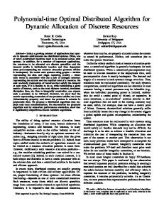
This equation is homogeneous, and so the solution is not unique. In other words, the solution can only be obtained to an unknown scale factor. However, if at least one edge length in the connected network is known, then the scale factor can be found to provide an unambiguous localization solution. IV. SIMULATION To assess its capability to support coordinated robotic flight, ANIM was simulated for a representative network of six robots, distributed in three-dimensions. Each robot was modeled as a node in the network, able to measure and communicate its unit pointing vectors to all other robots. Robot measurements were simulated at only a single time step, for the locations listed in TABLE I. All locations given in the table are listed in units of meters of displacement relative to the first robot (Node 1), designated to be at the origin. A total of 30 noisy measurements were simulated across the network, accounting for five measurements acquired by each of six robots. Measurement noise was simulated by adding a three-dimensional Gaussian random vector to the true measurement and scaling the vector sum back to unit length. The Gaussian random noise vector was modeled to be spherically symmetric. Its standard deviation in any direction was set to one of two values: either = 0.02 (2% of unit vector) or = 0.10 (10% of unit vector). ANIM converges quickly, with residual errors dropping by two orders of magnitude within 10 first-stage iterations. The results of the solution are shown in Fig. 2 ( = 0.02) and Fig. 3 ( = 0.10). True locations are represented as blue circles; ANIM estimates for 20 Monte Carlo trials are shown as red dots. The scale ambiguity was not explicitly resolved; however, for purposes of visualization, estimated edge lengths were scaled for best consistency with the truth. Estimates are plotted from the point of view of Robot 1, showing the inferred location of all other robots. Errors tend to align with the pointing vector to each robot j (e.g. in the illustration, errors tend to align with the true pointing vectors u1 j from node 1 to each other node j). As such, a standard deviation over the sample population was calculated for errors projected in the pointing-vector direction. Standard deviations are listed on the plots in two forms, as a percentage of range (reflecting the scale-factor ambiguity) and, for intuitive clarity, in units of meters (given consistency-based scaling). Not surprisingly, absolute errors (in meters) are largest for robots on the periphery, as the bearing measurements toward these robots are all acquired from roughly the same direction. Interestingly, percentage errors are larger nearest the reference node (Node 1) since, apparently, dividing by a short baseline magnifies the relative error.
ij
computed for any triangle by substituting (3) into (5) to give:
u12
u 23
d12 u31 d 23 0 . d31
TABLE I.
X (m) Y (m) Z (m)
NODE LOCATIONS RELATIVE TO ORIGIN (NODE 1)
Node 2 0 0 100
Node 3 300 -100 0
Node 4 -400 400 100
Node 5 -200 -200 200
Node 6 400 100 600
the future. Note that only the iterative part of the algorithm (Stage 1) was evaluated in a distributed manner. For the simulations presented, the distance estimates dij were computed in a centralized fashion. Future work is needed to de-centralize this processing stage, applying well understood principles for distributed solution of systems of linear equations [14].
700 13.38 m (1.8 %)
600 500
Z (m)
400 300
VI. SUMMARY
200
10.66 m (1.9 %)
100
7.33 m (2.1 %)
0
4.30 m (4.3 %) 6.57 m (2.1 %)
-100 500 0 -500
Y (m)
500
0
-500 X (m)
Fig. 2. ANIM results for 20 Monte Carlo trials ( = 0.02) 800
600
67.28 m (9.2 %)
REFERENCES [1]
Z (m)
400
200 35.37 m (10.2 %) 19.25 m (19.2 %)
53.12 m (9.2 %)
0
[2] [3]
44.59 m (14.1 %)
-200
[4]
1000 0
Y (m)
This paper presented ANIM, a novel localization method for processing angular measurements to obtain the relative 3D positions of a network of collaborating robots. The localization solution is subject to a scale-factor ambiguity, which can be resolved if at least one distance measurement relating node pairs is available. The proposed method is intended to leverage pre-existing robot equipment (e.g. communication systems), so that no additional weight or volume is required to install the navigation sensor. The algorithm inherently leverages distributed computation, which helps minimize communication and processing requirements for individual robots. Preliminary simulations suggest that ANIM consistently converges and provides reasonable accuracy, with localization errors about 2% of separation distance for 1.5 measurement errors.
-1000
[5] -600
-400
-200
0
200
400
600
X (m)
[6]
Fig. 3. ANIM results for 20 Monte Carlo trials ( = 0.10)
V. DISCUSSION The simulation provides preliminary guidance for design of a collaborative navigation system. Simulations suggest that relative position estimates with accuracy of about 2% of range (approximately 10 m on the scale of the simulation) are expected for the lower magnitude of measurement error ( = 0.02), which corresponds to an angular measurement error of about 1.5 accuracy. For the larger level of angular measurement error ( = 0.10, or about 5.7), position accuracy is insufficient for most robotic flight applications. Significant improvements to ANIM positioning accuracy are anticipated when the number of collaborating robots is increased. Testing this hypothesis will be an important topic for future work. Another important topic will be resolving the scale factor ambiguity by adding anchors or additional measurements. A key result was that ANIM functioned successfully as an iterative algorithm, converging in 100% of trials tested. This preliminary result provides confidence that the algorithm is likely to perform robustly when implemented in hardware in
[7]
[8]
[9] [10] [11] [12]
[13]
[14]
P. Misra and P. Enge, Global Positioning System: Signals, Measurements and Performance, Revised 2nd Ed., Ganga-Jamuna Press, Lincoln, MA, 2011. G. Siouris. Aerospace Avionics Systems: A Modern Synthesis, San Diego, CA: Academic Press, Inc 1993. Q. Lindsey, D. Mellinger, and V. Kumar, “Construction with quadrotor teams,” Autonomous Robots, Vol. 33, No. 3, pp. 323-336, 2012. Williamson, W., Rios, T., and Speyer, J., “Carrier Phase Differential GPS/INS Positioning for Formation Flight,” American Control Conference (ACC), San Diego, CA, 1999. John A. Volpe National Transportation Systems Center, “Vulnerability Assessment of the Transportation Infrastructure Relying on the Global Positioning System,” 29 Aug. 2001. Nishino, H., Tateishi, K., Ikegami, T., “Inter-Satellite Location Measurement of the Formation Flight Satellite System using UWB signal,” AIAA International Communications Satellite Systems Conference, AIAA, Seoul, South Korea, 2007. Chen, T., and Xu, S., “Approach Guidance with Double-Line-of-SightMeasuring Navigation Constraint for Autonomous Rendezvous,” Journal of Guidance, Control, and Dynamics, Vol. 34, No. 3, 2011, pp. 678-687. P. Biswas, H. Aghajan, and Y. Ye, “Semidefinite programming for sensor network localization using angle information,” Proc. IEEE 39th Asilomar Conf. Signals Systems and Computers, 2005. J. Rife, “Collaborative positioning for formation flight,” AIAA J. Guidance, Control, and Dynamics, vol. 46, no. 1, pp. 304-307, 2013. P. Mitiguy, Advanced Dynamics and Motion Simulation, MotionGenesis, 2013. E. Trucco and A. Verri, Introductory Techniques for 3-D Computer Vision, Prentice Hall, 1998. K. Doğançay and G. Ibal, “Instrumental variable estimator for 3D bearings-only emitter location,” IEEE Int. Conf. Intelligent Sensors, Sensor Networks and Information Processing, 2005. P. Biswas and Y. Ye, “Semidefinite programming for ad hoc wireless networking localization,” Proc. Int. Symp. Information Processing in Sensor Networks, 2004. U. Khan and J. Moura, “Distributing the Kalman Filter for large-scale systems,” IEEE Trans. Signal Processing, vol. 56, no. 10, pp. 49194935, 2008.