1856
IEEE TRANSACTIONS ON MEDICAL IMAGING, VOL. 35, NO. 8, AUGUST 2016
Deep Learning Guided Partitioned Shape Model for Anterior Visual Pathway Segmentation Awais Mansoor*, Juan J. Cerrolaza, Rabia Idrees, Elijah Biggs, Mohammad A. Alsharid, Robert A. Avery, and Marius George Linguraru
Abstract—Analysis of cranial nerve systems, such as the anterior visual pathway (AVP), from MRI sequences is challenging due to their thin long architecture, structural variations along the path, and low contrast with adjacent anatomic structures. Segmentation of a pathologic AVP (e.g., with low-grade gliomas) poses additional challenges. In this work, we propose a fully automated partitioned shape model segmentation mechanism for AVP steered by multiple MRI sequences and deep learning features. Employing deep learning feature representation, this framework presents a joint partitioned statistical shape model able to deal with healthy and pathological AVP. The deep learning assistance is particularly useful in the poor contrast regions, such as optic tracts and pathological areas. Our main contributions are: 1) a fast and robust shape localization method using conditional space deep learning, 2) a volumetric multiscale curvelet transform-based intensity normalization method for robust statistical model, and 3) optimally partitioned statistical shape and appearance models based on regional shape variations for greater local flexibility. Our method was evaluated on MRI sequences obtained from 165 pediatric subjects. A mean Dice similarity coefficient of 0.779 was obtained for the segmentation of the entire AVP (optic nerve only ) using the leave-one-out validation. Results demonstrated that the proposed localized shape and sparse appearance-based learning approach significantly outperforms current state-of-the-art segmentation approaches and is as robust as the manual segmentation. Index Terms—Anterior visual pathway, intensity normalization, MRI, partitioned statistical model, shape model, sparse learning.
I. INTRODUCTION HE anterior visual pathway (AVP) (Fig. 1) is responsible for transmitting all visual signals from retina to the brain. AVP consists of (a) a paired optic nerve also known as the cranial nerve II (CNII), (b) the optic chiasm: the part of AVP where nearly half of the fibers from each optic nerve pairs cross to the contralateral side, and (c) an optic tract pair. Optic tracts
T
Manuscript received January 01, 2016; revised February 12, 2016; accepted February 17, 2016. Date of publication February 26, 2016; date of current version July 29, 2016. This project was supported in part by a grant from the Gilbert Family Neurofibromatosis Institute and a philanthropic gift from the Government of Abu Dhabi to Children's National Health System . Asterisk indicates corresponding author. *A. Mansoor is with the Children's National Health System, Washington DC 20010 USA (e-mail:
[email protected]). J. J. Cerrolaza, E. Biggs, R. A. Avery, and M. G. Linguraru are with the Children's National Health System, Washington DC 20010 USA. R. Idrees is with the School of Medicine and Health Sciences, George Washington University, Washington DC 20052 USA. M. A. Alsharid is with the Department of Computer Science, Khalifa University, Sharjah, UAE . Color versions of one or more of the figures in this paper are available online at http://ieeexplore.ieee.org. Digital Object Identifier 10.1109/TMI.2016.2535222
Fig. 1. Schematic renderings of anterior visual pathway (AVP). Rendering of AVPs from different cohorts. Left to right: healthy control, subject with confirmed NF1 but no glioma, subject without NF1 with glioma behind the globe, and a subject having NF1 with gliomas throughout the distal optic nerves, chiasm, and optic tracts.
relay the information from the optic chiasm to the ipsilateral lateral geniculate nucleus, pretectal nuclei, suprachiasmatic nucleus, and superior colliculus. MRI sequences are widely used to non-invasively study and characterize diseases of AVP such as optic neuritis, optic nerve hypoplasia, and optic pathway glioma (OPG) [1]. OPGs are a low-grade tumors that occurs at any location along the AVP. In children with Neurofibromatosis type 1 (NF1), a genetic disorder of the nervous system, OPGs can be located in one or both optic nerves or throughout the entire AVP. In children with sporadic OPGs (i.e., not secondary to NF1), the tumor location is either restricted to one optic nerve or it encases the optic chiasm. OPGs may cause proptosis, strabismus, or vision loss. The natural history of these tumors, regardless of treatment, can demonstrate variable stages of growth or regression at any point along the AVP. Fig. 1 shows examples of AVP of healthy controls, patient with NF1 but without an OPG, sporadic OPG (i.e., not related to NF1) and patient with NF1 and an OPG. Recently, we proposed a quantitative metric for the detection of OPG in NF1 patients using T1-weighted MRI sequences [2]. The metric involves non-invasive quantification of the AVP including volume and diameter of the optic nerves, optic chiasm, and optic nerves from T1-weighted MRI sequences in healthy controls and subjects with OPG. The proposed metric showed promising results in the early detection and longitudinal tracking of tumors in OPG patients. However, the effective translation of the metric into clinical practice requires a robust automated segmentation method of the AVP, since it is impractical to perform time-intensive manual segmentation of morphologically complex structures. Moreover, the size and the appearance of AVP make accurate manual delineation much harder than manual segmentation of larger organs. To provide a perspective to the readers, in the current study we observed an inter-observer disagreement of about 20% for the
0278-0062 © 2016 IEEE. Personal use is permitted, but republication/redistribution requires IEEE permission. See http://www.ieee.org/publications_standards/publications/rights/index.html for more information.
MANSOOR et al.: DEEP LEARNING GUIDED PARTITIONED SHAPE MODEL FOR ANTERIOR VISUAL PATHWAY SEGMENTATION
Fig. 2. A typical axial plane view of MRI scan showing anterior visual pathway region. (a) Contrast-enhanced T1-weighted MRI sequence, (b) fat-saturated T2-weighted MRI sequence, (c) FLAIR MRI sequence. The optic nerves are pointed with red arrows and the optic chiasm with green.
AVP segmentation (Fig. 6), compared to 2–3% disagreement for organs such as lungs [3]. Fig. 2 shows a typical axial plane view of a typical AVP in T1-weighted, T2-weighted, and FLAIR MRI sequences. Automated segmentation of AVP from MRI is challenging due to their thin-long shape, poor contrast, and lack of sufficient discriminative features with the neighboring tissues [4]. A few automated segmentation methods from volumetric images have been previously reported in the literature with modest success. For instance, Bekes et al. [5] proposed a semi-automated approach using a geometrical shape model for the segmentation of optic nerves and eyeballs from computed tomography (CT) scans. The approach's reproducibility was found to be less than 50%. Noble et al. [6] presented a hybrid approach using a deformable model with a level set method to segment optic nerves and chiasm from CT/T1-weighted MRI pair. The method, tested on 10 healthy subjects, was reported to obtain a mean Dice similarity coefficient (DSC) of 0.8; however, in routine clinical practice CT and MRI are seldom acquired together for the same patient. Harrigana et al. [7] proposed another multi-atlas approach for the automated segmentation of optic nerves, muscles, and eye globes from volumetric CT data. They obtained an overall DSC of 0.77 using manual ground truth labels obtained from 30 healthy optic nerves. Panda et al. [8] extended Harrigana's approach for optic nerve segmentation from T2-weighted MRI sequences. The approach was tested on 4 subjects (1 healthy control, 1 multiple sclerosis patient, and 2 patients of optic head drusen), obtaining DSCs of 0.72, 0.76, and 0.61, respectively, for the pair of optic nerves. More recently, Dolz et al. [9] presented a fully automated method for the segmentation of the optic nerve pair using the support vector machine classification in 2D slices. A mean DSC of 0.76 was reported based on the testing performed on 10 healthy subjects. Most previous works were focused on the segmentation of one region of the AVP (i.e., optic nerve) with one exception by Yang et al. [10]. They developed a partitioned shape model approach for healthy AVP segmentation from T1-weighted MRI sequences by dividing the AVP into various shape homogenous segments and modeling each segment independently. To the best of our knowledge, this approach was the first attempt to accommodate local shape and appearance variation for AVP segmentation, reporting a DSC of 0.73 on 17 healthy AVP cases. None of the previously reported automated approaches have attempted to analyze chronic structural pathology of
1857
the AVP, such as an OPG. Depending on their severity, pathologies can have a dramatically different local shape and appearance characteristics than healthy cases, thus failing the shape model based segmentation methods. The challenge of segmenting larger anatomical structures with pathologies has been addressed numerously in the literature [3], [11]. However, the development of similar approaches for smaller vascular structures, such as the AVP, have traditionally been ignored. Recently, we presented, PAScAL (PArtitioned Shape and Appearance Learning) [12], a partitioned statistical shape model with sparse appearance learning method to segment both healthy and pathological AVP cases. In this work, we extended and improved PAScAL by incorporating complementary information from multi-sequence MRIs and adding new methodological features. The main contributions of this work are: (1) a fast marginal space deep learning approach for an accurate initialization of the statistical shape models; (2) a 3D multiscale intensity normalization method of volumetric medical image by energy standardization of curvelet subbands, (3) a partitioned appearance model that combines the complimentary information from T1-weighted, fat-saturated T2-weighted, and FLAIR MRI sequences to characterize regions with subtle differences in appearance from the neighboring tissues; and (4) a comprehensive evaluation performed on 165 healthy and pathological cases. (5) Last, but not the least, a deep learning paradigm is proposed by applying stacked autoencoder (SAE) to learn deep learning feature representation from the MRI sequences for steering the shape model in AVP segmentation, particularly useful in the cases with structural pathologies. The paper is organized as follows. Section II provides a brief background on the SAE. Section III introduces our deep network guided partitioned statistical model. Experimental results are presented in Section IV followed by discussion and conclusions. II. BACKGROUND A. Hierarchical Deep Feature Learning Architecture Using the Stacked Autoencoder Recently, unsupervised deep learning has gained a lot of interest as robust discriminative feature representation especially in the characterization of brain tissues from MRI sequences [13], [14]. A deep learning paradigm begins by learning low-level features and hierarchically building up comprehensive high-level features in a layer-by-layer manner. In our framework we used deep learning representation to infer the feature representation from MRI sequences for (i) the localization of AVP, and (ii) the creation of the appearance models to capture local appearance characteristics of the AVP. An SAE is a deep neural network consisting of multiple layered sparse autoencoders (AE) in which the output of every layer is wired to the input of the successive layer. Specifically, the output of a low-level AE (AE trained on low-level features) is the input of high-level AE. An AE consists of two components: the encoder and the decoder. The encoder aims to fit a non-linear mapping that can project higher-dimensional observed data into its lower dimension feature representation.
1858
IEEE TRANSACTIONS ON MEDICAL IMAGING, VOL. 35, NO. 8, AUGUST 2016
Fig. 3. Overview flow diagram of PAScAL.
TABLE I DESCRIPTION OF THE DATA USED IN OUR EXPERIMENTS.
Snap interactive software application (http://www.itksnap.org/) and the T1-weighted MRI sequences under the supervision of an expert neuro-ophthalmologist. C. Pre-Processing
The decoder aims at recovering the observed data from the feature representation with minimal recovery error. For a detailed description of AE, SAE, and related deep learning concepts, reader is encouraged to review [15], [16]. III. METHODS A. Overview The PAScAL framework presented in this manuscript, automatically segments the AVP using the joint partitioned shape models steered by an appearance model that is created using a combination of T1-, T2-, and FLAIR-weighted MRI sequences along with deep-learning features. In order to create a generic cross-platform solution that can work with images collected from multiple sources, a multiscale normalization method is proposed, using the 3D curvelet transform, as a pre-processing step for the intensity standardization of the test data to the reference range. Our method adapts the classical statistical models for thin tubular structure by introducing a partitioned shape modeling approach for shape flexibility and robust appearance learning. Like most model and training-based methods, our segmentation approach consists of training and testing modules. The flow diagram shown in Fig. 3 provides an overview of the method. The following sections present in detail each methodological step. B. Data and Reference Standards After the Institutional Review Board approval, Gadolinium (Gd) contrast-enhanced T1, fat-saturated T2, and Fluid-attenuated inversion recovery (FLAIR) MRI scans were acquired from 165 patients. The acquisition and demographic details of the patients are provided in Table I. The dataset was anonymized during the image retrieval. The ground truth segmentation was prepared manually by two experienced raters using the ITK-
1) Conditional Sparse Space Deep Learning Localization: Statistical shape models are sensitive to initialization [17]. Initialization far from the target boundary could potentially compromise the performance of even the best-crafted models. Lately, a number of techniques for robust model initialization for large organs have been presented [18], [19]; however, the issue of automated initialization for smaller structures has not been amicably addressed. Robust shape model initialization for smaller structures with poor and variable image contrast such as the AVP is especially challenging. In this work, we introduced an unsupervised feature representation approach for the localization of objects in volumetric image data employing the conditional space deep learning architecture. Our approach works by gradually eliminating regions with lower probability of being the target organ. Specifically, the object to be localized is modeled using a bounding box centered at a voxel . Subsequently, the object localization problem is transformed into a machine classification problem to detect if a given voxel in the test image is the centroid of the object of interest or not. Specifically, we aim at finding that maximizes the posterior probability over the entire space, i.e., (1) Due to the exponential number of the hypotheses, an exhaustive search of the target object using (1) is impractical. Instead we extend the marginal space deep learning approach proposed in [20] for AVP localization. We begin by splitting the parameter space into marginal subspaces as the concatenation of marginal probabilities: (2) The space learning method provides an efficient run-time solution by learning classifiers in higher-dimensional space features in the regions with higher marginal probability only. To further expedite the space learning paradigm, instead of using the volumetric data directly for learning, we learn the deep-learning classifier on a 2D depth projection image extracted from a 3D
MANSOOR et al.: DEEP LEARNING GUIDED PARTITIONED SHAPE MODEL FOR ANTERIOR VISUAL PATHWAY SEGMENTATION
Fig. 4. The pipeline for anterior pathway localization.
volume patch . The approach is motivated by the view-based 3D shape techniques presented in [21], [22]. Specifically, for a 3D volume centered at point , in order to localize the object along a plane , we collect the 2D projection set from centered at along plane . In our study we used minimum intensity projection (MinIP) [23] for AVP localization (i.e., ). The posterior probability in (1) and (2) can therefore be rewritten in terms of 2D projections as: (3) The superscript T1 indicates the projections for localization were extracted from T1-weighted sequences only. In our study, we used isotropic volumetric patches of size voxels to produce the projection image. The size of volumetric patch was estimated empirically as the largest bounding box enclosing the manually segmented ground truth within the entire dataset. In addition, the bounding box is aligned to the volume axes; therefore, no orientation estimation was necessary. Given a 2D projection , the classification problem for the location estimation was formulated as whether the center of the object of interest (AVP) along the plane was located at the location . A positive sample should satisfy voxel, where denotes the position of the bounding-box enclosing the manually segmented ground truth of the AVP along the plane . Then, we applied the SAE classifier to to inferring the deep-learning feature representation. For AVP localization, three hidden layers were employed in the SAE framework. The number of units in each SAE layer was 400, 200, and 100 respectively. The target activation for hidden units was set to 0.15, the sparsity penalty was set to 0.1, and the batch size was 100. The number of epochs used was 100. The trained SAE classifier was used to calculate the probability for every voxel in the test image being the centroid of AVP. A small number of candidates (100 in our experiments) having the highest probability of being the centroid of AVP were propagated to the next stage where the same deep-learning classification procedure was repeated for the next plane. The final position of the bounding box enclosing the AVP was estimated by the majority voting of the 100 highest probability candidates after the third plane. The proposed localization method is summarized in Fig. 4. Using the approach, a speed enhancement of up to 15 times in AVP localization was observed compared to an exhaustive search ((1)). Due to relatively high and almost anisotropic resolution of T1 scans in our dataset, the order of the planes within the localization module did not affect the performance in our experiments; however, the efficiency for images acquired under highly anisotropic resolution settings may be subject to the ordering of
1859
planes. Also, the minimum intensity projection, adopted to expedite the localization process, assumes that the AVP (especially the optic nerve region) is generally darker than the neighboring tissues in the T1-weighted MRI [4]. This assumption may not hold true universally for other objects of interest or acquisition settings, for instance, maximum intensity projection (MaxIP) instead of MinIP was found to be more appropriate in localizing the AVP from T2-weighted sequences since AVP appears brighter than the neighboring tissues in T2 weighted scans. 2) Multiscale 3D Curvelet-Based Intensity Normalization: Unlike in CT scans that have standard intensity values due to the adaptation of Hounsfield units, the appearance characteristics of MRI sequences are influenced by acquisition settings, scanner technology, and proprietary reconstruction algorithms. Many computer-aided diagnosis approaches perform sub-optimally when test data statistics do not resemble closely with the training data. Intensity normalization (or standardization) can help to modify the characteristics of test data to resemble closely to training data. Commonly used approaches to intensity normalization include linear rescaling, histogram matching, and histogram equalization. However, the quantitative analysis of small objects with low image contrast such as the AVP, requires more elaborate and sophisticated normalization method. A few attempts have been made recently in the literature towards designing modality specific approaches to intensity normalization. For instance, Mirzaalian et al. [24] used spherical harmonics basis functions to estimate region specific linear mapping between diffusion MRI data collected at multiple sites and scanners. Philipsen et al. [25] presented a method for the intensity normalization of chest radiographs using localized energy bands. In this work, we propose a generic multiscale framework for the intensity normalization of volumetric images based on the localized energy standardization of 3D curvelet-transform subbands. The curvelet transform [26] is a high-dimensional generalization of the wavelet transform designed to represent objects at different scales and orientations. Unlike wavelets, the transform is not only localized in space and scale but also in orientation. Due to its strong anisotropic properties resulting from frequency localization at various scales, the curvelet transform has proven to be an efficient tool in various imaging applications such as denoising [26] and segmentation [27]. Our intensity normalization method exploits the frequency localization property of the curvelet transform by standardizing the local energies of individual subbands with respect to reference subbands. Once the centroid localizing the AVP within the image has been identified using the procedure outlined in Section III-C1, the intensity normalization module was initiated for bounding-box around the centroid only instead of the entire image. The strategy is computationally efficient and demonstrated better normalization for the AVP segmentation in our experiments. In the curvelet domain, the input image is decomposed into several subbands having a given scale and an orientation . A discrete curvelet transform of a function is a dyadic sequence of scale , orientation , and spatial location called curvelet coefficients defined by, , where is the 3D discrete
1860
IEEE TRANSACTIONS ON MEDICAL IMAGING, VOL. 35, NO. 8, AUGUST 2016
D. Shape Initialization Following the AVP localization and intensity normalization of the localized bounding box image , the AVP shape model is initialized at the centroid . To create and initialize the AVP shape model from MRI, the following steps were performed: 1) Landmark Extraction: For AVP shapes (manually annotated binary images), first the centers of mass of all shapes were aligned. Subsequently, landmarks at each of the training shapes were calculated using the marching cubes algorithm [28]. 2) Mean Shape Calculation: Each training shape consists of a set of annotated landmarks aligned through Procrustes analysis, i.e., , where denotes the column
curvelet transform and of an individual subband at scale defined as:
. The energy and orientation is
(4) is the 3D discrete curvelet subband, is the average value of curvelet coefficients within the subband, and is the number coefficients within the subband. During the training stage, reference energies for every subbands were calculated using , where (4) from the training scans is the number of scans in the training set (in our experiments for every MRI sequence (T1, T2, FLAIR)). During the testing stage, the normalized curvelet coefficients of the test data were determined using the reference energy values from the training stage: where
(5) is the ratio of reference subband energy to the test where subband energy and measures how close the energy of the test subband is to the reference band . In order to have an almost complete correspondence, the normalization procedure (described in (5)) was repeated iteratively for the reconstructed test image iteratively until . Algorithm 1 provides the pseudo-code for the proposed normalization method.
training shape vector of 3D coordinates of landmark in the . Let be the training shape after Procrustes analysis then the mean shape was calculated by averaging over the mean location of the landmarks across the training shapes from . Subsequently, principal component analysis (PCA) was used to compute the normalized eigenvectors and eigenvalues of the covariance matrix across the training shapes. Finally, a linear combination of eigenvectors was used to generate the initial shape model, , where is a matrix with the top eigenvectors (98% energy) describing the principal mode of variation in the training shapes, and is a vector of scaling values for the principal components. This type of PCA analysis is used by traditional shape models [29]. The PCA of the entire shape and the constraints on makes the traditional ASM less flexible for local shape variations. We addressed this shortcoming with a partitioned shape model, as described later in the paper (Section III-F). However, to create robust partitions, we must rank the landmarks in the training data based on their strength in segmenting the AVP from the neighboring tissues as described in the following subsection. E. Multi-Sequence Landmark Weighting As discussed previously, various regions of the AVP have varying degrees of appearance contrast. In our experiments, the optic tract region of the AVP was found to have the greatest inter-observer variability due to varying contrast, making it hard to reliably define boundaries in the region even manually. Therefore, the landmarks belonging to the tract region may not be as reliable as the ones in the nerve region that showed a stable contrast with the neighboring tissues. In this work, we used the concept of landmark weighting based on their stability. The proposed weighting ranks landmarks based on the variability of appearance profile. To calculate weights, the intensity profile of size around each landmark in every appearance channel (T1, T2, FLAIR, SAE) was first extracted and stacked together. For each landmark , the covariance matrix of appearance profile across the training data was calculated. A landmark is considered “stable” if it demonstrated lower variance (similar appearance characteristics). Subsequently, the weight of landmark is calculated as: (6) where
denotes the trace of the matrix.
MANSOOR et al.: DEEP LEARNING GUIDED PARTITIONED SHAPE MODEL FOR ANTERIOR VISUAL PATHWAY SEGMENTATION
F. Landmark Partitioning In order to adapt the statistical shape model to the tubular AVP, the landmarks were divided into various partitions having consistent local shape and appearance variation. Since the AVP is a tubular structure, the resulting individual partitions should maintain this characteristic. To group landmarks into clusters and to make the adjacent partitions overlap for smoother boundary transition amongst the partitions, we employ affinity propagation clustering [30]. The deformable training shape was decomposed into partitioned shapes with each partition consisting of landmarks. In order to ensure that a certain partition did not contain only the “unstable” landmarks, the average landmark weight of each partition was also calculated. If the average weight of a partition was below a certain threshold , then it was merged with its immediate neighbor towards the chiasm. The details of the proposed partitioning method are presented in Algorithm 2. G. Partitioned Statistical Shape Model In the traditional shape models, shape parameters are represented in the hyperspace defined by eigenvectors. For our partitioned hyperspaces, we used the hierarchical shape model proposed by fitting a second order PCA to partitioned training shapes in the new combined hyperspace . The individual shape partition where is the partition index, is the shape vector and is the mean shape vector corresponding to partition . is the combined shape vector of all partitions combining all shape parameters of different partitions and is eigenvectors matrix. is the matrix of eigenvectors of the shape in the hyperspace and is the global scaling vector of the entire training shape to ensure that the deformable shape formed by joining different partitions stays within the training shape constraints. During the model fitting, the shape vector for every partition was updated iteratively until convergence. The scaling vector for partition
1861
was calculated using the landmark weighting paradigm proposed in Section III-E. Using the method outlined in [31], the shape parameters for partition was determined based on the appearance profile weighted landmarks. (7) where is the diagonal matrix containing the weights of landmarks in partition . In order to ensure that the adjacent partitions have smooth connectivity during model fitting, overlapping regions between partitions were introduced; thus overlapping landmarks appear in multiple partitions. During model fitting, the shape parameters for individual partitions were calculated separately and the shape parameters of the overlapping landmarks were computed using the mean of the shape parameters from the multiple partitions they belong. H. Multi-Sequence Deep Learning Features Steered AVP Segmentation Our proposed segmentation framework is based on the ASM method originally presented by Cootes et al. [29] and follows an iterative approach where the location of each landmark was updated based on a specific appearance model (i.e., minimizing an energy function that combines the probability map of the AVP class obtained using the SAE architecture and additional intensity information from T1, T2, and FLAIR sequences). The SAE probability map for AVP was obtained for the localized region of test image by applying the SAE classifier trained using T1, T2, and FLAIR sequences and manually annotated ground truth. During the testing stage, given the MRI sequences (T1, T2, and FLAIR) and an initial AVP shape , the method begins by localizing the AVP (Section III-C1), followed by the intensity normalization of all MRI sequences within the localized region (Section III-C2) followed by SAE probability map creation. Finally, local shape models constructed for different par-
1862
IEEE TRANSACTIONS ON MEDICAL IMAGING, VOL. 35, NO. 8, AUGUST 2016
TABLE II FOR ACTIVE SHAPE MODELS. VALUES IN OUR EXPERIMENTS ARE PROVIDED.
PARAMETERS
USED
Fig. 5. Shape and appearance consistent clustering of the AVP landmarks. (leftto-right) The AVP clustered into 3, 13, and 23 partitions using Algorithm 2 are shown.
titions in the training stage (Section III-G) were used to guide the deformation of the initial shape individually. This deformation guided by the local appearance models (Section III-H) was iteratively performed till convergence. The parameters of our partitioned ASM segmentation scheme are listed in Table II. We follow the description and notation of [32]. IV. EXPERIMENTAL RESULTS A. Inter-Observer Agreements and the PAScAL Performance To quantify the performance of PAScAL with manually created ground-truths by experts, the DSC of the manually delineated AVP labels and our multi-sequence approach, PAScAL, were computed. Fig. 6 shows the box-plots of DSC inter-observer agreements and PAScAL. Based on evaluation of the PAScAL framework on MRI sequences obtained from 165 pediatric subjects, the performance of PAScAL was found to be within the limits of inter-observer disagreement. An average DSC of is obtained for manual segmentation and for PAScAL (p-value ). B. Performance Analysis of Individual Modules 1) Effect of Intensity Normalization: Fig. 7(a) shows the landmark-to-surface of PAScAL with and without the intensity normalization of images. For comparison purposes, the performance was analyzed on the dataset without standardization, baseline standardization method of linear rescaling, the histogram equalization, after applying intensity normalization using the method proposed in Section III-C2. For the linear-rescaling, the intensity values were linearly rescaled to zero mean and unit variance. The histogram equalization and linear-rescaling was performed within the localized region only. An average landmark-to-surface distance of was observed with proposed intensity nor-
Fig. 6. Box-plots of Dice similarity coefficient for inter-observer agreement ). and PAScAL (p-value
malization method as opposed to (p-value ) with linear rescaling, (p-value ) using histogram equalization, and (p-value ) without normalization. The performance of global intensity normalization was found to be worse. 2) Effect of Using Multi-Sequence MRI and Deep Networks Architecture: Fig. 7(b) presents the mean landmark-to-surface distance of the AVP segmentation framework, PAScAL, for employing intensity values from a single MRI sequence (T1), multiple MRI sequences, and multiple MRI sequences with hand-crafted Haar-like features [33], and the deep learned (SAE) features. An average landmark-to-surface distance of (p-value ) was obtained with T1-weighted sequences only, (p-value ) with T1-weighted, T2-weighted, and FLAIR MRI sequences, (p-value ) with hand-crafted Haar-like features, and for MRI sequences with SAE features. The parameters of the SAE framework used in our experiments are provided in Section IV-B4. The use of multiple sequences with deep learned features demonstrated significant improvements over using just the T1-weighted sequence (p-value ), the MRI sequences only (p-value ), and the hand-crafted Haar-like features (p-value ), as, determined by the Wilkcoxon rank sum test. Significant improvement in performance was also observed by using multi-sequence MRI over using T1-weighted sequence only (p-value ). 3) Effect of Number of Partitions: Fig. 8 shows the segmentation performance of PAScAL in terms of mean landmark-to-
MANSOOR et al.: DEEP LEARNING GUIDED PARTITIONED SHAPE MODEL FOR ANTERIOR VISUAL PATHWAY SEGMENTATION
1863
Fig. 7. (a) The mean landmark-to-surface distance without intensity normalization and with intensity normalization using the linear-rescaling, histogram equalization, and the proposed normalization method. (b) The mean landmark-to-surface distance using box-plots for T1 only, multiple MRI sequences, hand-crafted Haar-like features, and SAE features. (c) Box-plots comparing the mean landmark-to-surface distance map of AVP using different deep-learning architectures. (d) Mean landmark-to-surface distance map of AVP using different AVP segmentation approaches is reported using box-plots.
Fig. 8. Effect of the number of partitions on the performance accuracy of AVP segmentation. Mean landmark-to-surface distance map of AVP using different partition schemes is shown (a)-(c). (d) Average landmark error for using different number of partitions is presented. (a) 7-partitions (b) 22-partitions (c) 52-partitions (d).
surface distance using different partition strategies. The performance showed a significant improvement initially with an increase in the number of partitions. However, the performance did not improve when more than 22 partitions were created, due primarily to the loss of contextual neighborhood information. In our experiments, an average improvement of 0.415 mm per landmark was observed from 6 partitions to 22 partitions (p-value ); however, the average distance per landmark increased by 0.0282 mm when the number of partitions were increased from 22 to 32 (p-value=0.061). Based on these empirical data, we used 22 partitions for our experiments. 4) Effect of Deep Learning Architectures: To compare the effect of different deep architectures, we compared two well-known unsupervised deep learning algorithms, namely, the stacked autoencoder (SAE) and deep belief networks (DBN). DBN are generative neural network models introduced by Hinton et al. [34]. The building block of a DBN is the probabilistic model known as Restricted Boltzman machine. Both SAE and DBN involve learning a model of the training data distribution. To steer partitioned shape models for AVP segmentation in the PAScAL framework, the similarity map of the AVP class, obtained using the deep-learning architecture, was used as one of the appearance feature. To compare different deep learning strategies, we tried both SAE and DBN frameworks. For SAE framework, three hidden layers were employed. The number of units in each SAE layers was 400, 200, and 100, respectively. The target activation for hidden units was set to 0.15, the sparsity penalty was set to 0.1, the
batch size was set to 100, and the stochastic gradient descent (SGD) optimization with Nesterov momentum coefficient of 0.5. The number of epochs used was 100. Similarly, for training the DBN we used 100 hidden Restricted Boltzmann machine (RBM) units, three hidden layers , and a batch size of 100. Fig. 7(c) shows the box plots of average landmark-to-surface distance using the SAE and DBN deep learning architectures. In our experiments, SAE outperformed DBN (average landmark error and respectively, Wilkcoxon rank sum test (p-value ). Moreover, our experiments were consistent with other reports in the literature that suggested that autoencoders are generally faster and easier to train than the deep networks [35]. C. Performance Analysis of the Entire Framework (PAScAL) 1) Comparison With Current State-of-the-Art Methods on the Same Dataset: In order to provide a comparison of the performance of different methods, we performed additional experiments using two shape-based methods on our dataset, namely, the classic active shape model (ASM) [29] and Yang et al.'s method for AVP segmentation [10]. The classical ASM was tested with the same configuration as our method, except that shape partitioning was not performed and the normalized derivative profiles were used as proposed in the classical ASM in place of the SAE features. Yang's method was executed using the settings reported in their paper. The comparative performance of three methods is reported in Fig. 7(d). Average error per landmark obtained was for ASM,
1864
IEEE TRANSACTIONS ON MEDICAL IMAGING, VOL. 35, NO. 8, AUGUST 2016
TABLE III OF THE STATE-OF-THE-ART METHODS REPORTED IN THE LITERATURE FOR AVP SEGMENTATION.
SUMMARY
for Yang et al. (p-value , compared to ASM) and for PAScAL (p-value , compared to Yang's method). All components and parameters were kept the same for the experiments performed with ASM. The highest 98% eigenvectors were preserved in all the compared methods. AVPs, especially the ones suffering from a genetic disorders like NF1, result in nerve tortuosity [36] (as shown in Fig. 1). From our observations, the global modeling of ASM did not accommodate well local shape variations, such as tortuosity. Moreover, changes in AVP shape can occur at random locations and since the AVP is only a few voxels wide, these local shape accommodations make a great difference in the overall accuracy. The impact of local modeling in performance may be less significant in larger organs. 2) Comparison With Other Methods Reported in the Literature: For comparison of PAScAL with other methods presented in the literature, we compile the performance reported by current state-of-the-art methods in Table III. The table summarizes performance of different methods in terms of the size of data and DSC metric. Note that most methods did not segment the entire AVP. V. DISCUSSION In the design of any CAD application, the automated accurate segmentation of the organ (or tissue) of interest is the most important initial step. Automated Segmentation is particularly challenging for small structures, such as AVP. The AVP segmentation is difficult not only due to large variations of appearance, but also because of the high level of precision that is needed for clinical use. A recent study, [2], conducted by our group showed that the average volumetric differences between the healthy AVP and pathological cases with OPG is 0.15 ml on average. On a high resolution MRI scan with an average voxel size of , such as the ones used in this study, 0.15 ml translates to roughly only 2000 voxels (an average MRI scan has close to 8,000,000 voxels). Although significant progress has been made in the development of CAD tools for larger organs [3], [37], it is due to the aforementioned difficulties that the expert manual segmentation is still considered the best approach. However, due to large inter-observer variability and the amount of time required for manual segmentation, no universal quantitative criteria exists currently for the diagnosis of AVP pathologies. With PAScAL, we envisioned to expand our recent attempt [2] to establish a universal quantitative criteria for the detection and diagnosis of
AVP pathologies. Traditional statistical models, such as ASM [29], lack flexibility to model tubular structures such as AVP. PAScAL is aimed at providing that flexibility by localized shape partitioning. PAScAL was tested on MRI scans collected from 165 subjects with a wide demographic background and pathological condition (Table I). By testing our method on a versatile data, we made every effort possible to validate the performance of PAScAL. However, we believe that due to the fully automated nature of the method, additional pre-processing and/or post-processing steps may be needed for difficult or rare cases. The following discussion is designed to create better understanding of the method's performance. A. Excessive Noise PAScAL does not have a built-in denoising mechanism. The method, with the help of the intensity normalization module, can tolerate a wide range of intensity variations. However, it may struggle in the presence of excessive noise and rare appearance artifacts. Nevertheless, pertinent denoising mechanism may be readily integrated into the approach. B. Image Resolution In clinics, T2 and FLAIR sequences are often acquired at lower resolution than their T1 counterparts. During our validation studies, we tested PAScAL at lower resolution across various planes in T2 and FLAIR scans and the method was found to be robust to a wide range of resolution levels (see Table I for details). However, some loss of accuracy should be expected when lower resolution scans are used. C. Rare Clinical Cases A strength of PAScAL is the introduction of a partitioned statistical shape model-based framework that accommodates local shape variations. However, the model still follows the overall shape constraints of the AVP and in certain extreme cases where the glioma in the AVP fundamentally alters the shape of the AVP (rightmost case in Fig. 1, using PAScAL), PAScAL may struggle to accommodate the shape boundaries. Moreover, as the validation data in our study was not collected under a protocol designed specifically for the analysis of AVP, a study should be conducted to establish the optimal AVP protocol, including the MRI sequences to acquire, resolution ranges and pertinent acquisition parameters. Nevertheless, in its current form, PAScAL is a promising tool for the routine analysis and quantification of AVP-related disorders. VI. CONCLUSION Accurate delineation of the object of interest is the first step in any image-based quantification. Automated quantification of the anterior visual pathway (AVP) in MRI is challenging due to their thin small size, structural variation along the path, and non-discriminative contrast to the adjacent anatomic structures. In this paper, we presented a fully automated approach for the segmentation of AVP from MRI scans using deep learning features extracted from multi-sequence MRI. To the best of our knowledge, PAScAL is the first fully automated approach for the segmentation of AVP from MRI scans with and without pathology. PAScAL initiates with a robust shape localization
MANSOOR et al.: DEEP LEARNING GUIDED PARTITIONED SHAPE MODEL FOR ANTERIOR VISUAL PATHWAY SEGMENTATION
was proposed to set the shape model close to the AVP boundary using conditional deep learning space. Second, a curvelet transform-based intensity normalization module was created to construct appearance models that are robust across a wide variety of acquisition settings. Third, a partitioned statistical shape model was designed to enable regional shape variations in the anatomy including pathology. Finally, local appearance models were learned by adopting deep learning architecture to extract hierarchical features from multi-sequence MRI scans. PAScAL was tested on scans from 165 patients collected at our institution using multiple MRI scanners. Results demonstrated that PAScAL significantly outperformed other reports in the literature and achieves performance within the range of inter-observer variability. The robustness of PAScAL in segmenting AVP indicates the method's potential and generic applicability to anatomical structures sharing similar structural and appearance characteristics such as some of the other cranial and spinal nerves [38]. REFERENCES [1] J. Chan, Optic Nerve Disorders. New York: Springer, 2007. [2] A. Mansoor, R. Idrees, R. Packer, M. G. Linguraru, and R. A. Avery, “Automated MRI segmentation of the anterior visual pathway: Establishing quantitative criteria for OPG in children with NF1,” in Proc. NF Conf. Children's Tumor Found., 2015. [3] A. Mansoor et al., “A generic approach to pathological lung segmentation,” IEEE Trans. Med. Imag., vol. 33, no. 12, pp. 2293–2310, Dec. 2014. [4] S. Sheth, B. F. Branstetter IV, and E. J. Escott, “Appearance of normal cranial nerves on steady-state free precession MR images,” Radiographics, vol. 29, no. 4, pp. 1045–1055, 2009. [5] G. Bekes, E. Máté, L. G. Nyúl, A. Kuba, and M. Fidrich, “Geometrical model-based segmentation of the organs of sight on CT images,” Med. Phys., vol. 35, no. 2, pp. 735–743, 2008. [6] J. H. Noble and B. M. Dawant, “An atlas-navigated optimal medial axis and deformable model algorithm (NOMAD) for the segmentation of the optic nerves and chiasm in MR and CT images,” Med. Image Anal., vol. 15, no. 6, pp. 877–884, 2011. [7] S. Panda et al., “Robust optic nerve segmentation on clinically acquired CT,” Proc. SPIE Med. Imag., p. 90341G, 2014. [8] S. Panda, A. J. Asman, L. A. Mawn, B. A. Landman, and S. A. Smith, “Robust segmentation of clinical optic nerve MRI,” Int. Soc. Magn. Reson. Med., 2013. [9] J. Dolz, H. Leroy, N. Reyns, L. Massoptier, and M. Vermandel, “A fast and fully automated approach to segment optic nerves on MRI and its application to radiosurgery,” in Proc. IEEE Int. Symp. Biomed. Imag., From Nano to Macro, 2015, pp. 1102–1105. [10] X. Yang, J. Cerrolaza, C. Duan, Q. Zhao, J. Murnick, N. Safdar, R. Avery, and M. G. Linguraru, “Weighted partitioned active shape model for optic pathway segmentation in MRI,” in Clinical Image-Based Procedures. Translational Res. in Medical Imaging. New York: Springer, 2014, pp. 109–117. [11] A. Mansoor et al., “Segmentation and image analysis of abnormal lungs at CT: Current approaches, challenges, and future trends,” RadioGraphics, vol. 35, no. 4, pp. 1056–1076, 2015. [12] A. Mansoor, J. Cerrolaza, R. Avery, and M. G. Linguraru, “Partitioned shape modeling with on-the-fly sparse appearance learning for anterior visual pathway segmentation,” in Clinical Image-Based Procedures. Translational Res. in Medical Imaging. New York: Springer, 2015, pp. 109–117. [13] W. Zhang et al., “Deep convolutional neural networks for multi-modality isointense infant brain image segmentation,” NeuroImage, vol. 108, pp. 214–224, 2015. [14] S. M. Plis et al., “Deep learning for neuroimaging: A validation study,” Front. Neurosci., vol. 8, 2014.
1865
[15] Y. Bengio et al., “Greedy layer-wise training of deep networks,” Adv. Neural Inf. Process. Syst., vol. 19, p. 153, 2007. [16] H. Larochelle, D. Erhan, A. Courville, J. Bergstra, and Y. Bengio, “An empirical evaluation of deep architectures on problems with many factors of variation,” in Proc. 24th Int. Conf. Mach. Learn., 2007, pp. 473–480. [17] J. Liu and J. K. Udupa, “Oriented active shape models,” IEEE Trans. Med. Imag., vol. 28, no. 4, pp. 571–584, Apr. 2009. [18] F. A. Cosío, “Automatic initialization of an active shape model of the prostate,” Med. Image Anal., vol. 12, no. 4, pp. 469–483, 2008. [19] R. Toth et al., “A magnetic resonance spectroscopy driven initialization scheme for active shape model based prostate segmentation,” Med. Image Anal., vol. 15, no. 2, pp. 214–225, 2011. [20] Y. Zheng, A. Barbu, B. Georgescu, M. Scheuering, and D. Comaniciu, “Four-chamber heart modeling and automatic segmentation for 3D cardiac CT volumes using marginal space learning and steerable features,” IEEE Trans. Med. Imag., vol. 27, no. 11, pp. 1668–1681, Nov. 2008. [21] Z. Zhu, X. Wang, S. Bai, C. Yao, and X. Bai, “Deep learning representation using autoencoder for 3D shape retrieval,” in Proc. Int. Conf. IEEE Security, Pattern Anal., Cybern., 2014, pp. 279–284. [22] D.-Y. Chen, X.-P. Tian, Y.-T. Shen, and M. Ouhyoung, “On visual similarity based 3D model retrieval,” Comput. Graphics Forum, Wiley Online Library, vol. 22, no. 3, pp. 223–232, 2003. [23] D. D. Cody, “AAPM/RSNA physics tutorial for residents: Topics in CT,” RadioGraphics, vol. 22, no. 5, pp. 1255–1268, 2002. [24] H. Mirzaalian, A. de Pierrefeu, P. Savadjiev, O. Pasternak, S. Bouix, M. Kubicki, C.-F. Westin, M. E. Shenton, and Y. Rathi, “Harmonizing diffusion MRI data across multiple sites and scanners,” in Medical Image Computing and Comput.-Assisted Intervention-MICCAI 2015. New York: Springer, 2015, pp. 12–19. [25] R. Philipsen et al., “Localized energy-based normalization of medical images: Application to chest radiography,” IEEE Trans. Med. Imag., vol. 34, no. 9, pp. 1965–1975, Sep. 2015. [26] J.-L. Starck, E. J. Candès, and D. L. Donoho, “The curvelet transform for image denoising,” IEEE Trans. Image Process., vol. 11, no. 6, pp. 670–684, Jun. 2002. [27] J.-L. Starck, F. Murtagh, E. J. Candes, and D. L. Donoho, “Gray and color image contrast enhancement by the curvelet transform,” IEEE Trans. Image Process., vol. 12, no. 6, pp. 706–717, Jun. 2003. [28] W. E. Lorensen and H. E. Cline, “Marching cubes: A high resolution 3D surface construction algorithm,” ACM Siggraph Comput. Graph., vol. 21, no. 4, pp. 163–169, 1987. [29] T. F. Cootes, C. J. Taylor, D. H. Cooper, and J. Graham, “Active shape models-their training and application,” Comput. Vis. Image Understanding., vol. 61, no. 1, pp. 38–59, 1995. [30] B. J. Frey and D. Dueck, “Clustering by passing messages between data points,” Science, vol. 315, no. 5814, pp. 972–976, 2007. [31] M. Zhao, S. Z. Li, C. Chen, and J. Bu, “Shape evaluation for weighted active shape models,” in Proc. Asian Conf. Comput. Vis., 2004, pp. 1074–1079. [32] B. Van Ginneken et al., “Active shape model segmentation with optimal features,” IEEE Trans. Med. Imag., vol. 21, no. 8, pp. 924–933, Aug. 2002. [33] M. Villamizar, A. Sanfeliu, and J. Andrade-Cetto, “Computation of rotation local invariant features using the integral image for real time object detection,” in Proc. 18th Int. Conf., IEEE Pattern Recognit., 2006, vol. 4, pp. 81–85. [34] G. E. Hinton, S. Osindero, and Y.-W. Teh, “A fast learning algorithm for deep belief nets,” Neural Comput., vol. 18, no. 7, pp. 1527–1554, 2006. [35] P. Vincent, H. Larochelle, I. Lajoie, Y. Bengio, and P.-A. Manzagol, “Stacked denoising autoencoders: Learning useful representations in a deep network with a local denoising criterion,” J. Mach. Learn. Res., vol. 11, pp. 3371–3408, 2010. [36] J. Ji, J. Shimony, F. Gao, R. C. McKinstry, and D. H. Gutmann, “Optic nerve tortuosity in children with neurofibromatosis type 1,” Pediatric Radiol., vol. 43, no. 10, pp. 1336–1343, 2013. [37] M. G. Linguraru, J. A. Pura, V. Pamulapati, and R. M. Summers, “Statistical 4D graphs for multi-organ abdominal segmentation from multiphase CT,” Med. Image Anal., vol. 16, no. 4, pp. 904–914, 2012. [38] M. B. Carpenter and J. Sutin, Human Neuroanatomy. Baltimore, MD: Williams Wilkins, 1983.