Data Tiering in Heterogeneous Memory Systems Subramanya R Dulloor1,2 Nadathur Satish1 1 Intel

Amitabha Roy1 Rajesh Sankaran1

Zheguang Zhao3 Narayanan Sundaram1 1 Jeff Jackson Karsten Schwan2

Labs, 2 Georgia Institute of Technology, 3 Brown University

Parameter Capacity per CPU Read Latency Write bandwidth Estimated cost Endurance

Abstract Memory-based data center applications require increasingly large memory capacities, but face the challenges posed by the inherent difficulties in scaling DRAM and also the cost of DRAM. Future systems are attempting to address these demands with heterogeneous memory architectures coupling DRAM with high capacity, low cost, but also lower performance, non-volatile memories (NVM) such as PCM and RRAM. A key usage model intended for NVM is as cheaper high capacity volatile memory. Data center operators are bound to ask whether this model for the usage of NVM to replace the majority of DRAM memory leads to a large slowdown in their applications? It is crucial to answer this question because a large performance impact will be an impediment to the adoption of such systems. This paper presents a thorough study of representative applications – including a key-value store (MemC3), an inmemory database (VoltDB), and a graph analytics framework (GraphMat) – on a platform that is capable of emulating a mix of memory technologies. Our conclusions are that it is indeed possible to use a mix of a small amount of fast DRAM and large amounts of slower NVM without a proportional impact to an application’s performance. The caveat is that this result can only be achieved through careful placement of data structures. The contribution of this paper is the design and implementation of a set of libraries and automatic tools that enables programmers to achieve optimal data placement with minimal effort on their part. With such guided placement and with DRAM constituting only 6% of the total memory footprint for GraphMat and 25% for VoltDB and MemC3 (remaining memory is NVM with 4× higher latency and 8× lower bandwidth than DRAM), we show that our target applications demonstrate only a 13% to 40% slowdown. Without guided placement,

Permission to make digital or hard copies of part or all of this work for personal or classroom use is granted without fee provided that copies are not made or distributed for profit or commercial advantage and that copies bear this notice and the full citation on the first page. Copyrights for components of this work owned by others than ACM must be honored. Abstracting with credit is permitted. To copy otherwise, to republish, to post on servers, or to redistribute to lists, requires prior specific permission and/or a fee. Request permissions from [email protected] or Publications Dept., ACM, Inc., fax +1 (212) 869-0481. EuroSys ’16 April 18-21, 2016, London, United Kingdom c 2016 ACM 978-1-4503-4240-7/16/04. . . $15.00 Copyright DOI: http://dx.doi.org/10.1145/2901318.2901344

DDR-DRAM 100s of GBs 1× 1× 5× 1016

NVM Terabytes 2× to 4× 1 1 8 × to 4 × 1× 106 to 108

Table 1: Comparison of new memory technologies [4, 46]. NVM technologies include PCM and RRAM [4, 46]. Cost is derived from the estimates for PCM based SSDs in [33]. Since writes to write-back cacheable memory are posted, the effect of NVM’s slower writes is lower bandwidth to NVM. For reads, latency is the critical metric. these applications see, in the worst case, 1.5× to 5.9× slowdown on the same configuration. Based on a realistic assumption that NVM will be 5× cheaper (per bit) than DRAM, this hybrid solution also results in 2× to 2.8× better performance/$ than a DRAM-only system.

1.

Introduction

Data center applications like key-value stores [21, 45], inmemory databases [15], and data analytics [29, 52] are being used to handle exponentially growing datasets but cannot tolerate the performance degradation caused by spilling their workloads to disk. On the other hand, DRAM density (and cost) is not scaling due to physical limitations [36, 46], meaning that continuing to fit growing datasets in DRAM will be unviable in the future. To address this challenge, industry is exploring new nonvolatile memory technologies (or NVM) [6, 30, 46]. These memory technologies are positioned between DRAM and secondary storage (such as NAND flash), both in terms of performance and cost. Table 1 quantifies this tradeoff. NVM provides approximately 5× the capacity at the same cost as DRAM for less than an order of magnitude reduction in performance (up to 4× higher latency and 8× lower bandwidth). The likely deployment of NVM is in systems that have a mix of DRAM and NVM. Most of the memory in such systems will be NVM to exploit their cost and scaling benefits, with a small fraction of the total memory being composed of DRAM. Application developers and data center operators

100 50

0 DRAM 300-40 450-40 600-40 600-20 600-10 600-5 NVM Latency(ns)-Bandwidth(GB/s) MemC3

30 Higher is better 25 20 15 10 5 0 DRAM 300-40 450-40 600-40 600-20 600-10 600-5 NVM Latency(ns)-Bandwidth(GB/s)

Memcached

VoltDB

200

Time (in seconds)

Lower is better

TPS (in thousands)

Time (in seconds)

150

Lower is better

150 100 50 0 DRAM 300-40 450-40 600-40 600-20 600-10 600-5 NVM Latency(ns)-Bandwidth(GB/s) GraphLab

X-Stream

Galois

GraphMat

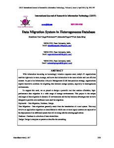
a) Key-value stores b) In-memory databases c) Graph analytics Figure 1: Effect of memory latency and bandwidth on the performance of large in-memory applications. looking at deploying DRAM and NVM based hybrid memory systems are justifiably concerned about the performance overheads due to the vast majority of the memory being several times slower than traditional DRAM. To illustrate the effect of NVM’s characteristics on an application’s performance, consider three different applications: (i) a Facebook like trace [21] running on the popular Memcached [10] and MemC3 [28] key value stores, (ii) standard TPC-C benchmark on the VoltDB [15] inmemory database, and (iii) a set of graph analytics frameworks [29, 41, 47, 52] running the Pagerank algorithm [23] on the Twitter dataset [34]. DRAM’s latency and bandwidth on this system are 150 ns and 40 GB/s, respectively. NVM technology is evolving and will likely exhibit a range of performance characteristics, depending on the details of the technology and the controller design. We therefore vary the parameters of our NVM emulator [39] to reflect this scenario by first varying the latency from 300ns to 600ns, while keeping the bandwidth the same as DRAM and then varying the bandwidth from 40 GB/s (same as DRAM) down to 5 GB/s (12.5% of DRAM), while keeping latency fixed at the worst case of 600ns. All applications are run in multi-threaded (or multi-process) mode, occupying eight cores. Figure 1 underlines that the performance impact across all application categories can be as much as 6× for NVM - that has 4× the latency and 18 × the bandwidth of DRAM. Depending on the actual implementation, these applications are sensitive to NVM’s higher latency or lower bandwidth or both. Streaming oriented applications (such as GraphMat and X-Stream) are particularly sensitive to NVM’s lower bandwidth, while the others (with lower bandwidth requirement) are more sensitive to NVM’s higher latency. To overcome the performance degradation in an “NVM only” system, future systems are likely to couple NVM with a smaller amount of DRAM, resulting in a truly heterogeneous memory architecture. A simple approach for dealing with the differing characteristics of DRAM and NVM in such systems is to treat DRAM as a cache for NVM and apply classic paging techniques to dynamically move data between them on demand. Unfortunately this solution leads to suboptimal performance for a number of reasons. First, it ignores the fact that objects with different access characteristics can be located on the same page, forcing co-located

objects to face the same treatment from the paging system. Second, paging comes with high overheads [17] that are unacceptable in general and particularly in the context of directly attached NVM where data does not need to be paged in to be accessed. In fact most of the applications considered in this paper explicitly forbid paging of their entire in-memory data (using mlock for instance), emphasizing the need for a more sophisticated solution than traditional paging. The first contribution of this paper is a quantitative study demonstrating that a large portion of this slowdown can be removed by judiciously placing some application data structures in the small amount of DRAM available in a hybrid memory system. The second contribution of this paper is showing that the performance impact of placing a data structure in a particular type of memory depends on the access pattern to it. This dependence is due to different memory access patterns – sequential, random and pointer chasing – having very different effective latencies on modern superscalar out-of-order processors. The frequency of accesses to application data structures by itself is not sufficient to determine the relative “hotness” of these data structures. The third contribution of this paper is the design and construction of a memory management infrastructure (called XMem) whose API allows programmers to easily map objects to data structures that they belong to at the time of object allocation. The implementation of X-Mem then places objects of different data structures in disjoint regions of memory, therefore preserving semantic information at the granularity of a single allocation. The fourth contribution of this paper is a profiling tool that automatically identifies the access pattern to a data structure and automates the task of mapping memory regions of that data structure to DRAM or NVM to optimize performance. The final result is optimal performance without programmers needing to reason about their data structures, processor behavior or memory technologies. Using a small amount of DRAM (only 6% of the total memory footprint for GraphMat, and 25% for VoltDB and MemC3) the performance of these applications is only 13% to 40% worse than their

DRAM based counterparts, but at much reduced cost, with 2× to 2.8× better performance/$. Intelligent data structure placement is the key to achieving this result, without which these applications can perform 1.5× to 5.9× worse on the same configuration, depending on actual data placement. Based on these results, we contend that a hybrid architecture offering both DRAM and NVM, where software has direct access to its different types of memories is indeed a realistic approach to building systems that can tackle the exponentially growing datasets at reasonable performance and compelling cost.

2.

X-Mem Design

X-Mem can improve application performance by automatically placing data-structures in appropriate memory types. However, in order to do that it must distinguish between objects belonging to different data structures. To solve this problem, X-Mem provides an expanded memory allocation interface that allows programmers to specify a tag during memory allocation. By using a unique tag for each data structure, programmers provide the necessary information for the X-Mem runtime to map each object to its data structure. Start Identify application data structures that scale with the memory footprint Tag the allocation of application data structures using the X-Mem API Placement objective

Memory configuration

Input

Input

for production run with X-Mem consists of the following two steps. (1) Tagging of the application data structures: Since the goal of tiering is to exploit the larger capacity of NVM, this step includes the manual effort of identifying the on-heap data structures that scale with the application’s memory footprint, and explicitly tagging the allocation of those data structures using the X-Mem allocator API (§2.1). (2) Automatic classification of the data structures: X-Mem’s automatic classification involves profiling an application to determine the benefit of placing an application data structure in DRAM vs. NVM, relative to the other application data structures. The output of this step, a tag-to-priority map that encodes these relative benefits, is then used by the X-Mem runtime to determine the optimal placement of application data structures. X-Mem’s automatic classification has some limitations due to its static nature and offline profiling. For one, it assumes homogeneous behavior within a data structure, which is a reasonable assumption for the applications and workloads considered in this paper (§5). A more generic solution would require efficient online tracking of the objects with the same tag. We plan to address this problem in future. Secondly, while tagging application data structures is a one-time effort, automatic classification is dependent on the workload. If the workload behavior changes dramatically, the current system requires another round of classification to adjust to the new behavior. Data centers often employ shadow infrastructure to test their code before deployment. One option is to periodically profile the workload in this shadow environment and re-classify the application data accordingly. 2.1

Profile run Enable the X-Mem profiler. Run the application with the X-Mem runtime. Derive the relative priority of data structures. Output

Tag->Priority

void* xmalloc(int tag, size_t size); void xfree(size); void xmem_priority(int tag, int prio); Figure 3: X-Mem API

Done

Input

Production run Disable the X-Mem profiler. Run the application with the X-Mem runtime.

Figure 2: An overview of tiering with X-Mem Figure 2 shows an overview of the process for tiering application data with X-Mem. The preparation of an application

Allocator API

Figure 3 shows the X-Mem API. The allocation routine (xmalloc) is the same as the standard malloc memory allocator API, except for the addition of a data classifier (or tag). In our current implementation, if an application wishes to change the tag of data after allocation, it has to explicitly allocate new data with the required tag and copy the old contents. xmem priority enables applications to explicitly assign priority values to the tags. Memory belonging to higher priority tags is preferred for placement in faster memory (DRAM). X-Mem applies automatic placement to break ties between data structures of the same priority. By default, all data structures have the same priority leaving X-Mem as the sole authority that determines placement.

X-Mem is designed to tier in-memory application data that is being scaled up over time. Such data is usually dynamically allocated on the heap, and therefore the X-Mem API is targeted at dynamic memory management. Statically allocated data structures and the program stack continue to be allocated in DRAM by the default runtime mechanisms. 2.2

Allocator Internals

Since the purpose of this work is placement in hybrid memory systems rather than optimizing memory allocators for NVM, X-Mem internally uses a standard memory allocator (jemalloc [2]) to manage memory. Unlike normal usage however, X-Mem instantiates a new jemalloc allocator for each tag that it sees. Each tag is therefore mapped to a unique allocator and all memory allocation and deallocation for objects with a particular tag are redirected to the memory allocator associated with the tag.

backing an existing virtual region from DRAM to NVM. We simply reissue an mbind call with the desired mapping for the region, leaving the operating system (Linux) to do the heavy lifting of actually migrating pages and updating page tables synchronously. We note that this process leaves the application-visible virtual addresses unchanged, allowing the application to continue running unmodified. Also, this design results in X-Mem being entirely restricted to user space, making it portable and easy to deploy as a library. Figure 4 shows an example of X-Mem’s data placement and migration policies. The application in this case allocates three data structures (tree, hash, and buffer) using the XMem API. Memory allocations for each of these data structures are managed by a separate jemalloc instance. The tags used by the application (T1 , T2 , and T3 ) are assigned internal priorities (§4) used to decide placement.

2.3

Mapping Regions to Memory Types

X-Mem maps regions to memory types based on its automatic placement algorithm that we describe later (§4). We expose NVM as a memory-only NUMA node separate from DRAM and use the mbind system call to restrict physical memory allocations for a region to a particular NUMA node – i.e., to DRAM or NVM.

DS3 (Buffer)

Application Data Structures

X-Mem assumes ownership of a large contiguous range in the application’s virtual address space (using mmap). This virtual address space is managed by a special “root” allocator. An allocator used to manage memory for a particular tag (data structure) grows or shrinks its memory pool in units of a region that is allocated (deallocated) from the root allocator. Each region has a fixed size that is a power of two for this paper we use regions that are 64 MB in size. At any given point, a region in use is assigned to exactly one jemalloc instance. All objects in a region therefore have the same tag. Unused regions belong to the root allocator. Some metadata (§4) is maintained for each memory region to guide placement decisions. A hash table of regions indexed by the start address of the region allows easy access to region metadata and the allocator owning the region. It is therefore easy to map an address to the start address of its containing region by masking the appropriate number of bits - the lower 26 bits for 64 MB regions. The start address of the region is used to index into the hash table and allows locating the appropriate allocator for xfree operations and region metadata. The metadata overheads are negligible compared to the 64 MB region size.

DS2 (Tree)

DS1 (Hash)

xmalloc(T1, )

Allocator 1

xmalloc(T2, )

xmalloc(T3, )

Allocator 2 X-Mem Allocator

Allocator 3

T2; T1; T3 Placement order

Application VA Migration

DRAM

NVM T1

T2

T3

Figure 4: X-Mem design

3.

Memory Access Time Model

X-Mem supports automatic assignment of virtual memory regions to physical memory types to optimize performance. Optimum placement is based on a model of memory access time in superscalar processors that we now describe. For working sets that do not fit in the last level cache, every accessed cacheline is equally likely to result in a miss under the assumption of lack of temporal locality due to uniformly distributed accesses over the working set. For brevity in notation, we consider the case of N data structures in a program. Let Si be the stall time for each access to data structure i and let Ci be the count of the number of accesses made to the data structure from a single thread. The average time for a memory access:

N

At run time, as new memory regions are added to the program, the newly added regions can displace memory regions from DRAM. This displacement causes X-Mem to trigger migration to change the type of physical memory

∑ Ci ∗ Si A=

i=1 N

∑ Ci i=1

(1)

The stall latency of each access in a modern superscalar processor is not the same as the time to access memory. The processor can hide the latency to access memory by locating multiple memory requests in the instruction stream and then using out-of-order execution to issue them in parallel to memory via non-blocking caches [39]. In addition, microprocessors incorporate prefetchers that locate striding accesses in the stream of addresses originating from execution and prefetch ahead. As a result the effective latency to access memory can be much smaller than the actual physical latency for certain access patterns.

Latency (in ns)

The stall for each access to the data structure clearly depends on the latency to memory, which in turn is determined by the type of memory that the data structure is placed in. However that piece of information alone is insufficient.

Table 2 shows a classification of the memory accesses along two axes – sequential vs. non-sequential and independent vs. dependent. One of these access patterns (sequential and dependent) rarely appears in the real-world applications, and we therefore ignore that pattern. We illustrate the effects of the processor’s latency-hiding features using a set of microbenchmarks that consider the other three access patterns: • Random: The instruction stream consists of independent

random accesses. The processor can use its execution window to detect and issue multiple requests simultaneously. • Pointer chasing: The processor issues random accesses

but the address for each access depends on the loaded value of a previous one, forcing the processor to stall until the previous load is complete. • Streaming: The instruction stream consists of a striding

access pattern that can be detected by the prefetcher to issue the requests in advance. In Figure 5 we vary the latency and bandwidth characteristics of memory in our NVM performance emulator (§5.1). Pointer chasing experiences the maximum amount of stall latency, equal to the actual physical latency to memory. In the case of random access, out-of-order execution is effective at hiding some of the latency to memory. In the case of streaming access, the prefetcher is even more effective at hiding latency to memory. The order of magnitude difference in the performance of these access patterns validates our observation that the frequency of accesses alone is not sufficient to determine the “hotness” of a data structure, and illustrates the need for the more sophisticated classification of memory accesses proposed in this paper.

100

10 1

DRAM

300-10

Pointer

Random

450-10

600-10

Streaming

Figure 5: Memory read latency for various access patterns. The microbenchmarks give us an effective way to measure the average stall latency for different types of accesses and data structures. We use L(p, m) to indicate the stall latency for accesses of pattern p to memory of type m.

4. Dependent Independent Sequential NA Streaming Non-sequential Pointer chasing Random Table 2: Overview of memory access patterns

1000

Profile Guided Placement

Optimizing placement in X-Mem works as follows. First, we use a profiler to determine the relative frequency of different types of access to each data structure (tag). Second, during production runs the profiling data is used to maintain a list of memory regions sorted by preference for their placement in faster memory (DRAM). As many regions as possible from the head of the list are mapped to DRAM leaving the rest in slower NVM. We first describe our profiler and then describe how the profile data is used by X-Mem at runtime. 4.1

Profiler

Figure 6 shows the process of profiling and automatic classification with X-Mem. We use a profiling tool that operates in conjunction with the X-Mem memory allocator described in §2. For each data structure tag, the tool classifies accesses to its regions as one of random, pointer chasing and streaming, and counts the number of accesses of each type. Note that we modify the application only once to use the X-Mem API for memory allocation, and use the same binary for profiling and the actual production run. The profiler uses PIN [37] to intercept memory accesses and record (for each access) the address that was accessed. This information is stored in a buffer and processed periodically (every 1024 memory operations, by default) using the post-processing algorithm shown in Figure 7. For each window of memory operations, we first sort the accesses in the buffer, effectively grouping accesses to the same region together. We iterate through the buffer searching for access pairs where the value at the location of the first access equals the address of the location of the second access. We interpret this pattern as pointer chasing to the second location and attribute the stall latency to the second access. To comprehend the more complex addressing modes (base register plus an offset), we use PIN’s facility to record the contents of the base register used for address generation rather than the entire effective address. We also maintain a sliding window (of

Start

Run the workload with the X-Mem profiler enabled Capture a window of memory operations to the address range managed by X-Mem No

Process the memory trace. Update (per region) memory access pattern statistics.

Input: A buffer of addresses Sort the buffer by address sliding_window = () for each access i in sorted buffer: if exists access j in sorted buffer s.t. j.address == *i.address and Cacheline(j.address) != Cacheline(i.address) region[j.address].pointer_chasing++

End of run?

if Cacheline(i.address) != Cacheline(sliding_window.end().address) Advance sliding_window to include i if sliding_window is a strided pattern Region[i.address].streaming++ Region[i.address].accesses++ if i is a read Region[i.address].reads++ else Region[i.address].writes++

Yes

Access statistics Input

Convert per region statistics to per data structure statistics

Placement objective Input

Figure 7: Classifying Access Type

Run X-Mem placement algorithm. Compute per data structure benefit of placement in DRAM. Output

Tag->Priority

Done Figure 6: An overview of the profiling step with X-Mem size 8 by default) over elements of the sorted buffer to detect streaming accesses where consecutive elements of the window differ by the same amount. We also count the total number of accesses to a memory region. Subtracting the number of streaming and pointer chasing accesses from this total number gives us the number of random accesses. In the post-processing algorithm we eliminate accesses to the same cacheline assuming that the set of accesses in the buffer would fit in cache and repeated accesses to the same cacheline do not go to memory. The cost of post-processing the buffer grows slowly with the size n of the buffer as O(nlog(n)) and therefore we are able to use a large buffer (of size 8KB) to amortize the cost of switching the context from running the application to running the analysis routine. As described in §2 we maintain metadata for each memory region and are able to access the metadata starting from an address via a hash index. This metadata includes the counters we use in Figure 7. After the program terminates, we roll up the counters from all memory regions for a particular data structure into a permemory region average that is attached to the parent data

structure (tag). This average consists of three counters – one each for pointer chasing, random and streaming accesses. Since data structures can have different kinds of accesses (such as traversing a linked list and then accessing fields of a particular node), we do not attempt any further classification of the data structure. We use Fi (p) to denote the fraction of accesses of pattern p to data structure i as read from these counters. 4.2

Runtime

The runtime estimates Equation 1 using the profiling information. Let T (r) be the type of memory in which memory region r is placed and let D(r) be the parent data structure of r. We estimate the memory access time for a given configuration as follows:

Aˆ =

∑

∑

FD(r) (p)L(p, T (r))

(2)

r∈Regions p∈Patterns

We use the profiling run estimate of the average number of accesses of a particular pattern to a memory region, and then multiply it by the appropriate latency of that access pattern. The placement algorithm aims to minimize the quantity Aˆ by choosing the right assignment of memory regions to memory types, while respecting the capacity constraints of each type of memory. Since this paper deals with only two different types of memory (standard DRAM and slower NVM), we cast this problem as follows.

We start by assuming that all regions are in NVM. Given a fixed amount of faster DRAM, moving some memory regions to DRAM would reduce the average access time. Hence the problem is to choose a set of memory regions moving which maximizes the gain. For any memory region r the benefit of moving to DRAM is:

B(r) =

∑

FD(r) (p)[L(p, NV M) − L(p, DRAM)] (3)

p∈Patterns

The estimated average access time in a hybrid memory system can therefore be rewritten as follows:

Aˆ =

∑

∑

r∈Regions p∈Patterns

FD(r) (p)L(p, NV M) −

∑

B(r)

r∈DRAM

(4) To minimize Aˆ we need to maximize the second term. We have a fixed number of slots in DRAM into which we can place memory regions and a fixed real quantity B(r) that quantifies the benefit of putting memory region r in DRAM. We use a greedy algorithm to maximize the total benefit by first sorting the regions into a list ordered by decreasing benefit, and then placing regions starting from the head of the list into DRAM until no more space is left in DRAM. This algorithm is optimal because any placement that does not include one of the chosen regions can be further improved by replacing a region not in our chosen set with the missing region. We note that the benefit B(r) is the same for all memory regions of a particular data structure. Therefore we compute this quantity as a property of the data structure itself and use it for each memory region of the data structure. 4.3

Loaded Latency

Our model ignores queuing delays caused by traffic from other cores. In Equation 3, we use the difference in latencies of access to NVM and DRAM. Requests to all types of memory (for all access patterns) follow the same path from the core to the memory controller before being dispatched to the appropriate memory channel. The queuing delays are therefore the same for both types of memory and cancel out.

5.

Evaluation

We evaluate X-Mem using a set of representative applications: a high-performance graph analytics framework (GraphMat), an in-memory database (VoltDB), and a keyvalue store (MemC3). All three applications work on data

sets that can be scaled up and therefore have potential to benefit from the larger capacity and lower cost of NVM in a hybrid memory system. The evaluation has two objectives. The first is to show that the performance of all three applications depends significantly on the placement choice for each data structure in them. Second, we aim to show that our placement technique (§4) correctly identifies access patterns to each data structure and enables optimal data placement with X-Mem. To demonstrate the results - in all cases - we provide two baselines for comparison. The first is NVM-only – in which an application’s memory is allocated entirely from NVM. NVM-only depicts the worst case performance of unmodified applications in a hybrid memory system. The second is DRAM-only, which represents the best-case performance of an application when all accessed data is allocated in fast DRAM. We perform all experiments on a hybrid memory emulator (§5.1) that runs at full speed. For the network-based applications (Memcached and VoltDB), we use a dedicated machine to run clients that drive the application under test. The client machine is connected directly to the server (with no intermediate switch) via multiple 10 GigE NICs, therefore ensuring that neither the network nor the clients are limiting the performance and we can focus entirely on the interaction with main memory. Although NVM technologies have been announced by some manufacturers [1], the industry is still actively developing the first generation of NVM as well as the controllers to which they will be attached. As a result, till the technology matures, one can expect a spectrum of performance characteristics from NVM, rather than a single point. For proper sensitivity analysis, we therefore use the hybrid memory emulator to study a range of NVM latency and bandwidth characteristics to obtain broad applicability for our results. 5.1

Hybrid Memory Emulator

The hybrid memory emulation platform (HMEP) [39] was built by Intel to support the exploration of software stacks for hybrid memory systems. HMEP enables the study of hybrid memory with real-world applications by implementing – (i) separate physical memory ranges for DRAM and emulated NVM (using a custom BIOS), and (ii) fine-grained emulation of configurable latency and bandwidth for NVM (using custom CPU microcode). HMEP is restricted to Intel proprietary Xeon E5-4620 platforms, with each of its two processors containing eight 2.6 GHz cores. Hyperthreading is disabled. Each CPU supports four DDR3 channels and memory is interleaved across the CPUs. The measured DRAM latency and bandwidth on the system are 150ns and 37GB/s, respectively. HMEP has been used before in other research [20, 26, 27, 43, 44, 56], and described in detail elsewhere [39]. A sufficient number of

5.2

Modifications to use the X-Mem API

Modifying applications to use the X-Mem API involves very few (10 to 50) lines of code in any of the applications. For each application, we first identify data structures that grow with the size of the application data and occupy significant portions of the application’s memory footprint. Only such large data structures are allocated using the X-Mem API; other data continues to be allocated in DRAM using the default system allocator. Each data structure is given a unique tag. We are exploring options to automate the process of attaching a unique tag to each data structure, perhaps as compiler extensions.

6.

GraphMat

Exploding data sizes leads to a need for large-scale graphstructured computation in various application domains [38]. Large graph processing, however, lacks access locality and therefore many graph analytics frameworks require that the entire data fit in memory [29, 38, 52]. We study a high performance in-memory graph analytics framework called GraphMat [52] that implements a vertexcentric scatter-gather programming model. The performance of graph analytics frameworks (like GraphMat) depends

30

Read

Write

25 20 15 10

5 0

Time

100

% of physical memory latency

We present results for six HMEP configurations that represent the performance spectrum for NVM (Table 1). In these configurations, NVM’s latency ranges from 2× to 4× of DRAM latency (300ns, 450ns, and 600ns), and NVM’s bandwidth varies from 41 × to 18 × of DRAM bandwidth (10GB/s to 5GB/s). In addition, we also evaluate different ratios of NVM to DRAM sizes in the system. We use 1/T to refer to a setup where the DRAM size is 1/T of the total available memory in the system. In all the tests, we give a fixed amount of total memory (equal to the sum of DRAM and NVM) to the application. Corresponding to these setups, we also consider the cost of the total memory. For generality, NVM cost is derived from prior research that expects NVM (PCM) based SSDs to be 4× more expensive than enterprise MLC NAND flash SSDs [33]. Based on the prevalent prices of DDR-based DRAM [19] and a conservative estimate that directly addressable NVM devices presumed in this work will be more expensive than NVM-based SSDs (at least initially), we assume that DRAM is 5× more expensive than NVM on cost-per-bit basis. Since memory costs significantly higher than other server components in large memory systems of interest to this paper, we use the above cost estimate as the proxy for total server cost.

both on the topology of the graph and the specific algorithm [39, 48, 52].

Bandwidth (in GB/s)

HMEPs are available to researchers such as us to both enable the exploration of NVM configurations at full speed (avoiding the overheads of simulation) as well as to enable easy reproduction of results of others using HMEP.

80 60 40 20 0

Time

a) Memory bandwidth b) Effective memory latency Figure 8: Memory usage in GraphMat (Pagerank algorithm). Test details: Since the topic of this paper is not graph processing, we present results only from execution of the Pagerank algorithm [23] on a large graph representing the Twitter follower network [34]. The graph has 61.5 million vertices and 1.4 billion edges. The Pagerank algorithm on this graph ranks users by connectivity to influential followers to identify the most influential individuals in the sample of the Twitter network captured in the dataset. The memory footprint of the workload is approximately 32GB. Figure 8 shows the bandwidth requirements and the effective latency of GraphMat when running the test. Effective latency, shown as percentage of the actual physical memory latency, approximates the average memory read latency in an application by measuring the core stalls due to pending reads per last level cache miss. GraphMat can achieve very high bandwidth usage (of up to 25GB/s read and 15GB/s write bandwidth) but its effective latency is low (mostly under 20%) due to GraphMat’s ability to exploit CPU’s MLP. GraphMat’s performance is therefore highly sensitive to lower bandwidth, but only to some extent to higher latency. This explains the degradation in the NVM-only performance of GraphMat with the decrease in bandwidth rather than increased latency (Figure 9a). 6.1

Data Structures and Placement

GraphMat takes vertex programs and maps them to highly optimized, scalable sparse matrix operations in the backend. GraphMat implements graph algorithms as iterative generalized sparse matrix-sparse vector multiplication (or SPMV) that updates some data associated with the vertices (e.g., Pagerank). Graphmat has three main data structures: a sparse vector, a dense vector of vertex data and finally the adjacency matrix of the graph in compressed sparse row format. The sparse vector of vertex data is built on every iteration and consists of the data from active vertices in the computation. By reading from and writing to the sparse vector rather than the full dense vector of vertices, Graphmat achieves better cache efficiency. We modify GraphMat to use xmalloc for these three data structures.

Data structure Sparse Vectors Vertex Data Adjacency Matrix

%Size 3.5 2.4 94.1

%Accesses 92.64 1.53 5.83

%pointer 0.0 0.0 0.0

Access pattern %seq %random 0.34 99.64 13.98 86.02 0.0 100.0

Benefit per region %writes 32.75 56.02 0.0

3948.06 67.05 9.30

Table 3: Memory tiering in GraphMat with the X-Mem API. 1400 1000

600

1000

Normalized perf/$

Time (in seconds)

100 10

200 300-10 450-10 600-10 300-5 450-5 600-5 NVM Latency(ns)-Bandwidth(GB/s) NVM-only

1/32

1/16

a) Tiering performance

1/2

3 2

1 0

300-10 450-10 600-10 300-5 450-5 NVM Latency(ns)-Bandwidth(GB/s)

SPMV

Other

DRAM-only

Total

NVM-only

1/32

1/16

600-5

1/2

b) Breakdown of time taken (at 600-5) c) Tiering performance/$ Figure 9: Evaluation of memory tiering in GraphMat.

Table 3 illustrates the inner workings of X-Mem’s automatic placement algorithm. We provide the sizes of the three GraphMat data structures (relative to the total memory footprint) in the second column, and the relative access frequencies of those data structures in the third column. The most frequently accessed data structure is the sparse vector, followed by vertex data and finally by the adjacency matrix. The next group of columns breaks down the accesses to each data structure as pointer chasing, sequential scans and random accesses. For the sake of completion, we also show the percentage of accesses to the data structures that are writes. The access to the sparse vector and adjacency matrix is largely random. The access to the vertex data is somewhat sequential - depending on the active vertices accessed at every pass to build and tear down the sparse vector. The product of the fraction of accesses and the fraction of a particular type gives us the Fi (t) quantity for that particular data structure (Equation 3). In the last column of the table, we show the benefit computed by the placement algorithm for the 450-10 configuration of NVM. The placement algorithm prioritized the sparse vector for placement in DRAM followed by the vertex data and finally the adjacency matrix. Figure 9a shows the performance of Graphmat with varying memory configurations and X-Mem’s adaptive placement enabled. GraphMat’s performance for NVM-only is worse than that for DRAM-only by 2.6× to 5.9×, with the drop in performance particularly steep at lower peak NVM bandwidth. Most of the performance gap can be attributed to sparse vectors, which account for only 3.5% of GraphMat’s footprint (of 32GB). Figure 9b depicts this overwhelming contribution of SPMV operations, which use sparse vectors, to the overall run time of GraphMat. Performance improves dramatically with 1/32 tiering – only 1.17× to 1.55× worse than DRAM-only – because X-Mem is able to place sparse vectors in available DRAM. With 1/16 tiering, X-Mem can allocate vertex data (less than 2.5% of the total footprint) in DRAM and that improves tiered GraphMat’s performance

to within 1.13× to 1.4× of DRAM-only. Beyond 1/16, performance is limited by uniform (bandwidth-bound) accesses to the large adjacency matrix. Hence, 1/2’s performance is 1.09× to 1.29× of DRAM-only, a minor improvement over 1/16 but at much higher cost. From the cost viewpoint, 1/32’s performance/$ is 2.9× to 3.8× that of DRAM-only and 2× to 3.4× compared to NVM-only. 1/16 is only slightly behind 1/32 – 1.83× to 2.5× compared to DRAM-only. Interestingly, 1/2’s performance/$ is worse than that of DRAM-only and NVM-only across all HMEP configurations.

7.

VoltDB 5

Bandwidth (in GB/s)

DRAM-only

4

Read

Write

4

3 2 1

0

Time

% of physical memory latency

Time (in seconds)

1800

100

80 60 40

20 0

Time

a) Memory bandwidth b) Effective memory latency Figure 10: Memory usage in VoltDB (TPC-C workload). In-memory databases exploit architectural and application trends to avoid many overheads commonly associated with disk-based OLTP databases [12, 13, 15, 51]. VoltDB, one such in-memory database, is an ACID-compliant, distributed main memory relational database that implements the sharednothing architecture of H-Store [51]. Test details: For the results in this paper, we run the industry standard TPC-C benchmark, which models the operations of a wholesale product supplier [14]. We set the number of warehouses to 512 and the number of sites in VoltDB to 8, resulting in a 40GB memory footprint. The TPC-C throughput is reported in total transactions per second. Figure 11 shows that VoltDB’s performance is sensitive only to memory latency, which can be explained by the high

Data structure

%Size

IDX ORDER LINE TREE IDX S PK HASH CUSTOMER IDX O U HASH STOCK ORDER LINE IDX OL PK HASH HISTORY IDX CUSTOMER NAME TREE CUSTOMER NAME

%Accesses

4.73 1.16 0.66 0.52 20.36 11.61 5.73 0.94 16.43 35.90

%pointer 48.97 49.55 0.06 3.01 0.0 0.01 8.68 2.03 32.76 0.0

43.32 2.7 3.28 0.17 16.57 5.98 1.69 0.25 1.65 0.59

Access pattern %seq %random 0.12 50.91 0.0 50.45 0.0 99.94 0.0 96.99 0.0 100.0 0.33 99.66 0.95 90.37 0.0 97.97 0.0 67.24 0.0 100.0

Benefit per region %writes 27.07 0.0 7.19 69.33 5.55 28.59 55.89 56.51 0.0 0.0

190.17 56.14 27.92 5.99 5.31 5.13 4.81 4.27 1.93 0.11

25

20 15

10 300-10 450-10 600-10 300-5 450-5 600-5 NVM Latency(ns)-Bandwidth(GB/s) DRAM-only

NVM-only

1:16

1/4

a) Tiering performance

1/2

100 80 60 40 20 0

Normalized perf/$

% of transactions

TPS (in thousands)

Table 4: Memory tiering in VoltDB with the X-Mem API. 30

25

50

75 100 125 150 175 200 Transaction latency (in ms)

DRAM-only

1/16

Data Structures and Placement

VoltDB scales by horizontally partitioning the tables across multiple single-threaded engines (called sites) and replicating the partitions. We modify VoltDB to allocate indices and tables using xmalloc. Overall, TPC-C in VoltDB contains 28 such data structures, of which the top 10 data structures (size-wise) account for approximately 99% of the total memory footprint. Table 4 illustrates the application of X-Mem’s placement algorithm to these top 10 data structures. Intermediate results and other data structures are allocated in DRAM using the default system allocator. Figure 11a shows that NVM-only’s performance is 26% to 51% worse than that of DRAM-only, a better situation than Graphmat because TPC-C is comparatively less memoryintensive. 1/16 performs better than NVM-only by 24% to 48%, by enabling X-Mem to place temporary data and three frequently accessed data structures – tree-based secondary index for the ORDER LINE table, hash-based primary index for the STOCK table, and the small CUSTOMER table – in DRAM. 1/8 (not shown here to avoid clutter) and 1/4 do not perform much better than 1/16. At 1/2 X-Mem is able to place all the data structures of VoltDB in DRAM, barring the very large, but infrequently used, CUSOMTER NAME

3 2

1 0

300-10 450-10 600-10 300-5 450-5 NVM Latency(ns)-Bandwidth(GB/s)

1/2

b) Transaction latency distribution at 600-5 Figure 11: Evaluation of memory tiering in VoltDB.

effective latency – of over 50% at times (Figure 10b) – caused by random accesses in VoltDB (particularly to the indices). VoltDB consumes an average read bandwidth of 2.3GB/s and write bandwidth of only 1.3GB/s for the TPC-C workload (Figure 10a), and is therefore insensitive to lower bandwidth. 7.1

NVM-only

4

DRAM-only

NVM-only

1:16

1/4

600-5

1/2

c) Tiering performance/$

table and some portions of the tree-based primary index for the same table. As a result, 1/2’s performance is 35% to 82% better than NVM-only and only up to 9% worse than DRAM-only. Figure 11b shows the latency distribution of TPC-C transactions, since it is an important metric for OLTP workloads. Average transaction latency increases as we move to configurations with more of the data in NVM. However the increase is moderated by the placement algorithm that results in transaction latencies close to that for DRAM even for a 1/16 configuration. 1/16’s performance/$ is better than DRAM-only by 2.5× to 3.7×, and best across most HMEP configurations. The only exception is 300-10, where NVM-only provides better performance/$ than 1/16. More importantly, all of the tiering options offer better performance/$ than the DRAM-only option. 1/2’s performance/$ is, for instance, 1.5× to 1.7× better than DRAM-only, while providing within 9% of DRAMonly’s performance.

8.

MemC3

Key-value stores are becoming increasingly important as caches in large data centers [21]. We study a variation of Memcached [10] called MemC3 [28] – a recent advance over the open source Memcached that improves both memory efficiency and throughput over the stock implementation. MemC3 implements a variant of cuckoo hashing to avoid expensive random dependent accesses that are common in Memcached. In addition, MemC3 replaces Memcached’s

Bandwidth (in GB/s)

15

Read

Write

12 9 6 3 0

Time

% of physical memory latency

exclusive, global locking with an optimistic concurrency control scheme. 100 80 60 40 20 0

Time

a) Memory bandwidth b) Effective memory latency Figure 12: Memory usage in MemC3 (Facebook-like workload). Test details: Key-value stores (such as Memcached and MemC3) are used in widely different scenarios. Unlike with OLTP databases, there is a lack of standard benchmarks for key-value stores. We base our test workload on data recently published by Facebook [21, 42], specifically on the ETC trace. To test MemC3 in a deterministic manner, we modified memaslap [9] to implement separate load and execution phases (similar to YCSB [16] but without requiring the traces to be saved to a file). During the load phase, the MemC3 server is populated with a dataset of approximately 64GB. The key size is fixed at 16 bytes and the size of the values ranges from 16B to 8K, roughly following the distribution of values in the ETC trace in Facebook’s published data [21]. More than 90% of the values are 512 bytes or less in size. However, values greater than 512 bytes occupy almost 50% of the cache space. The total memory footprint of the workload is approximately 100GB. During the execution phase, the client generates 50 million random queries based again on the value distribution in the ETC request trace. The workload is read heavy (95% GET and 5% SET) and currently does not contain any DELETE requests. We report the total time to complete the test. Figures 12 shows the performance characterization of MemC3 with the client requesting values of one size at a time (from 16B to 8K). Figure 12a shows that MemC3’s read bandwidth ranges from 1.8 GB/s to 14 GB/s and write bandwidth ranges from 1 GB/s to 6.5 GB/s, depending on the size of the value. Effective latency decreases (from 48% to 4%) at larger values, due to improved sequential performance (Figure 12b). MemC3’s sensitivity to higher latency rather than lower bandwidth, as depicted by NVM-only’s performance in Figure 13a, is explained by the large skew towards the smaller values in our workload. Figure 13b further illustrates this fact by breaking down NVM-only’s overheads at various value sizes.

8.1

Data Structures and Placement

MemC3 allocates memory for the cuckoo hash table at startup and employs a dynamic slab allocator to allocate values, with the slab type determined by the size of allocation from the slab. The hash table and the slabs are all allocated using xmalloc, resulting in a total of nine data structures in X-Mem (Table 5) since each slab type is treated as a separate data structure. Table 5 shows the priorities of these data structures as determined by the X-Mem placement algorithm. Note that the priorities determined by X-Mem for the various slab types fully follow the value-wise breakdown of NVM-only’s overhead in Figure 13b, demonstrating the accuracy of XMem placement model. Table 5 also shows why the frequency of accesses to a data structure alone is insufficient for determining the benefit of placing it in faster memory. The cuckoo hash and 256B, for instance, are relatively close both in terms of their access frequencies and memory footprint, but contrast in terms of benefit per memory region due to their different access patterns. Figure 13a shows that, depending on the HMEP configuration, NVM-only’s performance is 1.15× to 1.45× worse than that of DRAM-only. With 1/8 tiering, where only 12.5% of the application data is in DRAM, performance improves by 8% to 17% over NVM-only because X-Mem allocates MemC3’s cuckoo hash DRAM. 1/4 fares even better and improves the performance to within 6% to 13% of DRAMonly, mainly because X-Mem is now able to place a large number of small values in DRAM and reduce the number of random accesses to NVM. Increasing the amount of available DRAM beyond 1/4 results in incremental improvements, and eventually at 1/2, performance overhead over DRAM-only is within 5%. However, this improvement comes at much higher cost as depicted in Figure 13c. NVM-only provides best performance/$ across all HMEP configurations – 3.5× to 4.5× compared to DRAM-only, mainly because the NVM-only overhead is relatively low. Finally, all tiering options provide significantly better performance/$ (1.6× to 3.1×) than DRAM-only, resulting in a range of interesting performance/cost tradeoffs.

9.

Practical Deployment

X-Mem is intended for deployment with soon to be introduced NVM based systems [30]. Therefore, design choices in X-Mem were made with the following practical considerations.

Data structure Cuckoo hash 16B, 32B, 64B 256B 128B 4096B 512B 1024B 2048B 8192B

%Size

%Requests

12.35 8.64 18.52 16.05 6.17 4.32 4.94 10.49 18.52

%Accesses

NA 55.0 16.0 24.0 2.0 1.0 1.0 0.7 0.3

17.65 23.51 16.29 8.48 10.47 2.01 3.41 7.67 10.5

%pointer 21.15 0.0 0.0 0.0 0.0 0.0 0.0 0.0 0.0

Access pattern %seq %random 0.0 78.85 0.0 100.0 0.0 100.0 0.0 100.0 91.95 8.05 21.02 78.98 72.21 26.79 86.5 13.5 94.32 5.68

Benefit per region %writes 3.44 18.63 13.37 15.41 4.98 10.98 6.78 5.49 4.49

83.76 70.53 22.77 13.7 13.3 10.35 9.01 7.7 5.11

Table 5: Memory tiering in MemC3 with the X-Mem API. Time (in seconds)

Time (in seconds)

30 25

5

0

20 300-10 450-10 600-10 300-5 450-5 600-5 NVM Latency(ns)-Bandwidth(GB/s)

DRAM-only

NVM-only

1/8

1/4

a) Tiering performance 9.1

Normalized perf/$

10

35

1/2

16B 32B 64B 128B 256B 512B 1K Value size DRAM-only

NVM-only

2K

1/8

4K

8K

1/4

5 4 3 2

1 0 300-10 450-10 600-10 300-5 450-5 NVM Latency(ns)-Bandwidth(GB/s) DRAM-only

NVM-only

1/8

1/4

600-5

1/2

b) Tiering performance breakdown c) Tiering performance/$ Figure 13: Evaluation of memory tiering in MemC3.

Human Overhead

X-Mem offers a powerful yet simple API for applications to express important semantic information about their data. While replacing malloc and free with xmalloc and xfree is straightforward, assigning unique tags to individual data structures might require more effort depending on the implementation. In our case, modifying VoltDB required the most effort, but still involved changes to under 50 lines of code. The effort is considerably lower for object oriented programs where a class-specific allocator can be defined for calling xmalloc, rather than scattering those calls across the code. While the process is not onerous, it still requires manual effort and a good understanding of application source code. We plan to explore techniques to automatically tag the dynamic allocation of application data structures, at the least in the context of managed languages and runtimes [24, 32, 50]. Beyond tagging application data, no further effort or reasoning is necessary on the part of the programmer since the automatic placement algorithm does a job at least as good as a human programmer in placing data structures. To verify this claim, we repeated the experiments with other possible orderings of data structures for placement in DRAM. In case of VoltDB and MemC3, because of the large number of data structures, we selected a subset of the possible permutations that we deemed most optimal; for instance, based on the access frequencies alone and/or our understanding of the applications. For Graphmat we evaluated all possible permutations. In no case were we able to outperform our automatic placement algorithm. For example, with GraphMat, we were able to run all possible permutations for placement, with one instance (1/16 tiering at 600-5), showing that the placement

model’s suggestion was 1.0× to 5.8× better than the alternatives. 9.2

Profiling Overhead

Memory tracing (with Pin) during the profiling step can significantly slow down the application (up to 40× in our tests), and is therefore suited only for offline use and not for production. One option that we considered is to employ sampling based profiling [55]. The idea was shelved due to concerns that sampling profilers may fail to capture relationships between closely spaced memory accesses such as pointer chasing and strided scans. We are currently exploring extensions to the x86 ISA that would enable necessary profiling but without the expensive process of tracing each memory access. Such hardware extensions would enable real-time measurement and placement in X-Mem. The profiler however remains the solution for initial deployment. We also found that it is useful to downsize the workload while preserving the relation between its various data structures, in order to reduce the time spent in profiling. For instance, in the case of MemC3, we resize the number of values and the number of requests in the workload proportionately to the original distribution. 9.3

Device Wear

Device wear is a significant concern for the initial generation of NVM devices. With X-Mem based tiering, the applications and OS continue to use DRAM from the default system allocator for small temporary data and program stack, while X-Mem prioritizes the use of the remaining DRAM

Region Size Time (in ms)

64M-S 1015

512M-S 972

1G-S 924

1G-L 378

Table 6: Time taken to migrate one gigabyte of application data from DRAM to NVM (at 600-5). S and L denote the use of 4K pages and 1G pages respectively.

% of writes to NVM

for frequently used important application data. In that regard, X-Mem acts as a natural guard against wear by moving the most frequently accessed (and written) data structures to DRAM. Figure 14 shows that, depending on the mix of DRAM and NVM, X-Mem reduces writes to NVM by 48% to 98% (over NVM-only) in the applications evaluated in this paper. 100 80 60 40 20 0

MemC3 NVM-only

1/32

VoltDB 1/16

1/8

GraphMat 1/4

1/2

Figure 14: Writes to NVM as a percentage of total writes This work prioritizes performance over reducing wear, but it is possible to configure X-Mem to instead prioritize writeintensive data structures for placement in DRAM. The actual device wear, like performance, would depend on a number of factors – the granularity of wear-leveling, presence of power fail-safe DRAM buffers in NVM device, etc. As part of our future research, we plan to measure the effect of tiering on device wear and the total cost of ownership. 9.4

Migration Overhead

X-Mem performs “synchronous” migration by waiting for the mbind call to return when a memory region is migrated from DRAM to NVM. The overhead of this migration is negligible in our experiments due to the relatively small amount of time spent in allocations compared to the overall run time of the application. Table 6 shows the raw overhead of migration for region sizes ranging from 64M to 1G. 1G regions can amortize the cost of migration by 5% to 8% over smaller regions. The real benefit of using 1G regions however is that it allows the use of large (one gigabyte) hardware pages on most 64-bit servers; thereby further reducing the migration overhead by 60% compared to the baseline with 4K pages (1G-S). While we understand the benefits of using 1G regions with large pages in applications with large memory footprint [27], the current implementation of X-Mem uses 64 MB regions (by default) to reduce internal fragmentation. Also, X-Mem uses 4K hardware pages due to limitations in the Linux kernel w.r.t. enforcement of memory policies on large pages. We plan to address this situation in the future.

10.

Related Work

Qureshi et al. [46] propose a 2-level memory (2LM) architecture where DRAM is used as transparent hardware managed cache to NVM. We focus only on software managed hybrid memory systems and techniques to achieve optimal performance with them. Lim et al. [35] study the use of slow memory in the context of shared, network-based (disaggregated) memory and conclude that a fast paging-based approach performs better than direct access to slow memory. While their choice of target applications is key to their findings, their work also relies on a simple processor model that does not account for CPU’s MLP. In our experiments, we found that paging to NVM is several times slower than even the corresponding NVM-only solutions. Others have made similar observations regarding the performance of paging in Linux [17]. AutoNUMA monitors memory usage of applications in NUMA platforms and co-locates their memory with compute (via scheduling and migration) for optimal performance [3]. Data co-location in NUMA platforms, however, is very different from data placement in hybrid memory systems, where NVM is slow to access from all computations. AutoNUMA does not solve the problem of matching application data with physical memory. NVML is an open source implementation of allocators and abstractions optimized for NVM, both for persistent and volatile usage [11]. Like X-Mem, one of the goals of NVML is to exploit NVM’s capacity and cost attributes. But, XMem’s objectives go beyond that of NVML. For one, XMem alleviates applications from the responsibility of understanding the system’s topology, properties of memories, data migration at runtime, etc. Second, application-driven memory tiering with X-Mem has much broader scope and the X-Mem runtime can be extended to support any future hybrid system irrespective of the memory technology [6, 7]. SSDAlloc is a hybrid memory manager with a custom API that enables applications to use flash-based SSDs as an extension of DRAM [22]. In comparison, X-Mem is designed for hybrid memory systems where all memories are directly accessible to software and there are no overheads related to block-based accesses. Data classification is a well-studied problem in the context of traditional block-based storage [5, 40, 49]. Mesnier et al. [40] propose the classification of I/O data at block granularity to enable differentiated storage services (DSS) for traditional file and storage systems. A DSS classifier is internally translated to a relative priority based on a pre-defined policy that was assigned to the file by software. Data classification in X-Mem is finer grained and preserves semantic information at the granularity of a single allocation. As a result, X-Mem enables optimal data placement between

memories whose performance is not necessarily orders of magnitude apart. An alternative to dynamic tracing of memory accesses is static analysis to determine the access pattern to various data structures. However, since we target unmanaged languages, static analysis would require some form of “pointsto-analysis” [50] to map memory accesses through pointers to the actual types that they refer to. Since points-to-analysis is necessarily conservative it leads to situations where an access maps to more than one type or data structure, therefore resulting in inaccurate attribution of accesses. In addition static analysis does not give dynamic access counts; for example, the number of accesses within loops whose iteration count is input dependent. Dynamic access counts are critical to the model we use for placement decisions. Linux allows applications to provide hints about their use of virtual memory using the madvise system call [8]. The OS is free to act on or ignore those hints. Jantz et al. [31] propose a page coloring framework for applications to dynamically attach an intent to a group of pages. The applications and OS collaborate in a feedback loop to execute on (or fine tune) the intents. Others have demonstrated the benefits of profile guided page placement in high performance GPU kernels with a small number of (usually large) statically allocated data structures [18]. Since the target applications in that work are mostly bandwidth bound, the focus is on hybrid memory systems with high-bandwidth memory [36] and regular DDR-DRAM, and on exposing the bandwidth asymmetry between these memories. Our work differs from these efforts in many ways. For one, all of these existing mechanisms operate at the granularity of (at least) a page in virtual memory, but applications allocate memory for one object (often smaller than a page) at a time. X-Mem preserves this semantic information by operating at the allocator level and by using tags for application data structures. Secondly, the profiling techniques in the previous efforts assume homogeneous (bandwidth optimized) accesses to all application data, and therefore use the frequency of accesses to data as the proxy for their relative importance. X-Mem makes no such assumptions, and is aware of the fact that both the frequency and the actual access pattern matter. Therefore, X-Mem is more general purpose. Finally, unlike previous work, X-Mem takes a holistic approach towards data placement and runtime management (e.g., dynamic migration), all the while exploiting the additional information provided by the applications. Prior work has examined the use of NVM in a hybrid architecture as CPU addressable persistent memory. For instance, PMFS is a lightweight file system optimized for NVM. In addition to supporting regular file system interface, PMFS provides applications with direct access to NVM with the mmap interface [27]. Some researchers have proposed persistent programming models for applications that require

consistent, low-overhead access to NVM [25, 53, 54]. Others are exploring systems (particularly databases) that are partially or completely redesigned for NVM [20, 43, 56]. XMem is complementary to these efforts.

11.

Conclusion

Future systems are likely to address scalability and cost limitations of DRAM with hybrid memory systems containing DRAM and Non-Volatile Memories (NVM) such as PCM and RRAM. This paper proposes data classification and tiering techniques for best matching application data with underlying memory types in hybrid systems. We consider three large in-memory server workloads – MemC3, VoltDB, and GraphMat. In a hybrid system with only a small amount of DRAM (6% of the memory footprint for GraphMat, 25% for MemC3 and VoltDB), applying data tiering to these workloads improves their performance by as much as 22% to 76% over the corresponding unmodified versions. At the same time, these tiered applications perform merely 13% to 40% worse than their counterparts running entirely in DRAM, thus achieving 2× to 2.8× better performance/$. Service providers can use the data tiering techniques in this paper to enable a range of differentiated services in hybrid memory systems.

Acknowledgments We thank Sergiu Gheti, Sanjay Kumar, Anil Keshavamurthy and Narayan Ranganathan for their valuable contributions to the emulator. We thank Michael Mesnier for his valuable insights and reviews of the paper. We thank Vish Viswanathan for helping with performance characterization and Bin Fan for answering our questions related to MemC3. Finally, we thank the anonymous Eurosys reviewers and our shepherd Nathan Bronson for their help towards improving the paper.

References [1] https://en.wikipedia.org/wiki/3D_XPoint. [2] https://github.com/jemalloc. [3] AutoNuma. https://www.kernel.org/pub/ linux/kernel/people/andrea/autonuma/ autonuma_bench-20120530.pdf, 2012. [4] Crossbar Resistive Memory: The Future Technology for NAND Flash. http://www. crossbar-inc.com/assets/img/media/ Crossbar-RRAM-Technology-Whitepaper-080413. pdf, 2013. [5] fadvise - Linux man page. http://linux.die.net/ man/2/fadvise, 2014. [6] The Machine from HP. http: //www8.hp.com/hpnext/posts/ discover-day-two-future-now-machine-hp# .U9MZNPldWSo, 2014. [7] Intel Xeon Phi (Knights Landing) Architectural Overview. http://www8.hp.com/hpnext/posts/ discover-day-two-future-now-machine-hp# .U9MZNPldWSo, 2014.

[8] madvise - Linux man page. http://linux.die.net/ man/2/madvise, 2014. [9] Memaslap. http://docs.libmemcached.org/bin/ memaslap.html, 2014. [10] Memcached - a distributed memory object caching system. http://memcached.org, 2014. [11] NVM Library. http://pmem.io/nvml, 2014. [12] Oracle Database In-Memory. http: //www.oracle.com/technetwork/ database/in-memory/overview/ twp-oracle-database-in-memory-2245633. html, 2014. [13] SAP HANA for Next-Generation Business Applications and Real-Time Analytics. http: //www.saphana.com/servlet/JiveServlet/ previewBody/1507-102-3-2096/SAP\%20HANA\ %20Whitepaper.pdf, 2014. [14] TPC-C. http://www.tpc.org/tpcc, 2014. [15] VoltDB. http://voltdb.com/downloads/ datasheets_collateral/technical_overview. pdf, 2014. [16] Yahoo Cloud Serving Benchmark (YCSB). http://labs.yahoo.com/news/ yahoo-cloud-serving-benchmark, 2014. [17] Improving page reclaim. https://lwn.net/ Articles/636972, 2015. [18] N. Agarwal, D. Nellans, M. Stephenson, M. O’Connor, and S. W. Keckler. Page Placement Strategies for GPUs Within Heterogeneous Memory Systems. In Proceedings of the Twentieth International Conference on Architectural Support for Programming Languages and Operating Systems, ASPLOS ’15, 2015. [19] Amazon. Supermicro Certified MEM-DR432L-SL01-LR21 Samsung 32GB DDR4-2133 4Rx4 LP ECC LRDIMM Memory, 2015. [20] J. Arulraj, A. Pavlo, and S. R. Dulloor. Let’s Talk About Storage & Recovery Methods for Non-Volatile Memory Database Systems. In Proceedings of the 2015 ACM SIGMOD International Conference on Management of Data, SIGMOD ’15, 2015. [21] B. Atikoglu, Y. Xu, E. Frachtenberg, S. Jiang, and M. Paleczny. Workload Analysis of a Large-scale Keyvalue Store. In Proceedings of the 12th ACM SIGMETRICS/PERFORMANCE Joint International Conference on Measurement and Modeling of Computer Systems, SIGMETRICS ’12, 2012. [22] A. Badam and V. S. Pai. SSDAlloc: Hybrid SSD/RAM Memory Management Made Easy. In Proceedings of the 8th USENIX Conference on Networked Systems Design and Implementation, NSDI’11, 2011. [23] S. Brin and L. Page. The Anatomy of a Large-scale Hypertextual Web Search Engine. In Proceedings of the Seventh International Conference on World Wide Web 7, WWW7, 1998. [24] P. Cheng, R. Harper, and P. Lee. Generational Stack Collection and Profile-driven Pretenuring. In Proceedings of the ACM SIGPLAN 1998 Conference on Programming Language Design and Implementation, PLDI ’98. ACM, 1998. [25] J. Coburn, A. M. Caulfield, A. Akel, L. M. Grupp, R. K. Gupta, R. Jhala, and S. Swanson. NV-Heaps: Making Persistent Objects Fast and Safe with Next-generation, Non-volatile Memories. In Proceedings of the Sixteenth International Conference on Architectural Support for Programming Languages and Operating Systems, ASPLOS XVI, 2011. [26] J. DeBrabant, J. Arulraj, A. Pavlo, M. Stonebraker, S. Zdonik, and S. Dulloor. A prolegomenon on OLTP database systems for non-volatile memory. In ADMS@VLDB, 2014. [27] S. R. Dulloor, S. Kumar, A. Keshavamurthy, P. Lantz, D. Reddy, R. Sankaran, and J. Jackson. System Software for

[28]

[29]

[30] [31]

[32]

[33]

[34]

[35]

[36] [37]

[38]

[39]

[40] [41]

[42]

Persistent Memory. In Proceedings of the Ninth European Conference on Computer Systems, EuroSys ’14, 2014. B. Fan, D. G. Andersen, and M. Kaminsky. MemC3: Compact and Concurrent MemCache with Dumber Caching and Smarter Hashing. In Proceedings of the 10th USENIX Conference on Networked Systems Design and Implementation, nsdi’13, 2013. J. E. Gonzalez, Y. Low, H. Gu, D. Bickson, and C. Guestrin. PowerGraph: Distributed Graph-parallel Computation on Natural Graphs. In Proceedings of the 10th USENIX Conference on Operating Systems Design and Implementation, OSDI’12, 2012. Intel. 3d x-point press announcement. http:// newsroom.intel.com/docs/DOC-6713, 2015. M. R. Jantz, C. Strickland, K. Kumar, M. Dimitrov, and K. A. Doshi. A Framework for Application Guidance in Virtual Memory Systems. In Proceedings of the 9th ACM SIGPLAN/SIGOPS International Conference on Virtual Execution Environments, VEE ’13, 2013. M. Jump, S. M. Blackburn, and K. S. McKinley. Dynamic Object Sampling for Pretenuring. In Proceedings of the 4th International Symposium on Memory Management, ISMM ’04, 2004. H. Kim, S. Seshadri, C. L. Dickey, and L. Chiu. Evaluating Phase Change Memory for Enterprise Storage Systems: A Study of Caching and Tiering Approaches. In Proceedings of the 12th USENIX Conference on File and Storage Technologies, FAST’14, 2014. H. Kwak, C. Lee, H. Park, and S. Moon. What is Twitter, a Social Network or a News Media? In Proceedings of the 19th International Conference on World Wide Web, WWW ’10, 2010. K. Lim, J. Chang, T. Mudge, P. Ranganathan, S. K. Reinhardt, and T. F. Wenisch. Disaggregated Memory for Expansion and Sharing in Blade Servers. In Proceedings of the 36th Annual International Symposium on Computer Architecture, ISCA ’09, 2009. G. H. Loh. 3D-Stacked Memory Architectures for Multi-core Processors. In Proceedings of the 35th Annual International Symposium on Computer Architecture, ISCA ’08, 2008. C.-K. Luk, R. Cohn, R. Muth, H. Patil, A. Klauser, G. Lowney, S. Wallace, V. J. Reddi, and K. Hazelwood. Pin: Building customized program analysis tools with dynamic instrumentation. In Proceedings of the Conference on Programming Language Design and Implementation, pages 190–200. ACM, 2005. G. Malewicz, M. H. Austern, A. J. Bik, J. C. Dehnert, I. Horn, N. Leiser, and G. Czajkowski. Pregel: A System for Largescale Graph Processing. In Proceedings of the 2010 ACM SIGMOD International Conference on Management of Data, SIGMOD ’10, 2010. J. Malicevic, S. R. Dulloor, N. Sundaram, N. Satish, J. Jackson, and W. Zwaenepoel. Exploiting nvm in large-scale graph analytics. In Proceedings of the 3rd Workshop on Interactions of NVM/FLASH with Operating Systems and Workloads, INFLOW ’15, 2015. M. P. Mesnier and J. B. Akers. Differentiated Storage Services. SIGOPS Oper. Syst. Rev., 45(1), Feb. 2011. D. Nguyen, A. Lenharth, and K. Pingali. A Lightweight Infrastructure for Graph Analytics. In Proceedings of the Twenty-Fourth ACM Symposium on Operating Systems Principles, SOSP ’13, 2013. R. Nishtala, H. Fugal, S. Grimm, M. Kwiatkowski, H. Lee, H. C. Li, R. McElroy, M. Paleczny, D. Peek, P. Saab, D. Stafford, T. Tung, and V. Venkataramani. Scaling Memcache at Facebook. In Proceedings of the 10th USENIX Conference on Networked Systems Design and Implementation, nsdi’13, 2013.

[43] I. Oukid, D. Booss, W. Lehner, P. Bumbulis, and T. Willhalm. SOFORT: A Hybrid SCM-DRAM Storage Engine for Fast Data Recovery. In Proceedings of the Tenth International Workshop on Data Management on New Hardware, DaMoN ’14, 2014. [44] I. Oukid, W. Lehner, K. Thomas, T. Willhalm, and P. Bumbulis. Instant Recovery for Main-Memory Databases. In Proceedings of the Seventh Biennial Conference on Innovative Data Systems Research, CIDR ’15, 2015. [45] J. Ousterhout, P. Agrawal, D. Erickson, C. Kozyrakis, J. Leverich, D. Mazi`eres, S. Mitra, A. Narayanan, G. Parulkar, M. Rosenblum, S. M. Rumble, E. Stratmann, and R. Stutsman. The Case for RAMClouds: Scalable High-performance Storage Entirely in DRAM. SIGOPS Oper. Syst. Rev., 43(4), Jan. 2010. [46] M. K. Qureshi, V. Srinivasan, and J. A. Rivers. Scalable High Performance Main Memory System Using Phasechange Memory Technology. In Proceedings of the 36th Annual International Symposium on Computer Architecture, ISCA ’09, 2009. [47] A. Roy, I. Mihailovic, and W. Zwaenepoel. X-Stream: Edgecentric Graph Processing Using Streaming Partitions. In Proceedings of the Twenty-Fourth ACM Symposium on Operating Systems Principles, SOSP ’13, 2013. [48] N. Satish, N. Sundaram, M. M. A. Patwary, J. Seo, J. Park, M. A. Hassaan, S. Sengupta, Z. Yin, and P. Dubey. Navigating the Maze of Graph Analytics Frameworks Using Massive Graph Datasets. In Proceedings of the 2014 ACM SIGMOD International Conference on Management of Data, SIGMOD ’14, 2014. [49] M. Sivathanu, V. Prabhakaran, F. I. Popovici, T. E. Denehy, A. C. Arpaci-Dusseau, and R. H. Arpaci-Dusseau. Semantically-Smart Disk Systems. In Proceedings of the 2Nd USENIX Conference on File and Storage Technologies, FAST ’03, 2003. [50] B. Steensgaard. Points-to Analysis in Almost Linear Time. In Proceedings of the Symposium on Principles of Programming Languages. ACM, 1996. [51] M. Stonebraker, S. Madden, D. J. Abadi, S. Harizopoulos, N. Hachem, and P. Helland. The End of an Architectural Era: (It’s Time for a Complete Rewrite). In Proceedings of the 33rd International Conference on Very Large Data Bases, VLDB ’07, 2007. [52] N. Sundaram, N. Satish, M. M. A. Patwary, S. R. Dulloor, S. G. Vadlamudi, D. Das, and P. Dubey. GraphMat: High performance graph analytics made productive. http:// arxiv.org/abs/1503.07241, 2015. [53] S. Venkataraman, N. Tolia, P. Ranganathan, and R. H. Campbell. Consistent and Durable Data Structures for Nonvolatile Byte-addressable Memory. In Proceedings of the 9th USENIX Conference on File and Stroage Technologies, FAST’11, 2011. [54] H. Volos, A. J. Tack, and M. M. Swift. Mnemosyne: Lightweight Persistent Memory. In Proceedings of the Sixteenth International Conference on Architectural Support for Programming Languages and Operating Systems, ASPLOS XVI, 2011. [55] X. Yang, S. M. Blackburn, and K. S. McKinley. Computer performance microscopy with shim. In Proceedings of the 42Nd Annual International Symposium on Computer Architecture, ISCA ’15. ACM, 2015. [56] Y. Zhang, J. Yang, A. Memaripour, and S. Swanson. Mojim: A Reliable and Highly-Available Non-Volatile Memory System. In Proceedings of the Twentieth International Conference on Architectural Support for Programming Languages and Operating Systems, ASPLOS ’15, 2015.