1
Customized Cognitive State Recognition Using Minimal User-Specific Data Dongrui Wu, PhD∗ , Thomas D. Parsons, PhD†
Abstract Automatic cognitive state recognition is very important for military training, rehabilitation, soldier safety, and mission success. However, developing cognitive state recognition algorithms is highly challenging due to the difficulties in building a generic model whose parameters fit all subjects. Further, it is very expensive and/or time-consuming to acquire user-specific training examples that allow the algorithms to be tailored for each user. We propose a generic machine learning framework to minimize the data acquisition effort, by combining transfer learning and active class selection. Transfer learning improves the recognition performance by combining a small number of user-specific training examples with a large number of auxiliary training examples from other similar subjects. Active class selection optimally selects the classes to generate user-specific training examples on-the-fly. We illustrate the effectiveness of the proposed approach on task difficulty classification from neural and physiological signals.
I NTRODUCTION Automatic cognitive state recognition is very important for military training, rehabilitation, soldier safety, and mission success. For example, better learning performance can be obtained by automatically adjusting the training pace according to the learner’s cognitive state, and accidents may be prevented by knowing a soldier’s emotional state and fatigue level. Automatic cognitive state recognition algorithms can be calibrated using virtual environments (VE) and serious games [1]–[3]. One example VE in this domain is the Virtual Reality Cognitive Performance Assessment Test (VRCPAT), which uses neuropsychological tests embedded into military-relevant VEs to evaluate potential cognitive deficits [4]. However, because of strong individual differences, i.e., different subjects usually have different cognitive states and neural/physiological responses for the same task, developing an automatic cognitive state recognition algorithm whose parameters fit all subjects is very challenging. An example of the importance of individual differences may be found in our earlier work [5], in which we used a support vector machine (SVM) [6] to classify three task difficulty levels from neural and physiological signals while a user was immersed in a virtual reality based Stroop test [4]. Results revealed that when each subject is considered separately, an average classification rate of 96.5% can be obtained; however, the average classification rate was much lower (36.9%, close to random guess) when a subject’s perception of task difficulty was classified using data from other subjects only. ∗ Machine Learning Laboratory, GE Global Research, Niskayuna, NY 12309 USA. †Department of Psychology, University of North Texas, Denton, TX 90094 USA.
The significant impact of individual differences on cognitive state recognition performance underscores the critical need for customizing the cognitive state recognition algorithm to each individual user. Usually this can be done by collecting some user-specific training data training examples in this paper) and then re-tuning the parameters of the recognition algorithm. Because collecting user-specific data is timeconsuming and may also affect the user’s interest in using the system, there is a need to minimize this effort, i.e., to identify the optimal parameters of a cognitive state recognition algorithm using a minimum number of user-specific training examples.
M ETHODS Automatic Cognitive State Recognition Algorithms In this section we present the basic ideas of our automatic cognitive state algorithms using a simple knearest neighbor (kNN) classifier [7]. More technical details on the algorithms and results for more sophisticated classifiers such as the SVM can be found in a forthcoming journal paper [8]. Empirically, the most intuitive method to tailor a cognitive state recognition algorithm is to collect a batch of user-specific training examples at once, and then estimate the recognition performance by cross-validation until either the cross-validation performance is satisfactory, or the maximum number of iterations or training examples is reached. However, there are many techniques to improve this method. Two of them are used in this paper: • Transfer Learning (TL) [9]: Use the information contained in other subjects’ training data. Although training data from other subjects may not be completely consistent with a new subject’s profile, they still contain some useful information, as people may exhibit similar responses at the same
2
cognitive state. As a result, improved cognitive state recognition performance may be obtained by combining a minimum amount of user-specific training data with large amounts of auxiliary training data from other subjects. In the kNN classifier we need to optimize the number of NNs, k. This is done through internal cross-validation [10]. The most important parameter in determining the optimal k is the internal cross-validation accuracy on the userspecific training samples, i.e., the portion of the correctly classified user-specific training samples in the internal cross-validation. However, because the number of user-specific data is very small, different k may easily result in the same internal cross-validation accuracy. So, in our TL algorithm the internal cross-validation accuracy on the selected “good” auxiliary training samples is used to break the ties. We have shown [11] that this approach can result in better recognition accuracy. How the “good” auxiliary training examples are selected is very important to the success of the TL algorithm. The general guideline is to select auxiliary training examples that are similar to the user-specific training examples. The following approach for classification is used in this paper: 1) Computing the mean feature vector of each class for the new subject, from the userspecific training samples. These are denoted as mpi , where i = 1, 2, ..., c is the class index. 2) Computing the mean feature vector of each class for each subject in the auxiliary dataset. These are denoted as mji , where i = 1, 2, ..., c is the class index and j is the subject index. 3) Select the subject with the smallest differenceP from the new subject, i.e., c arg minj i=1 ||mpi − mji ||2 , and use his/her data as ”good” auxiliary training data.
•
The above TL algorithm is denoted as T L in this paper. Active Class Selection (ACS) [12]: Optimally generate the user-specific training samples online. As the userspecific training data are generated on-the-fly, we need to determine which tasks are presented to the user. Assume there are c classes of tasks that are corresponding to c different cognitive states. The simplest approach is to select the tasks uniformly from all classes. However, this may not result in optimal performance, as some classes may be easier to train than others. ACS can be used to optimize the training example generation process. In [13] we compared two ACS algorithms, proposed by Lomasky et al. [12], with a baseline uniform sampling approach, and found that one of them consistently outperformed the baseline
when the kNN classifier was used. That approach is considered and improved in this paper. The ACS method relies on the assumption that poor class accuracy is due to not having observed enough training examples. It requires internal cross-validation to evaluate the performance of the current classifier so that the class with poor classification accuracy can be identified and then more training examples can be generated for that class. The ACS algorithm begins with a small set of l0 user-specific training examples, where li is the number of instances to generate in Iteration i. ACS is used to determine pji (0 6 pji 6 1), the portion of the li instances that should be generated from Class j. In Iteration i, we record the classification accuracy (in the leave-one-out cross-validation) for each class, aji , j = 1, 2, ..., c. Then, Lomasky et al. [12] defined the probability of generating a new instance from Class j as: pji
= Pc
1 aji
1 j=1 aj i
,
j = 1, 2, ...c
(1)
i.e., it is proportional to the inverse of aji . We improved this approach by adding a constraint that no two consecutive new instances can be generated from the same class, i.e., if the last new instance is generated from Class h, then the next new instance is generated from Class j (j 6= h) with probability: pji
=P
1 aji 1 j6=h aj i
,
j 6= h
(2)
This improvement reduces the risk that most new instances are generated from the class which has the lowest accuracy but is difficult to improve, and our experiments showed that it performs better than Lomasky et al.’s original approach. The above ACS algorithm is denoted as ACS in this paper. Because TL considers how to make use of data from other subjects and ACS considers how to optimally generate user-specific training examples online, they are independent and complementary. So, it is possible that better performance can be obtained by combining TL and ACS. The basic idea is to use TL to select the optimal classifier parameters, and then ACS to generate most informative new training examples, as illustrated in Fig. 1. This algorithm is denoted T L+ACS in this paper. The idea of T L+ACS can be illustrated with the following example. Suppose there are three cognitive states, and we start from 3 user-specific training samples (one for each state) and generate one new training sample in each iteration until the desired crossvalidation accuracy is reached. In the first iteration,
3
we use TL (combining the 3 user-specific training samples with a large number of “good” auxiliary training samples) to identify the optimal k, and then use ACS to compute the probability that the new training sample should be generated from each state. A new training sample is then generated according to the three probabilities. It is added to the user-specific training dataset. These 4 user-specific training samples are then combined with a large number of “good” auxiliary training samples and used in the second iteration. The program iterates until the desired crossvalidation accuracy is reached. The optimal k obtained in the last iteration (identified by TL) is output as the optimal kNN parameter.
display (HMD) and a Logitech Driving Force steering wheel with accelerator and brake pedals. To increase the potential for sensory immersion, a tactile transducer was built using a three foot square platform with six Aura bass shaker speakers.
(a)
(b)
A few initial primary training examples TL to determine the optimal classifier parameters
Terminate?
� �
Massive labeled auxiliary training examples Output the optimal parameters from TL
��
ACS to determine from which classes the new primary training examples should be generated Generate and add new primary training examples
Fig. 1. Combining TL and ACS.
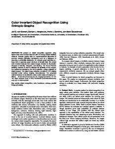
Experiment Setup The data was drawn from a larger study in the Virtual Reality Stroop Task (VRST) [4], where neural and physiological measures were used to predict levels of threat and task difficulty. The VRST is one module in the VRCPAT, a battery of tests found in an adaptive virtual environment, which consists of a virtual city, a virtual vehicle checkpoint, and a virtual Humvee driving scenario in simulated Iraqi and Afghani settings [14]. The VRST involves the subject being immersed in a virtual Humvee that travels down the center of a road in a simulation environment with military relevant events while Stroop stimuli appear on the windshield (see Fig. 2). The VRST is a measure of executive functioning and was designed to emulate the classic Stroop test [15]. Like the traditional Stroop, the VRST requires an individual to press one of three computer keys to identify each of three colors, (i.e., red, green, or blue). Unlike the traditional Stroop, the VRST adds a simulation environment with military relevant events in high and low threat settings. Participants interacted with VRST through an eMagin Z800 head-mounted
(c)
Fig. 2. The Humvee Stroop scenarios. (a) Color naming; (b) Word reading; and, (c) Interference. In this study participants rode in a simulated Humvee through alternating zones of low threat (i.e., little activity aside from driving down a desert road) and high threat (i.e., gunfire, explosions, and shouting amongst other stressors). The VRST was employed to manipulate levels of task difficulty. It consisted of 3 conditions: 1) word-reading, 2) color-naming, and 3) interference. Each Stroop condition was experienced once in a high threat zone and once in a low threat zone. There are many different task difficulty levels in VRST. In this study we chose the following three: • Scenario I: Low threat, color naming. • Scenario II: High threat, color naming. • Scenario III: High threat, interference. Each scenario consisted of 50 stimuli. Three colors (Blue, Green, and Red) were used, and they were displayed randomly with equal probability. In Scenario I, 50 colored numbers were displayed one by one while the subject was driving through a safe zone. Scenario II was similar to Scenario I, except that the subject was driving through an ambush zone. Scenario III was similar to Scenario II, except that Stroop stimuli instead of color naming stimuli were used. In terms of task difficulty, the three scenarios are in the order of I < II < III. A total of 20 college-aged subjects participated in the study. Two of the 20 subjects did not respond at all in one of the three scenarios, and were excluded as outliers. After informed consent was obtained, basic demographic information was recorded. While experiencing the VRST, participant neural and physiological responses – Electrocardiographic activity (ECG),
4
Electrodermal activity (EDA), Electroencephalography (EEG), and Respiration (RSP) – were recorded using a Biopac 150 system. EEG was measured using seven electrodes placed at locations Fp1, Fp2, Fz, Cz, Pz, O1, and O2 according to the international 1020 system for EEG electrode placement. The EEG signal was recorded at 512 Hz, and was referenced to linked ear electrodes. EDA was measured using Ag/AgCl electrodes placed on the index and middle fingers of the non-dominant hand. ECG was recorded with use of a Lead 1 electrode placement, with one Ag/AgCl electrode placed on the right inner forearm below the elbow, another in the same position on the left inner forearm, and a third on the left inner wrist to serve as a ground. Finally, RSP was recorded with a transducer belt placed around widest area of the rib cage. The University of Southern California’s Institutional Review Board approved the study.
R ESULTS Each of the 18 subjects had 150 responses (50 for each task difficulty level). The same 29 features as those in [5] were used to classify the cognitive states, and they are also shown in Table 1. Twenty-one features were extracted from EEG, three from EDA, three from RSP, and two from ECG. Feature extraction consisted of segmenting the data into 3-second epochs that were time locked from 1 second prior to the stimulus occurrence to 2 seconds after. EEG data was filtered using a [1, 30] Hz bandpass filter, epoched into overlapping 1 second windows, and detrended. Spectral power was then calculated in the theta [3.5, 7] Hz, alpha [7.5, 13.5] Hz, and beta [13.5, 19.5] Hz frequency bands for each channel. The EDA features were the mean, minimum, and maximum amplitude response in the epoch window. Respiration was scored similarly, with mean, minimum, and maximum amplitude in the epoch window. ECG features consisted of the number of heartbeats and the average inter-beat intervals (IBIs, scored as the time difference in seconds between successive R waves) in the epoched window. We normalized each feature for each individual subject to [0, 1]. In [5] we have reported that when we trained a SVM classifier on 17 subjects and tested it on the remaining subject, the average classification rate was 36.9%, close to random guess. We also trained a kNN classifier on 17 subjects and tested it on the remaining subject. The average classification rate was 35.8%, again close to random guess. Next we show how classification performance can be improved using our proposed approaches and a few user-specific training examples. In kNN classification we set the maximum number of user-specific training examples to 25, i.e., the algorithms terminated when 25 user-specific training examples were generated. The Euclidean distance was
used. We studied each subject separately, and for each subject l0 = 3 (so that there is at least one user-specific training example for each class). We used li = {1, 2, 3} for ∀i, i.e., in the first experiment, only one userspecific training example was generated in each iteration; in the second experiment, two user-specific training examples were generated in each iteration; and in the third experiment, three user-specific training examples were generated in each iteration. After Iteration i, the kNN classification P performance was i−1 evaluated using the remaining 150− j=0 lj responses from the same subject. We repeated the experiment 100 times (each time the l0 initial training examples were chosen randomly) for each subject and li , and then report the average performances of the four algorithms. It is necessary to repeat the experiment many times to make the results statistically meaningful because there are two forms of randomness: 1) a subject generally had different responses at the same task difficulty level (class label), so for the same sequence of class labels the training examples were different; and, 2) the new class label was generated according to a probability distribution instead of deterministically. The average performances of the four algorithms for li = {1, 2, 3} on the 18 subjects are shown in Fig. 3. The performances on individual subjects are shown in Fig. 4 for li = 1. Observe from Fig. 3 that: 1) T L outperformed the baseline approach. The performance improvement is generally larger when the number of user-specific training examples is small. As the number of user-specific training examples increases, the performances of T L and the baseline converge, i.e. the effect of auxiliary training data decreases as the number of user-specific training data samples increases. 2) ACS outperformed the baseline approach, and when the number of user-specific training examples increased the performance improvement of ACS became larger than the performance improvement of T L over the baseline. 3) T L+ACS outperformed the other three approaches. It inherited both T L’s superior performance for small number of user-specific training examples and ACS’s superior performance for large number of user-specific training examples, and showed improved performance overall. To show that the performance differences among the four algorithms are statistically significant, we performed paired t-tests to compare their average performances, using α = 0.05. The results showed that except for T L+ACS vs ACS for li = 3, the performance difference between all other pair of algorithms is statistically significant (Table 2). As the ultimate goal of the improved algorithms is to learn an optimal classifier using a minimum number of user-specific training examples, it is also interesting to study how many user-specific training
5
TABLE 1 The 29 features used by the kNN classifier. EEG SCL RSP ECG FP1 FP2 Fz Cz Pz O1 O2 SCLmin SCLmax SCLmean RSPmin RSPmax RSPmean Heartbeat IBI θ α β θ α β θ α β θ α β θ α β θ α β θ α β
0.9517
0.9517
0.9517
0.7
0.7558 0.7
0.7313
0.6
0.6
0.5
0.5
0.4 0.3288
0.4 0.3288
0.9517 0.9
0.8
0.9517
0.8
4
10
20
25
0.9517
4
10
20
0.7
0.7702 0.7
0.6
0.6
0.6
0.5
0.5
0.5
0.4 0.3288
0.4 0.3288
0.4 0.3288
25
0.9517
4
10
20
25
0.9517
4
10
20
25
0.9517
0.9517
4
10
20
25
4
10
20
25
4
10
20
25
0.8409 0.8022 0.7
0.6987
0.7
0.6
0.6
0.6
0.6006
0.6444 0.6
0.5
0.5
0.5
0.5
0.5
0.4 0.3288
0.4 0.3288
0.4 0.3288
0.4 0.3288
4
10
20
25
0.9517
4
10
20
25
0.9517
4
10
20
25
0.9517
0.4 0.3288 4
10
20
25
0.9517
0.9517
0.8
0.8
0.7
0.7
0.6
0.6123
0.5974
0.6
0.5425 0.5
0.5
0.5
0.5
0.5
0.4 0.3288
0.4 0.3288
0.4 0.3288
0.4 0.3288
0.4 0.3288
4
10
20
25
0.9517
4
10
20
25
0.9517
0.9517
0.8511 0.8
0.8649 0.8
0.7
0.7
0.661 0.6
0.6
0.6
0.5
0.5
0.5
0.4 0.3288
0.4 0.3288
0.4 0.3288
4
10
20
25
4
10
20
25
4
10
20
25
4
10
20
25
4
10
20
25
Fig. 4. Performance comparison of the four kNN classifiers on the 18 subjects when only one user-specific training example was generated in each iteration. ——: Baseline; – - – -: T L; - - - -: ACS; – – –: T L+ACS.
TABLE 2 Paired t-test results (α = 0.05) for kNN classification. The df for li = 1 is 21 because there are 22 different numbers of user-specific training examples in this case (4, 5, ..., 25). The df for li = 2 is 10 because there are 11 different numbers of user-specific training examples in this case (5, 7, ..., 25). The df for li = 3 is 6 because there are 7 different numbers of user-specific training examples in this case (6, 9, ..., 24).
kNN
li 1 2 3
T L vs Baseline df t p 21 2.66 <0.05 10 3.36 <0.05 6 3.00 <0.05
ACS vs Baseline df t p 21 6.16 <0.05 10 5.62 <0.05 6 5.25 <0.05
T L+ACS vs Baseline df t p 21 7.95 <0.05 10 6.98 <0.05 6 5.69 <0.05
T L+ACS df t 21 9.49 10 8.15 6 7.42
vs T L p <0.05 <0.05 <0.05
T L+ACS vs ACS df t p 21 2.13 <0.05 10 2.69 <0.05 6 2.15 =0.08
6
Classification accuracy
0.76 0.7 0.6 TL+ACS ACS TL Baseline
0.5 0.4 0.3288 4
10
20
25
examples can be saved by using the three improved algorithms, compared with the baseline approach. For each subject, we first find the best performance achieved by the baseline method, which is also the performance when the number of user-specific train′ ing examples is 25. We then find N p , the minimum number of user-specific training examples T L+ACS (or T L, or ACS) needs to achieve the same or better ′ performance. Finally, 25 − N p is the number of userspecific training examples saved by using an improved algorithm. These numbers for the 18 subjects are shown in Fig. 5 for li = {1, 2, 3}. Observe that generally T L can save a small number of user-specific training examples, and the savings of T L+ACS and ACS over the baseline approach are large for most subjects.
Number of user−specific training examples Number of saved examples
(a)
0.7 0.6 TL+ACS ACS TL Baseline
0.4886
0.3288 5
10
20
10 TL+ACS ACS TL
5 0
2
4
6
25
Number of user−specific training examples
(b)
14
16
18
15
10
5
0
TL+ACS ACS TL 2
4
6
8 10 12 Subject index
14
16
18
(b)
0.76 0.7
Number of saved examples
Classification accuracy
8 10 12 Subject index
(a) Number of saved examples
Classification accuracy
0.76
15
0.6 0.5237
TL+ACS ACS TL Baseline
15 10 TL+ACS ACS TL
5 0
2
4
6
0.3288 6
10
20
(c)
Fig. 3. Average performance of the four kNN classifiers on the 18 subjects. (a) One user-specific training example was generated in each iteration; (b) Two userspecific training examples were generated in each iteration; (c) Three user-specific training examples were generated in each iteration.
14
16
18
(c)
24
Number of user−specific training examples
8 10 12 Subject index
Fig. 5. Performance improvements of T L, ACS, and T L+ACS over the baseline approach, in terms of the number of user-specific training examples saved to achieve the best baseline performance. (a) li = 1; (b) li = 2; (c) li = 3.
D ISCUSSIONS We have demonstrated through a kNN classifier that TL and ACS can each help learn an improved classifier given the same number of user-specific training examples, and their combination can achieve even larger performance improvement. So, for same level
7
of classification accuracy, T L+ACS may require a smaller number of user-specific training examples. This will reduce the data acquisition effort to customize an automatic task difficulty recognition system, and hence increase its usability and popularity. Returning to the VE application introduced in the Introduction, here is a scenario of how T L+ACS could be used in automatic cognitive state classification. The VE maintains a database with many different subjects and their physiological responses at different cognitive states. A new user can build his/her profile for automatic cognitive state recognition by taking a few tests online. Assume there are c classes of cognitive states. The VE first displays c tests, one from each class. The physiological responses from the user, along with selected “good” auxiliary training examples from the subject database, are then used by T L to identify the optimal parameters for the classifier. The T L module also computes the classification accuracy from cross-validation using these optimal parameters. If the classification accuracy is not satisfactory, the ACS module then determines from which cognitive class the next test should be displayed. The VE generates the corresponding test and records the user’s physiological responses during the test. Hence a new user-specific training example is obtained and added to the user-specific training example database. The T L module is used again to select the optimal parameters for the classifier and compute the cross-validation accuracy. If the accuracy is satisfactory, then the VE configures the classifier using the optimal parameters and stops training; otherwise, it calls the ACS module to generate another new user-specific training example from the user and iterates the process. The advantage is that, without T L+ACS, the user may need to finish 25 tests to build a reliable classifier, but with T L+ACS, maybe only 15 tests are enough. So, T L+ACS can save the user’s time to customize an automatic cognitive state recognition system. More importantly, this will increase the user’s interest in using such a system, because generally people do not like to take long tests or perform time-consuming calibrations even they are very simple.
C ONCLUSIONS Automatic cognitive state recognition is very important for military training, rehabilitation, soldier safety, and mission success. However, individual differences make it difficult to develop a generic cognitive state recognition algorithm whose model parameters fit all subjects. It is hence important to customize the recognition algorithm for each individual user by adapting its parameters using some user-specific training examples. However, collecting user-specific data is timeconsuming and may also affect the user’s interest in using the recognition system. In this paper we have shown how TL and ACS, and especially their
combination, can help learn an optimal classifier using a minimum number of user-specific (user-specific) training examples. TL exploits the information contained in auxiliary training examples, and ACS optimally selects the new training examples to generate online. Our approaches can reduce the data acquisition effort in customizing a cognitive state recognition system, improving its usability and popularity.
ACKNOWLEDGMENT The data was collected under project “Psychophysiological Interface for Neurocognitive Assessment Using Virtual Environments” W911NF-09-2-0048 (T.D. Parsons, 2009-2012). The research was not supported by any funding.
R EFERENCES 1. 2. 3.
4.
5.
6. 7. 8.
9. 10. 11.
12.
13. 14.
15.
J. Saxton, L. Morrow, A. Eschman, G. Archer, J. Luther, and A. Zuccolotto, “Computer assessment of mild cognitive impairment,” Postgraduate medicine, vol. 121, no. 2, pp. 177–185, 2009. F. D. Rose, B. M. Brooks, and A. A. Rizzo, “Virtual reality in brain damage rehabilitation: Review,” CyberPsychology & Behavior, vol. 8, no. 3, pp. 241–262, 2005. A. Henderson, N. Korner-Bitensky, and M. Levin, “Virtual reality in stroke rehabilitation: A systematic review of its effectiveness for upper limb motor recovery,” Topics in Stroke Rehabilitation, vol. 14, no. 2, pp. 52–61, 2007. T. D. Parsons, C. Courtney, B. Arizmendi, and M. Dawson, “Virtual reality Stroop task for neurocognitive assessment,” Studies in Health Technology and Informatics, vol. 143, pp. 433– 439, 2011. D. Wu, C. G. Courtney, B. J. Lance, S. S. Narayanan, M. E. Dawson, K. S. Oie, and T. D. Parsons, “Optimal arousal identification and classification for affective computing: Virtual Reality Stroop Task,” IEEE Trans. on Affective Computing, vol. 1, no. 2, pp. 109–118, 2010. V. Vapnik, The Nature of Statistical Learning Theory. Berlin: Springer-Verlag, 1995. B. V. Dasarathy, Nearest Neighbor (NN) Norms: NN Pattern Classification Techniques. Los Alamitos, CA: IEEE Computer Society Press, 1991. D. Wu, B. J. Lance, S. S. Narayanan, and T. D. Parsons, “Collaborative filtering for brain-computer interaction using transfer learning and active class selection,” Proc. of the IEEE, 2012, submitted. S. J. Pan and Q. Yang, “A survey on transfer learning,” IEEE Trans. on Knowledge and Data Engineering, vol. 22, no. 10, pp. 1345–1359, 2010. S. Varma and R. Simon, “Bias in error estimation when using cross-validation for model selection,” BMC Bioinformatics, vol. 7, no. 91, 2006. D. Wu and T. D. Parsons, “Inductive transfer learning for handling individual differences in affective computing,” in Affective Computing and Intelligent Interaction, Memphis, TN, October 2011. R. Lomasky, C. E. Brodley, M. Aernecke, D. Walt, and M. Friedl, “Active class selection,” in Proc. 18th European Conference on Machine Learning, Warsaw, Poland, September 2007, pp. 640– 647. D. Wu and T. D. Parsons, “Active class selection for arousal classification,” in Affective Computing and Intelligent Interaction, Memphis, TN, October 2011. T. D. Parsons and A. A. Rizzo, “Affective outcomes of virtual reality exposure therapy for anxiety and specific phobias: A meta-analysis,” Journal of Behavior Therapy and Experimental Psychiatry, vol. 39, pp. 250–261, 2008. J. Stroop, “Studies of interference in serial verbal reactions,” Journal of Experimental Psychology, vol. 18, pp. 643–661, 1935.