PHYSICAL REVIEW B 76, 235326 共2007兲
Current and shot noise in double barrier resonant tunneling structures in a longitudinal magnetic field V. Hung Nguyen and V. Lien Nguyen* Theoretical Department, Institute of Physics, VAST, P.O. Box 429, Bo Ho, Hanoi 10000, Vietnam
T. Anh Pham Physics Faculty, Hanoi National University of Education, 136 Xuan-Thuy, Cau-Giay, Hanoi, Vietnam 共Received 7 March 2007; revised manuscript received 30 August 2007; published 28 December 2007兲 We study the resonant tunneling through double barrier structures in a longitudinal magnetic field. The study shows the necessity of taking into account both the energy dependence and the finiteness of the decay widths of the resonant energy levels, which are closely associated with interesting effects such as the hysteresis, the magnetic-field-induced negative differential conductance, and the shot noise suppression or enhancement. The Landau level quantization produces a strong fluctuation of the noise versus bias at a given magnetic field or the noise versus magnetic field at a given bias. The obtained results provide a better understanding of available experimental data. DOI: 10.1103/PhysRevB.76.235326
PACS number共s兲: 73.40.Gk, 72.70.⫹m, 73.23.⫺b, 75.75.⫹a
The double barrier resonant tunneling structures 共DBRTSs兲 have attracted much attention, both experimental and theoretical, since the original discovery by Tsu and Esaki.1 Besides the very high potential device applications, these structures provide an almost ideal tool for testing different quantum properties of the electron tunneling process. The interest in DBRTSs is related to the very particular current-voltage 共I-V兲 characteristics, which exhibit a strongly superlinear region at relatively low 共preresonant兲 applied bias and a negative differential conductance 共NDC兲 typically accompanied with the hysteresis behavior at higher bias. The hysteresis behavior, observed first by Goldman et al.,2 has been attributed to the intrinsic bistability, which arises from the feedback of the electrostatic potential, induced by the electrons accumulated in the quantum well, on the tunneling current. Such an electron accumulation was also experimentally examined by Young et al.3 and subsequently discussed in Refs. 4–7. Theoretically, the intrinsic bistability observed in I-V curves of DBRTS has been analyzed in a number of works.8–12 Blanter and Büttiker 共BB兲11 have shown that the observed hysteresis behavior is related to the interaction taken into account via the charge accumulated in the well due to capacitive coupling to reservoirs. A magnetic field perpendicular to barriers makes the inplane motion of electrons quantized into Landau levels, and therefore, strongly affects the coupling between the energy levels in the emitter and those in the quantum well. As a result, the I-V curve should have plateaulike features in the preresonant region and the width WB of the bistable region should become field dependent. In reality, such magneticfield related effects have been observed.5,13 Two kinds of AlGaAs-GaAs-AlGaAs DBRTS measured in Ref. 5 correspond to different electron lifetimes in the well, much longer or about the same as the transition time. In the range of magnetic fields ⱕ6 T, while for the former DBRTS the width WB with some fluctuation totally increases, for the latter ones it decreases rapidly and tends to zero, as the magnetic field rises. Theoretically, the magnetic-field effects on the current have been partially described in Ref. 9, where by 1098-0121/2007/76共23兲/235326共7兲
solving self-consistently the Schrödinger and Poisson equations the magnetic-field-induced fluctuation of the width WB as well as of the peak current was qualitatively explained as a direct consequence of the fluctuation of the density of electrons accumulated in the well. While for the current the magnetic-field effect has been widely examined, there are only a few reports on the effect on the shot noise. It is believed that the noise should be even more sensitive than the current to the magnetic field.14 The most interesting experimental data we have found are those reported by Kuznetsov et al. for GaSb-AlSb-InAs-AlSbGaSb DBRTS.15 The main features observed in Ref. 15 are as follows: 共1兲 at zero magnetic field the shot noise is equal to the full shot noise value of 2eI in the low bias region 共where e is the elementary charge and I is the current兲, then becomes significantly suppressed 共sub-Poissonian noise兲, and eventually increases beyond the full shot noise 共superPoissonian noise兲 as the bias increases; 共2兲 the suppression may be as strong as the noise becomes less than half of the full shot noise value; 共3兲 a low magnetic field makes the noise oscillate with bias and the produced noise peaks may exceed the full shot noise value; and 共4兲 the voltages at which the noise peaks occur correspond to the NDC regions in the I-V curve. Theoretically, the suppression and the hysteresis behavior of the shot noise at zero magnetic field have been analyzed in a number of reports.10,11,14,16,18 Actually, the crossover from sub-Poissonian 共in the positive differential conductance region兲 to super-Poissonian shot noise 共in the bistable region兲 in DBRTSs has been predicted by BB.11 Such a crossover is believed to be caused by the Coulomb interaction which affects more the shot noise than the current behavior. Moreover, assuming the decay widths associated with two barriers to be much smaller than all other energy scales in the problem, BB repredicted that the low-limiting value of the noise power spectrum S is half of the full shot noise value.11,17 In other words, following BB the Fano factor, defined as F = S / 2eI, should never be smaller than a half, F ⱖ 1 / 2. Later, Aleshkin et al.18 have claimed that the BB statement of F ⱖ 1 / 2 is, in fact, the consequence of the as-
235326-1
©2007 The American Physical Society
PHYSICAL REVIEW B 76, 235326 共2007兲
NGUYEN, NGUYEN, AND PHAM
sumption on the very small width of the resonant energy level. When this is not the case, calculations18 reveal that the noise power spectrum can be considerably smaller than half the full shot noise value. Note, however, that in Ref. 18 the decay width of the resonant level was taken to be energy independent. Such a simplification may cause a loss of fine structures in the I-V characteristics as well as in the shot noise behavior, and particularly, does not allow us to study adequately the hysteresis behavior.11 Actually, the effect of the magnetic field was not taken into account in both Refs. 11 and 18. The shot noise expression in a longitudinal magnetic field has been derived in Ref. 20, but, as noted by the authors, it is not evident and too complicated to be even qualitatively discussed. The aim of this work is to calculate the current and the shot noise power spectrum in DBRTSs in the presence of a longitudinal magnetic field, taking into account both the energy dependence 共neglected in Ref. 18兲 and the finiteness 共neglected in Ref. 11兲 of the resonant level decay widths. The model under study essentially is an extension of that suggested by BB.11 Besides the quantization of the motion in the longitudinal 共z兲 direction, giving rise to the resonant energy levels En 共n = 0 , 1 , 2 , . . . 兲, the longitudinal magnetic field B causes also Landau quantization of the electron motion in the 共x , y兲 plane. Assuming that the longitudinal and the transverse motions of electrons are separated, the total electron energy measured from the band bottom in the well is given by Enl = En + 共l + 1/2兲c,
n,l = 0,1,2, . . . ,
共1兲
where c = eB / m* is the cyclotron frequency 共the constants ប
right barrier, and L and R are dimensionless parameters. In the following for simplicity we assume that, of all longitudinal energy levels En, only the lowest level E0 is relevant for tunneling, while all other energy levels are much higher. Next, following the work of BB,11 we derive the following expression for the current:
E = E⬜ + Ez ,
D⬜共E⬜兲 = 共m*/2兲 兺 c␦关E⬜ − 共l + 1/2兲c兴,
共3兲
l
which reduces to the standard two-dimensional DOS of D⬜ = m* / 2, when c → 0, and the longitudinal DOS, Dz, in the Breit-Wigner limit is defined as Dz共Ez兲 =
1 ⌫共Ez兲 . 兺 2 n 共Ez − En兲2 + ⌫2共Ez兲/4
⌫L共Ez兲 = L冑Ez共Ez + U − V兲⌰共Ez兲⌰共Ez + U − V兲, ⌫R共Ez兲 = R冑Ez共Ez + U兲⌰共Ez + U兲,
⌫L共Ez兲⌫R共Ez兲 共Ez − E0兲2 + ⌫2/4 共6兲
共7兲
SRR = − SLR = − SRL = SLL , where P1 =
冕
dE⬜D⬜共E⬜兲
冕
dEz
⌫L共Ez兲⌫R共Ez兲 关共Ez − E0兲2 + ⌫2/4兴2
⫻关f L共1 − f R兲 + f R共1 − f L兲兴, P2 =
冕
dE⬜D⬜共E⬜兲
冕
dEz
⌫L共Ez兲⌫R共Ez兲 关共Ez − E0兲2 + ⌫2/4兴2
⫻关⌫R共Ez兲 − ⌫L共Ez兲兴关f L共1 − f R兲 + f R共1 − f L兲兴, P3 =
冕
dE⬜D⬜共E⬜兲
再
⫻ 1−
冕
dEz
⌫L共Ez兲⌫R共Ez兲 关共Ez − E0兲2 + ⌫2/4兴
冎
⌫L共Ez兲⌫R共Ez兲 关f L共1 − f R兲 + f R共1 − f L兲兴. 关共Ez − E0兲2 + ⌫2/4兴 共8兲
In these expressions 共6兲 and 共8兲 f L共R兲 is the Fermi distribution function of the left 共right兲 reservoir. The partial decay widths ⌫L共Ez兲 and ⌫R共Ez兲, following Eq. 共5兲, depend on the voltage drop U. For a given bias V, due to the Coulomb interaction this quantity U should be self-consistently determined from the total charge Q in the quantum well. Denoting the capacitance, associated with the left共right兲 barrier as CL共R兲, the selfconsistent equations for U and Q are given by11 CL共U − V兲 + CRU = eQ, Q = eA
兺
=L,R
冕
dE⬜D⬜共E⬜兲
冕
dEzD共Ez兲f 共Ez + E⬜兲, 共9兲
where A is the structure area in the 共x , y兲 plane, DL共R兲共Ez兲 is the partial longitudinal DOS associating with only the left 共right兲 barrier, i.e., Dz共Ez兲 = DL共Ez兲 + DR共Ez兲, and D共Ez兲 = 关⌫共Ez兲/⌫共Ez兲兴Dz共Ez兲,
共5兲
where V ⬅ eV with V being the voltage applied across the structure, U ⬅ eU with U being the voltage drop across the
dEz
SLL = 共e2/兲关⌳L2 P1 + ⌳LP2 + P3兴,
共4兲
Here ⌫共Ez兲 = ⌫L共Ez兲 + ⌫R共Ez兲 is the total decay width of the single resonant level En and ⌫L共R兲共Ez兲 is the partial decay width for tunneling through the left 共right兲 barrier. From the problem of transmission through a single rectangular barrier, we can write11
冕
Moreover, for the zero-frequency shot noise power spectrum, S ⬅ S共0兲 关 , = L , R兴, we get
共2兲
where the transverse DOS, D⬜, in the presence of a magnetic field has the form
dE⬜D⬜共E⬜兲
⫻关f L共Ez + E⬜兲 − f R共Ez + E⬜兲兴.
and the light velocity are set to 1兲. The density of states 共DOS兲 in the well can be factorized as D共E兲 = D⬜共E⬜兲Dz共Ez兲,
冕
e 2
I=
= L,R.
共10兲
The partial decay widths ⌫L共R兲 can be calculated by solving Eqs. 共9兲 and 共5兲 self-consistently.
235326-2
PHYSICAL REVIEW B 76, 235326 共2007兲
CURRENT AND SHOT NOISE IN DOUBLE BARRIER…
The “interaction energy” ⌳L in the noise expression 共7兲 is defined as ⌳L = egLA / 共CL + CR + C0兲 with C0 = −e具Q典 / U and gL = 具IL典 / U, where the average charge 具Q典 and current 具IL典 are given by Eqs. 共9兲 and 共6兲, respectively. The expressions 共6兲 and 共7兲 have been obtained for DBRTSs in a longitudinal magnetic field, taking into account the finiteness of the decay widths. Setting the field to be zero and replacing in expressions above 关共Ez − E0兲2 + ⌫2 / 4兴−2 and 关共Ez − E0兲2 + ⌫2 / 4兴−1 by 4⌫−1␦共Ez − E0兲 and −1 2⌫ ␦共Ez − E0兲, respectively 共implying infinitesimal decay widths兲, these expressions reduce, respectively, to expressions 共10兲 and 共28兲 derived in Ref. 11. Without this approximation, the calculation of both the current I 共6兲 and the shot noise power spectrum S ⬅ SLL 共7兲 must be performed numerically. In order to proceed calculations we have to introduce the following parameters: the capacitances CL and CR associated with the left and right barriers, respectively, the decay width parameters L and R, the resonant energy E0, and the magnetic field, measured by the frequency c. Here, for simplicity we consider only the case of zero temperature and assume that CL = CR ⬅ C and L = R ⬅ . Furthermore, we assume that the Fermi energies EF in the two reservoirs are equal and that E0 ⬎ EF. Then, choosing EF as the unit of energy, the number of device parameters to be considered reduces to three: , E0, and C. Hereafter, the capacitance, the bias, and the current density are measured in units of m*e2A / 2, EF / e, and m*eEF2 / 22, respectively. For a given set of parameters , E0, and C, both the I-V characteristics and the bias dependence of the shot noise power spectrum can be calculated at different magnetic fields. It is worth noting that, while in the framework of the approximation made in Ref. 11 the current and therefore the shot noise can be calculated only in a limiting range of bias, Va ⬍ V ⬍ VU, where Va is defined as Va = 关共CL + CR兲 / CR兴共E0 − EF兲 and VU is the upper voltage boundary of the bistable region 共Va and V*, respectively, in Fig. 4 in Ref. 11兲, in the present calculation, such a restriction is removed. The expressions 共6兲 and 共7兲 adequately give I and S, respectively, as continuous functions of V in a large range of bias, including the region of V ⬍ Va and the region of V ⬎ VU. The calculations focus on magnetic-field effects, though even at zero field, as can be seen in Fig. 1, they may lead for the current as well as the shot noise some results, which cannot be extracted from the models used in Refs. 11 or 18 Figure 1共a兲 presents the I-V characteristics obtained from Eq. 共6兲 in the case of zero magnetic field for devices with different values of the decay width parameter : 0.002 共dashed兲, 0.05 共dotted兲, and 0.1 共solid line兲 共E0 = 1.5 and C = 1兲. It should be noted that, since the current I increases almost linearly with increasing , the figure was made more compact by plotting I / rather than I along the vertical axis. It is evident from this figure that a decrease of leads to not only a reduction of the current, but also an essential increase of the width WB of the bistable region. For the range of parameters analyzed, we found that WB ⬀ − with  ⬇ 0.9. The ideal case of infinitesimal decay widths considered in Ref. 11 corresponds just to the limit of the largest bistable region.
FIG. 1. 共Color online兲 The reduced current I / 共a兲 and the Fano factor F 共b兲 are plotted against the bias V for structures with E0 = 1.5, C = 1, and various : 0.002 共dashed兲, 0.05 共dotted兲, and 0.1 共solid line兲, in the absence of magnetic field. In 共b兲 the minimal values of F, Fmin, are equal to 0.42, 0.46, and 0.51 for structures with = 0.1, 0.05, and 0.002, respectively. The enhanced noise peaks are generally too high to be fully shown in the scale. Inset in 共b兲: F共V兲 curve 共solid line, left axis兲 and corresponding I-V characteristics 共dotted line, right axis兲 are presented on the full scale for the structure of = 0.1 共solid line in the main figure兲.
The role of the decay width parameter is even more profound on the noise behavior as can be seen in Fig. 1共b兲, where the Fano factor F is plotted versus bias for the same current values considered in Fig. 1共a兲. In general, the F共V兲 curves obtained are similar to those reported in the literature.15,16,18 It consists of the two limiting regions of low and high 关V ⬎ VU兴 biases, where F → 1, and an intermediate region, where the noise is first suppressed and then strongly enhanced as the bias increases. In this figure the magnitude of the suppressed as well as the enhanced shot noise is shown to essentially depend on . In the shot noise suppression regime, the study shows a continuous reduction of the minimal value of the suppressed noise, Fmin, with increasing . For large values, Fmin may become smaller than 1 / 2 共see solid and dotted curves for 艌 0.05兲. A rough numerical estimate for the case under study 共E0 = 1.5 and C = 1兲 suggests that to observe a strong noise suppression with Fmin ⬍ 1 / 2, the parameter must be larger than about 0.01. As was mentioned above, the shot noise suppression with Fmin ⬍ 1 / 2 has been already found in the calculation of Ref. 18. This calculation is, however, done in the simple model where the decay widths are assumed to be energy independent. Figure 1共b兲 not only shows the same phenomenon in our model, which takes into account the energy dependence of the decay
235326-3
PHYSICAL REVIEW B 76, 235326 共2007兲
NGUYEN, NGUYEN, AND PHAM
FIG. 2. 共Color online兲 I-V characteristics in the presence of magnetic fields for a structure with = 0.002, E0 = 1.5, and C = 1 关corresponding to the solid curve in Fig. 1共a兲兴. The different curves correspond to c = 0.2 共solid兲, 0.4 共dashed兲, and 0.6 共dotted line兲. Note that the lower voltage boundaries of the bistable regions in all the three curves are practically coincident in the scale.
FIG. 3. 共Color online兲 The reduced current I / in the presence of a magnetic field of c = 0.2 is plotted versus the bias V for structures with different : 0.005 共solid兲, 0.02 共dashed兲, and 0.04 共dotted line兲 共E0 = 1.5 and C = 1兲. Inset: the 共 − c兲-phase diagram for observing NDC. The NDC can be observed only in the region below the straight line, which is a fit to the calculated points.
widths, but also demonstrates how Fmin depends on the decay widths. Moreover, our study also shows an essential sensitivity of Fmin to the energy E0. For a given 共 = 0.1 as an example兲, the value Fmin rises almost linearly with E0 from 0.41 for a device with E0 = 1.5– 0.53 for a device with E0 = 6 共measured from EF兲. Since the value Fmin is very weakly sensitive to the capacitances CL共R兲 ⬅ C, we suggest the following conditions for observing a strongly suppressed noise with Fmin ⬍ 1 / 2: 共i兲 the decay widths must be not very small and 共ii兲 the resonant level E0 must be not very far from EF. This explains why F cannot be smaller than 1 / 2 in the BB model, when the decay width is set to be infinitesimal. Thus, Fig. 1共b兲 confirms the possibility of the Fano factor to be below 1 / 2 as predicted in Refs. 18 and 19, where such a strong noise suppression was also suggested as an indication of coherent versus sequential tunneling transport. For the noise enhancement in the NDC region, on the other hand, the smaller the higher the noise peak becomes. For instance, we show in the inset of Fig. 1共b兲 the F共V兲 curve 共solid line, left axis兲 and the corresponding I-V characteristics 共dotted line, right axis兲 in the full scale for the case of = 0.1 关the same solid I-V curve in Fig. 1共a兲兴. Here it is interesting to note that the Fano factor F reaches a value as high as ⬇5.7, while no hysteresis has been recognized in the I-V curve. This agrees with experimental data reported by Song et al.6 in suggesting that the charge accumulation, not system unstability, is ultimately responsible for the superPoissonian shot noise in the NDC region. We also point out that the results presented in this inset resemble quite well Fig. 2 in Ref. 16. For devices of smaller , as can be seen in Fig. 1共b兲, the noise peaks may be too high and too sharp to be well presented. Let us now discuss the magnetic-field effects. In Fig. 2 we present the I-V characteristics for the same device as that studied in Fig. 1 共dashed curves with = 0.002兲, but for different magnetic fields: C = 0.2 共solid兲, 0.4 共dashed兲, and 0.6 共dotted line兲. Besides the well-known field-induced staircaselike structure in the I-V characteristics, this figure clearly
shows that the differential conductance may even become negative in the plateaulike regions. For a given field the NDC regime becomes stronger at higher biases. On the other hand, comparing the curves corresponding to different fields, we see that the higher the field the sharper the NDC becomes. For the structure under study the magnetic field of c ⬇ 0.6 can be seen as the high limit for examining the effect of interest, when there remains only one field-induced step in the I-V curve. The features in Fig. 2 agree well with experimental data reported in Ref. 13 for GaAs/ AlAs DBRTSs in magnetic field ranging from 2.81 to 7.18 T. It is important to note that such a magnetic-field-induced NDC could not be predicted in the approximation of Ref. 18, when the decay widths ⌫L共R兲 are assumed to be energy independent 共see inset in Fig. 5兲. This approximation, as is well established, could be considered acceptable only at low biases, when the NDC is still too weak to be observed. Another important condition for realizing a magneticfield-induced NDC is related to the decay width . In Fig. 3, we compare the I-V curves for structures with the same E0共=1.5兲 and C共=1兲, but with different : 0.005 共solid兲, 0,02 共dashed兲, and 0.04 共dotted line兲. Here, for the same reason as in Fig. 1共a兲, we also plot I / instead of I. The magnetic field for all curves is the same, c = 0.2. Clearly, an increase of causes a smear of the steplike structure in the I-V curves and, consequently, a gradual disappearance of the NDC regime. A statistical analysis of numerical results for structures with E0 = 1.5, C = 1, and in the range of 0.005艋 艋 0.06 and for magnetic fields in the range of 0.1艋 C 艋 0.5 leads to the 共 − c兲-phase diagram for observing NDC shown in the inset, where the NDC can be observed only in the region below the straight line. According to this diagram, the minimal magnetic field necessary for the NDC to be observed is approximately proportional to the decay width parameter . Note that, even though in our calculations L and R are equal, since the two decay widths ⌫L and ⌫R 共5兲 depend in different ways on not only the energy but also the bias, the structure is, in fact, asymmetric at finite biases. In the present model, when a positive voltage is set on the left reservoir, the
235326-4
PHYSICAL REVIEW B 76, 235326 共2007兲
CURRENT AND SHOT NOISE IN DOUBLE BARRIER…
FIG. 4. Voltage boundaries 共upper VU and lower VD兲 of bistable regions vary with c. The two upper lines describe VU and the two lower describe VD. for two structures with different : 0.002 共solid兲 and 0.05 共dotted line兲 共E0 = 1.5 and C = 1兲.
higher the bias the smaller ⌫L and the larger ⌫R become, leading to a more asymmetric structure. Such a bias-induced asymmetry is, in fact, similar to that observed in quantum dot systems21 and is responsible for the observed NDC. To examine this idea, the structures were made more 共or less兲 asymmetric by reducing L 共or R兲, while keeping R 共or L兲 fixed. Even though not shown, the obtained results indicate an essential enhancement of the NDC when L is reduced from 0.01 共=R兲 to 0.0001, and, on the contrary, a gradual suppression of the NDC when R is reduced. The NDC almost disappears for the less asymmetric structure with R = 0.0001 and L = 0.01. Orellana et al.22 investigated asymmetric DBRTSs, but they did not discuss the NDC. As for the bistable region, a nonmonotonous variation of the width WB with an increase in the magnetic field can be already seen in Fig. 2, where it is clear that WB共C = 0.4兲 ⬍ WB共0.2兲, but WB共0.6兲 ⬎ WB共0.4兲. A more detailed examination is shown in Fig. 4, where the lower and upper voltage boundaries, VD and VU, of bistable regions are plotted against the magnetic field for the two structures with different : = 0.002 共solid lines兲 and 0.05 共dotted lines兲. Obviously, while the lower boundaries VD 共two lower curves兲 are weakly sensitive to the field, the upper ones VU strongly fluctuate. Such a fluctuation is associated with the position of Landau levels, depending on the magnetic field, relative to the fixed position of Fermi level EF. As the magnetic field increases, a local minimum in the VU共C兲 curve appears, when a Landau level is in alignment with EF. In that case 关c共n + 1 / 2兲 = EF兴, the deepest minimum 关c ⬇ 0.66兴 in the VU共C兲 curve in Fig. 4 corresponds to the level of n = 1. The parameters , E0, and C have no direct relation to the minimum positions discussed, though they can strongly affect the magnitude of both voltage boundaries, VD and VU, as can be seen by comparing the solid lines for = 0.002 and the dotted lines for = 0.05. It is worth to mention that the results presented in Fig. 4, on one hand, are very similar to those reported in Ref. 22 and, moreover, in qualitative agreement with the experimental data reported in Ref. 5 On the other hand, they are different from the monotonous reduction of
FIG. 5. Fano factor F 共solid line, right axis兲 and the corresponding current density I 共dotted line, left axis兲 are plotted versus V 共 = 0.005, E0 = 1.5, C = 1, and c = 0.15兲. Inset: the same as in the main figure for a structure with the same E0, C, and c, but with an energy independent decay width, ⌫ = 0.01 关model 共Ref. 18兲兴.
bistable regions reported in Ref. 23 for the case of DBRTSs in a transverse magnetic field. Certainly, the magnetic-field effects observed in the I-V characteristics, especially the NDC, illustrated in Figs. 2 and 3, should have an influence on the voltage dependence of the noise. In Fig. 5 we present the Fano factor F 共solid line, right axis兲 and the corresponding current density I 共dashed line, left axis兲 plotted against the bias V for the structure with parameters given in the figure and for a magnetic field strength, corresponding to c = 0.15. For such a relatively weak field 共see discussions later兲 more plateaulike regions will be produced in the I-V characteristics and therefore more interesting behaviors of the F共V兲 dependence are expected. Actually, Fig. 5 shows a fluctuation of the factor F with typical features resembling quite well those observed in Ref. 15 In particular, the noise fluctuation is so strong that the valleys may be even lower than 0.5, while the peaks may exceed the full shot noise value. Additionally, the voltage positions of shot noise peaks are well correlated to the NDC regions in the I-V curve. Note that along with the I-V characteristics, the F共V兲-dependence behavior strongly depends on device parameters. To obtain the F共V兲 curves shown in Fig. 5 共for = 0.002兲, which may be compared to the experimental data,15 the typical decay width of the resonant level must be small and, certainly, the energy dependence of ⌫L共R兲 共5兲 must be adequately taken into account. To illustrate the importance of taking into account this energy dependence, we plot in the inset the I-V characteristics 共dashed line, left axis兲 and the F共V兲 curve 共solid line, right axis兲 for the same device and field parameters, but with the assumption of a constant 共energy independent兲 decay width of the model.18 Clearly, there is no NDC in the I-V curve and, accordingly, the noise fluctuation is considerably weakened. Finally, in Fig. 6 we show the Fano factor F at a given bias, V = 2, plotted as a function of the magnetic field measured by c for three structures different only by the values of : 0.01 共solid兲, 0.02 共dotted兲, and 0.05 共dashed line兲. For each structure, the most remarkable feature observed is the fluctuation of the normalized noise F as the magnetic field increases. The higher the field, the larger the typical “period” and the fluctuation amplitude become. Such a feature in the
235326-5
PHYSICAL REVIEW B 76, 235326 共2007兲
NGUYEN, NGUYEN, AND PHAM
FIG. 6. 共Color online兲 Fano factor F at a bias V = 2 is plotted versus c for three structures with different : 0.01 共solid兲, 0.02 共dotted兲, and 0.05 共dashed line兲 共E0 = 1.5 and C = 1兲.
F共c兲 curves is a consequence of the fact that an increase in the magnetic field causes, on one hand, a fluctuation of the relative distance between the chosen bias and the center of plateaulike regions that induces a fluctuation of F. On the other hand, as the field increases, an increase of the distance between two adjacent plateaulike regions leads to an increase of both fluctuation characters, the period and the magnitude. In addition, the three curves in Fig. 6 for different show that from these two characters, only the fluctuation magnitude is sensitive to the decay width parameter : it decreases as increases. For the curve corresponding to the largest in the figure 共dashed line兲, the fluctuation is not seen in the low magnetic-field region up to c ⬇ 0.08. This is because to see a fluctuation the magnetic field must be large enough so that c is larger than the decay width of the resonant level. A fluctuation of F versus the magnetic field has been reported in Ref. 24, but for mesoscopic cavities the reported F-fluctuation behavior is different from that in Fig. 6. We emphasize that the results reported here cannot be obtained using the models in Refs. 11 and 18 where, moreover, the effect of magnetic field was not considered. The present results qualitatively describe a number of experiments.5,6,13,15 To make a quantitative comparison we have to determine the device parameters and the magneticfield strength used in the experiments. While the Fermi energy EF is entirely determined by the donor 共acceptor兲 concentration ND共NA兲 in the contacts, the energy E0 mainly depends on the barrier height and the well width. For the AlGaAs-GaAs-AlGaAs DBRTS measured in Ref. 6 with a well of 4 nm width and a donor concentration of ND = 1 ⫻ 1018 cm−3, using the barrier height of 0.31 eV and the electron effective mass of 0.067m0 共m0 is the mass of a free electron兲, we have EF ⬇ 54.3 meV and E0 ⬇ 115 meV. The experimental value E0 / EF ⬇ 2.1 is then falling well within the range of values considered in the calculations above. Furthermore, taking the resonant level decay widths to be ⬇3.5 meV,9 the typical value of the dimensionless parameter
can be roughly estimated as ⬇0.07. With the value of E0 determined, as discussed in Fig. 1, this value of is too large for the hysteresis to be observed. The super-Poissonian noise in the NDC region observed in Ref. 6 has then no clear relation to the bistability. For nanodevices, in general, the super-Poissonian noise is caused by an electron accumulation and it is not necessarily accompanied by a NDC.25 Regarding the magnetic-field strength, for the GaSbAlSb-InAs-AlSb-GaAs DBRTS with NA = 2 ⫻ 1018 cm−3 measured in Ref. 15 the value 0.15 of the dimensionless magnetic-field parameter c discussed in Fig. 5 corresponds to a magnetic field of ⬇7.5 T. This field is not far from those 共3 – 5 T兲 used in the experiment.15 To obtain a realistic picture of the magnetic-field-induced I-V and F共V兲 curves, the field should be chosen appropriately: not too small so that the plateaulike regions in the I-V curve as well as a strong fluctuation in the F共V兲 curve can be clearly seen, but not too large so that several plateaulike regions can be present. It should be mentioned that the noise is more sensitive than the current to the device parameters. For devices with = 0.05, for example, the F共V兲 curves 共not shown兲 are strongly different from that in Fig. 5, independent of the values E0 and C. Actually, for real devices there has certainly a mutual correlation between these parameters, namely, both and E0 are critically related to the height of barriers. In conclusion, we have calculated the current and the shot noise power spectrum based on a simple DBRTS model, introduced originally by BB,11 in the presence of a longitudinal magnetic field, taking into account the finiteness of the resonant level decay widths. The study is focused on the effect associated with the magnetic field and the finite decay widths. The main results obtained are as follows: 共1兲 the hysteresis behavior can be observed only in structures with relatively small decay widths, 共2兲 the suppressed shot noise power spectrum in the preresonant region may be smaller than half the value of the full shot noise if the decay widths are not too small and the resonant level is not too far from the Fermi energy in the reservoirs, 共3兲 the super-Poissonian noise observed in the NDC region is strongly correlated to the decay widths and is not necessarily accompanied by a bistable region, 共4兲 the magnetic field may produce a NDC, which becomes stronger in structures with small decay widths and at higher biases, 共5兲 the magnetic-field-induced fluctuation of the bistable region width is a clear manifestation of the Landau level structure, 共6兲 the magnetic field makes the shot noise strongly fluctuate with the bias, and 共7兲 at a given bias, the shot noise fluctuates with the magnetic field, the higher the field the larger the period and the fluctuation magnitude become. These results shed light on some controversies17,18 about the shot noise behavior and provide a better understanding of available experimental data. This work was supported by the Ministry of Science and Technology 共Vietnam兲 via the Fundamental Research Program 共Project No. 4.023.06兲.
235326-6
PHYSICAL REVIEW B 76, 235326 共2007兲
CURRENT AND SHOT NOISE IN DOUBLE BARRIER…
*Author to whom correspondence should be addressed;
[email protected] 1 R. Tsu and L. Esaki, Appl. Phys. Lett. 22, 562 共1973兲. 2 V. J. Goldman, D. C. Tsui, and J. E. Cunningham, Phys. Rev. Lett. 58, 1256 共1987兲; Phys. Rev. B 35, 9387 共1987兲. 3 J. F. Young, B. M. Wood, G. C. Aers, R. L. S. Devine, H. C. Liu, D. Landheer, M. Buchanan, A. J. SpringThorpe, and P. Mandeville, Phys. Rev. Lett. 60, 2085 共1988兲. 4 J. F. Young, B. M. Wood, H. C. Liu, M. Buchanan, D. Landheer, A. J. SpringThorpe, and P. Mandeville, Appl. Phys. Lett. 52, 1398 共1988兲. 5 C. J. Goodings, H. Mizuta, and J. R. A. Cleaver, J. Appl. Phys. 75, 2291 共1994兲. 6 W. Song, E. E. Mendez, V. V. Kuznetsov, and B. Nielsen, Appl. Phys. Lett. 82, 1568 共2003兲. 7 Z. J. Qiu, Y. S. Gui, S. L. Guo, N. Dai, J. H. Chu, X. X. Zhang, and Y. P. Zeng, Appl. Phys. Lett. 84, 1961 共2004兲. 8 P. L. Pernas, F. Flores, and E. V. Anda, Phys. Rev. B 47, 4779 共1993兲. 9 W. Potz, Phys. Rev. B 41, 12111 共1990兲. 10 A. L. Yeyati, F. Flores, and E. V. Anda, Phys. Rev. B 47, 10543 共1993兲. 11 Ya. M. Blanter and M. Büttiker, Phys. Rev. B 59, 10217 共1999兲. 12 O. A. Tretiakov, T. Gramespacher, and K. A. Matveev, Phys. Rev. B 67, 073303 共2003兲.
13 P.
J. Turley, C. R. Wallis, S. W. Teitsworth, W. Li, and P. K. Bhattacharya, Phys. Rev. B 47, 12640 共1993兲. 14 Ya. M. Blanter and M. Büttiker, Phys. Rep. 336, 1 共2000兲. 15 V. V. Kuznetsov, E. E. Mendez, J. D. Bruno, and J. T. Pham, Phys. Rev. B 58, R10159 共1998兲. 16 G. Iannaccone, G. Lombardi, M. Macucci, and B. Pellegrini, Phys. Rev. Lett. 80, 1054 共1998兲. 17 Ya. M. Blanter and M. Büttiker, Semicond. Sci. Technol. 19, 663 共2004兲. 18 V. Ya. Aleshkin, L. Reggiani, N. V. Alkeev, V. E. Lyubchenko, C. N. Ironside, J. M. L. Figueiredo, and C. R. Stanley, Phys. Rev. B 70, 115321 共2004兲; Semicond. Sci. Technol. 19, 665 共2004兲. 19 V. Ya. Aleshkin, L. Reggiani, and M. Rosini, Phys. Rev. B 73, 165320 共2006兲. 20 Ø L. Bø and Y. Galperin, Phys. Rev. B 55, 1696 共1997兲. 21 H. Nakashima and K. Uozumi, Jpn. J. Appl. Phys., Part 2 34, L1659 共1995兲. 22 P. Orellana, F. Claro, E. Anda, and S. Makler, Phys. Rev. B 53, 12967 共1996兲. 23 A. Yu. Serov and G. G. Zegrya, Appl. Phys. Lett. 87, 123107 共2005兲. 24 P. Marconcini, M. Macucci, G. Iannaccone, B. Pelle, and G. Marola, Europhys. Lett. 73, 574 共2006兲. 25 V. H. Nguyen and V. L. Nguyen, Phys. Rev. B 73, 165327 共2006兲.
235326-7