Coordination and Costly Preference Elicitation in ...

Viewer
Transcript

Coordination and Costly Preference Elicitation in Electronic Markets

A dissertation presented by

Adam Isaac Juda to The Committee on Higher Degrees in Business Studies (Subcommittee on Information, Technology and Management) in partial fulﬁllment of the requirements for the degree of Doctor of Philosophy in the subject of Information, Technology and Management Harvard University Cambridge, Massachusetts May 2007

c 2007 – Adam Isaac Juda All rights reserved.

Professor David C. Parkes

Adam Isaac Juda

Professor Pai-Ling Yin

Ph.D. candidate

Dissertation advisors Professor Barbara J. Grosz Committee member

Coordination and Costly Preference Elicitation in Electronic Markets

Abstract Electronic markets are based on classic market design assumptions that often do not hold. This thesis examines the conﬂict between theory and practice for the class of Vickrey-Clarke-Groves mechanisms (VCG) and the auctions it has inspired in electronic commerce, most notably the iterative auctions found on eBay. VCG mechanisms provide bidders with an optimal strategy to truthfully reveal their valuations to the marketplace, and in so doing VCG mechanisms enable eﬃcient allocations of goods. VCG assumes not only that consumers are able to coordinate themselves to a single market and moment in time when conducting their transactions, but also that consumers can determine and express their valuations at no cost. However, in systems like eBay, bidders and sellers are highly uncoordinated, and the market is iterative because consumers are often assumed in practice not to have a complete sense of their valuation initially, but to incur costs in order to derive better beliefs of their value. iii

The theory-practice conﬂict is investigated through analytic and empirical analyses of three facets of markets and consumers with independent, private valuations. First, an analysis of 1,956 auctions on eBay for a Dell E193FP LCD monitor reveals the extent to which bidders on eBay are successfully handling their lack of coordination, and the extent to which their inability to behave optimally is hampering the eﬃciency of eBay. Many bidders may be experiencing regret with eﬃciency hampered by as much as 7% as a result. Second, the design of a marketplace for uncoordinated consumers is given that provides consumers with an optimal bidding strategy to truthfully reveal their valuation to a bidding proxy. A simulation study demonstrates that this novel marketplace provides greater eﬃciency than eBay, while also increasing seller revenue. Finally, the eﬃciency of the Iterative Combinatorial Exchange (ICE), designed to accommodate bidders with costly value reﬁnement, is compared to that of a sealed-bid VCG-based marketplace, where the amount of value reﬁnement available to bidders is limited. ICE provides more eﬃcient results, but not dramatically so as compared to the VCG-based market.

iv

Contents Acknowledgments

viii

1 Introduction 1.1 Electronic Markets and Automated Agents 1.2 Vickrey-Clarke-Groves (VCG) Mechanisms 1.3 Assumptions of VCG versus Reality . . . . 1.3.1 Coordination . . . . . . . . . . . . 1.3.2 Costly Preference Elicitation . . . . 1.4 Examining Theory versus Practice . . . . . 1.5 Outline of Thesis . . . . . . . . . . . . . .

. . . . . . .

. . . . . . .

. . . . . . .

1 1 3 5 5 8 11 18

2 eBay and the Multiple Copies Problem 2.1 Introduction . . . . . . . . . . . . . . . . . . . . . . . . . . . . . . 2.2 eBay . . . . . . . . . . . . . . . . . . . . . . . . . . . . . . . . . . 2.2.1 The E193FP Monitor Market on eBay . . . . . . . . . . . 2.3 The Multiple Copies Problem and Strategic Bidding Behavior . . 2.3.1 Existence of the Multiple Copies Problem . . . . . . . . . 2.3.2 Strategic Behavior . . . . . . . . . . . . . . . . . . . . . . 2.3.3 Regression Analysis . . . . . . . . . . . . . . . . . . . . . . 2.4 True Regret and Bidder-Observed Regret . . . . . . . . . . . . . . 2.4.1 Deﬁning Regret and Bidder-Observed Regret . . . . . . . . 2.4.2 Identifying Bidder-Observed Regret in the Data . . . . . . 2.4.3 Number Experiencing Bidder-Observed Regret . . . . . . . 2.4.4 Is Regret due to Search Errors or Strategy Errors? . . . . . 2.4.5 Bidder-Observed Regret does not Imply Irrational Bidding 2.5 How Ineﬃcient is eBay? . . . . . . . . . . . . . . . . . . . . . . . 2.5.1 Simple Metrics Demonstrating Ineﬃciency on eBay . . . . 2.5.2 MIP-based Eﬃciency Calculation . . . . . . . . . . . . . . 2.5.3 Eﬃciency Requiring Knowledge of Value . . . . . . . . . . 2.5.4 Haile and Tamer . . . . . . . . . . . . . . . . . . . . . . . 2.5.5 Extending the Methods of Haile and Tamer . . . . . . . .

. . . . . . . . . . . . . . . . . . .

. . . . . . . . . . . . . . . . . . .

19 19 20 21 22 23 24 26 27 27 29 30 30 32 34 35 37 38 39 42

v

. . . . . . .

. . . . . . .

. . . . . . .

. . . . . . .

. . . . . . .

. . . . . . .

. . . . . . .

. . . . . . .

. . . . . . .

. . . . . . .

. . . . . . .

. . . . . . .

2.6

2.7 2.8

2.5.6 Applying Value Estimates to Valuation of Allocation 2.5.7 An Alternative Mapping of Maximum Bids to Values Comparing eBay to Posted Price Equivalents . . . . . . . . . 2.6.1 Best-Case Posted Price Results . . . . . . . . . . . . 2.6.2 Simulated Average-Case Posted Price Results . . . . Related Work . . . . . . . . . . . . . . . . . . . . . . . . . . Conclusion . . . . . . . . . . . . . . . . . . . . . . . . . . . . 2.8.1 Opportunities for Future Work . . . . . . . . . . . .

. . . . . . . .

. . . . . . . .

. . . . . . . .

. . . . . . . .

3 An 3.1 3.2 3.3

Options Based Solution to the Sequential Auction Problem Introduction . . . . . . . . . . . . . . . . . . . . . . . . . . . . . . . Model . . . . . . . . . . . . . . . . . . . . . . . . . . . . . . . . . . The Sequential Auction Problem . . . . . . . . . . . . . . . . . . . 3.3.1 Deﬁning the Sequential Auction Problem . . . . . . . . . . . 3.4 Options Based Scheme . . . . . . . . . . . . . . . . . . . . . . . . . 3.4.1 Retail Sector as Inspiration . . . . . . . . . . . . . . . . . . 3.4.2 Real Options . . . . . . . . . . . . . . . . . . . . . . . . . . 3.4.3 Costless Real Options . . . . . . . . . . . . . . . . . . . . . 3.4.4 The Bidding Proxy . . . . . . . . . . . . . . . . . . . . . . . 3.4.5 Additional Examples of Market and Proxy Behavior . . . . . 3.4.6 Bookkeeping and Matching Observed Winning Prices . . . . 3.5 Complexity Analysis . . . . . . . . . . . . . . . . . . . . . . . . . . 3.5.1 Computational Complexity . . . . . . . . . . . . . . . . . . . 3.5.2 Truthful Bidding to the Proxy Agent . . . . . . . . . . . . . 3.5.3 Competitive Analysis . . . . . . . . . . . . . . . . . . . . . . 3.6 Validating Design for Simple Bidders . . . . . . . . . . . . . . . . . 3.7 Validating Design for Complex Bidders . . . . . . . . . . . . . . . . 3.8 Extensions . . . . . . . . . . . . . . . . . . . . . . . . . . . . . . . . 3.8.1 Buyer Extensions . . . . . . . . . . . . . . . . . . . . . . . . 3.8.2 Seller Extensions . . . . . . . . . . . . . . . . . . . . . . . . 3.9 Related Work . . . . . . . . . . . . . . . . . . . . . . . . . . . . . . 3.10 Conclusion . . . . . . . . . . . . . . . . . . . . . . . . . . . . . . . . 3.10.1 Opportunities for Future Work . . . . . . . . . . . . . . . .

4 ICE and Sealed-Bid Markets when Values are Unknown 4.1 Introduction . . . . . . . . . . . . . . . . . . . . . . . . . . . 4.2 Model . . . . . . . . . . . . . . . . . . . . . . . . . . . . . . 4.2.1 Participants . . . . . . . . . . . . . . . . . . . . . . . 4.2.2 Tree Based Bidding Language . . . . . . . . . . . . . 4.2.3 Belief of Value and Establishing Initial Value Bounds 4.2.4 Belief Reﬁnement . . . . . . . . . . . . . . . . . . . . 4.2.5 ICE and Activity Rules . . . . . . . . . . . . . . . . . vi

. . . . . . .

. . . . . . .

. . . . . . .

. . . . . . .

. . . . . . . .

48 49 51 51 54 56 57 57

. . . . . . . . . . . . . . . . . . . . . . .

60 60 62 64 66 71 71 72 74 74 79 81 83 83 84 88 92 99 109 110 123 126 129 129

. . . . . . .

133 133 136 136 137 141 141 146

4.3

4.4 4.5

4.2.6 Sealed-Bid Marketplace Experiments . . . . . . . . . . . 4.3.1 Experimental Setup . . . 4.3.2 Market Generator . . . . 4.3.3 Experimental Results . . Related Work . . . . . . . . . . Conclusion . . . . . . . . . . . . 4.5.1 Opportunities for Future

. . . . . . . . . . . . . . . . . . . . . . . . . . . . Work

5 Conclusion

. . . . . . . .

. . . . . . . .

. . . . . . . .

. . . . . . . .

. . . . . . . .

. . . . . . . .

. . . . . . . .

. . . . . . . .

. . . . . . . .

. . . . . . . .

. . . . . . . .

. . . . . . . .

. . . . . . . .

. . . . . . . .

. . . . . . . .

. . . . . . . .

. . . . . . . .

154 157 157 158 159 163 164 165 169

A Appendix for Chapter 2 175 A.1 Raw Data Fields . . . . . . . . . . . . . . . . . . . . . . . . . . . . . 175 A.2 Computed Data Fields . . . . . . . . . . . . . . . . . . . . . . . . . . 176 A.3 OLS Regression Data . . . . . . . . . . . . . . . . . . . . . . . . . . . 178 Bibliography

179

vii

Acknowledgments “The quality of a person’s life is in direct proportion to their commitment to excellence, regardless of their chosen ﬁeld of endeavor.” – Vincent Lombardi (1913-1970) The past six years that collectively make up my graduate experience have been phenomenal, and the only thing of which I can be certain is that I will be unable to suﬃciently thank all of the people that have made this experience possible. Within the conﬁnes of Harvard University, I have been blessed with the opportunity to pursue areas of study simply because I wanted to do so. Outside of the ivory tower, I have been blessed with a group of family and friends that make my life both full and fun. Feeling somewhat lost as I approached the end of my time as an undergraduate at Princeton University, I had the opportunity to intern at the Microsoft Corporation in Redmond, Washington. That summer of 2000 proved to be much more than ﬁnding bugs in Oﬃce, as I was able to witness the complexities on the interface of computer science and management, and left that summer suﬃciently fascinated that I knew formal study at that interface was sure to come. Harvard University, in the form of the Harvard Business School and Harvard School of Engineering and Applied Sciences, has provided me much leeway in explorviii

ing this interface as a member of the second cohort in the joint Ph.D. program in Information, Technology and Management. Entering the program with a background that had neither computer science nor management at its core, I had a tremendous amount to learn, and am grateful to all of the faculty at the University whose courses provided the basis of my education here, including Chris Avery, Lars-Erik Cederman, Kip King, H.T. Kung, Michael Mitzenmacher, Nolan Miller and James Stock. As my advisor when I ﬁrst arrived on campus, Lee Fleming took me under his academic wing and will forever be my ﬁrst co-author on my ﬁrst publication.1 While my research agenda took me in a diﬀerent direction, Lee has continued to be an excellent source of advising for me on a variety of issues, and I will be forever thankful for the kind introduction he provided me into the world of academia. I have also learned a tremendous amount from my peers in computer science, management, and the ITM program, and am particularly thankful for the interactions I have had over the years (both of an academic and non-academic nature) with George Batta, Eric Budish, Giro Cavallo, Lyra Colfer, Florin Constantin, Jacomo Corbo, Amanda Cowen, Jerry Kim, Gavi Kohlberg, S´ebastien Lahaie, Ben Lubin, Loizos Michael, Katy Milkman, Ed Naim, Chaki Ng, Jeﬀ Shneidman, Marcin Strojwas, Hassan Sultan, Mark Szigety, Jason Woodard, Feng Zhu and Darren Zinner. The EconCS and ITM seminars both provided me many excellent opportunities over the years to showcase my works in progress and receive constructive feedback, while Janice McCormick and the staﬀ of the HBS Doctoral Programs Oﬃce, as well as Susan Wieczorek in SEAS, provided regular administrative (and emotional) support for navigating much of the red tape that this University seems to produce ad inﬁnitum. 1

Thank you to the Harvard Business Review for liking pretty pictures!

ix

I do not know where to begin in thanking my committee, as whatever words I express are wholly inadequate in expressing my gratitude. Each member of my committee—David, Pai-Ling and Barbara—has played in a diﬀerent way an integral part to my development over the years, with each being valued by me extraordinarily. David C. Parkes, in particular as my chair, has been most generous, meeting with me weekly for literally years. Having taken his CS 286r class twice for a grade and once as an auditor, as well as his CS 309/310 guided study 27 times, this work would not exist without the guidance he has provided me. I hope that the good names of David C. Parkes, Pai-Ling Yin and Barbara J. Grosz are not diminished with the errors that inevitably must remain in this work, which are undoubtedly exclusively my own. Finally, to the Jews, Bostonians and Judas that have managed to preserve just a little bit of sanity in my life, Thank You! Scott Damrauer, Shasa Dobrow, Adam Fagen, Avi Kogan, Amy Lakin, Daniel E. Levenson, Gabi Soble, Jessica Tuchinsky, and a host of others met at Harvard Hillel not only have been great friends, but also have made my mother less nervous about me being a few hundred miles away from her! The ability to completely step away from the sometimes stressful life as a Harvard graduate student can be diﬃcult. Jeﬀ Buchwald, Jason Cayer, Alex Lasky, Dennis Mercier, Peter Owens, Steven Owens, Darrius Sutherland, Daniel Thrasher, and a host of others from the Brilliant Zer0 / Card Dog / VS System / Yu-Gi-Oh! crowd provided an environment where people just wanted to play games and have fun, calming any source of stress I may have built up when experiments failed or counter-examples were developed proving “theorems” false. Last, but certainly not least, is my family. To my aunt Joyce Juda and grandmother Rose Juda, I have

x

been thrilled to live so close to you over these years and just hang out, whether it be going to the movies, services on Rosh Hashanah and Yom Kippur (with obligatory afternoon games of Rummikub), or playing Bingo at Foxwoods. To the Bethlehem crew (i.e., Abba, Emma, Aaron and Tamar), you have been there since the start (though I suppose Aaron is two years short and Tamar four), and hopefully for many years to come. My only wish is to continue making the four of you proud of me as I go forward.

xi

Chapter 1 Introduction

1.1

Electronic Markets and Automated Agents

Electronic markets have generated signiﬁcant new trading opportunities while allowing for the dynamic pricing of goods (Brynjolfsson and Kahin 2000; Brynjolfsson and Smith 2000; Smith et al. 2000). These applications of information systems are used today not only for person-to-person transactions (e.g., auctions), but also increasingly for such business-to-consumer auctions as selling surplus inventory (Lucking-Reiley and Spulber 2001). Indeed, many authors have written about a future in which commerce is mediated by online, automated trading agents (Sandholm and Lesser 1995; Greenwald and Kephart 1999; Anthony and Jennings 2003). A key challenge for systems with automated trading agents is ensuring that users of the system trust the agents working on their behalf (Cassell and Bickmore 2002; Lee and See 2004), which can be particularly diﬃcult as Sanfey et al. (2003) show that users may have diﬀerent beliefs for automated agents than human agents regarding

1

what constitutes acceptable behavior. As one might expect, Parasuraman and Miller (2004) show that users’ trust in an automated system decreases when an automated system is more prone to making mistakes. While Parasuraman and Miller’s study was examining an automated system for detecting airplane malfunctions, their ﬁnding is no less true within automated marketplaces. When the London International Financial Futures Exchange (Liﬀe) intended to introduce automated trading into their marketplace, there was much debate on the topic, so much so that the Financial Times said at the time that “Electronic trading is the biggest single issue to face the futures community today and the industry has long confronted a philosophical split on its merits.”1 A key area of concern in both domains is that users could not be certain that the automated systems would behave “optimally” in all situations. (Of course, part of the debate here must settle the question of what “optimal” means.) Consequently, the decreased level of trust resulted in users in the work of Parasuraman and Miller ignoring the automated system, while the intended users of Liﬀe called for the automated system never to be implemented in the ﬁrst place. However, that these automated systems do not have explicit performance guarantees does not imply that other automated bidding systems cannot be created with such guarantees. One insight oﬀered by mechanism design is that one can seek to design marketplaces that enable the design of optimal automated bidding agents. I next describe one such classic mechanism, Vickrey-Clarke-Groves (Groves 1979), before continuing to question the assumptions made therein. 1

Financial Times. “Liﬀe’s new automated trading system has sparked a debate on automated trading.” November 30, 1989.

2

1.2

Vickrey-Clarke-Groves (VCG) Mechanisms

Within Vickrey-Clarke-Groves (VCG) mechanisms (a survey of which is provided by de Vries and Vohra 2003), a participant is charged the negative impact her presence in the market has on the other participants. VCG mechanisms are suitable when one seeks to design eﬃcient markets in private value environments. Participants have private values when they possess intrinsic worth for items that is independent of the worth others possess, while eﬃcient markets allocate goods such that the summation of value among all participants for the allocation is maximal across all possible allocations. One example of a VCG-based marketplace is the second-price auction, where an auction winner pays the second highest bid the auctioneer receives. Example 1 Consider a seller of an apple with no value for it, and two bidders Alice (whose value for the apple is $10), and Bob (whose value for the apple is $6). Alice will receive the apple and be charged $6 (as her presence in the market prevented Bob from winning the apple, and so Alice has reduced the values other would have by $6), while Bob will receive nothing and be charged $0 (as Alice would receive the apple independent of Bob’s participation in the market). In fact, the payment scheme in VCG is suﬃciently well constructed that participants should truthfully reveal their valuation to the market maker. In Example 1, Alice has been charged the minimal possible value she could have declared within the marketplace while still winning the item. Because bidders have a (weakly) dominant strategy to be truthful, there are two important ramiﬁcations:

3

• The allocation of the VCG mechanism is perfectly eﬃcient: the item goes to the participant with the highest private value. • An automated bidding proxy can play a provably optimal bidding strategy on behalf of the bidder. The second ramiﬁcation is particularly poignant. Users of VCG-based marketplaces with automated bidding agents can trust that their bidding agent will behave optimally on their behalf (provided users are not seeking to behave collusively with other bidders, or engage in other strategic behavior outside of submitting a bid). The VCG mechanism generalizes to complex allocation problems such as combinatorial auctions (in which multiple diﬀerent items are sold simultaneously, with participants bidding on any number of combinations) and multi-unit auctions (in which multiple copies of the same item are auctioned simultaneously). It is perhaps not surprising that VCG can be considered to be the basis on which today’s most well known online auction systems are based. Auctions on eBay2 are primarily for single items, with automated agents bidding on behalf of users. While an auction is open, a bidder provides an automated agent with a ceiling. The agent then observes what the current winning price of the auction is, and if the ceiling it has received from its bidder is greater than that winning price, the agent will submit a bid above the current winning price (where is set by eBay anywhere from cents to dollars depending on the value of the item). Therefore, when an auction ends, the winning bidder will pay a price above the highest ceiling another bidder submitted, and so the outcome of an isolated auction is nearly identical to the outcome of a VCG second-price auction. 2

http://www.ebay.com

4

1.3

Assumptions of VCG versus Reality

However, there are reasons the participants on eBay should not actually truthfully reveal their valuation ceiling to an eBay bidding agent. While each isolated auction resembles a VCG mechanism, the overall eBay marketplace is not a VCG mechanism. In addition, there are a number of modeling assumptions made in the analysis of a VCG mechanism regarding the abilities of the bidding population in developing the proof of optimality that do not hold. One assumption is that bidders possess independent, private valuations. Bidders with private values for goods have an intrinsic worth for items that is independent of the perception of worth that other bidders have for the same objects. The VCG mechanism is not truthful when bidders values are interdependent, as bidders will not truthfully reveal their perceptions of value to their competitors in an eﬀort to improve their position, resulting in bidders overbidding or underbidding. However, even when the private values assumption is valid (as assumed in this thesis), there remain other assumptions which when relaxed make the strategic bidding problem diﬃcult for bidders participating in electronic markets: coordination and costly preference elicitation. I introduce each of these considerations in turn.

1.3.1

Coordination

A standard assumption made in the analysis of VCG is that all market participants are able to coordinate themselves to a single market and moment in time. However, for many reasons, market participants may be unable to coordinate in this way.

5

One coordination issue is timing - not only may consumers not simultaneously appreciate a desire for the same object or an interest in selling the same item, but also consumers may want to explicitly uncoordinate themselves for strategic reasons (Porter 2004; Hajiaghayi et al. 2005; Parkes 2007). As an example, consumers may purchase groceries when their pantries run empty, but heterogeneities in their consumption rates will result in consumers being interested in purchasing groceries at diﬀerent times. Alternatively, consumers may have diﬀerent deadlines by which they are interested in acquiring or selling objects. For example, a child may be interested in acquiring a particular baseball card within the next week or not at all, while an adult baseball card collector may be willing to pursue the item indeﬁnitely. In this latter example, the collector may even try to hide her interest in the card until the child leaves in an eﬀort to acquire the item in a less competitive environment. Another coordination issue is cost - coordinating all consumers (even if they were all simultaneously interested in buying and selling items) may be prohibitively expensive. For example, the coordination costs and computation costs would be prohibitive if all consumers and producers of food had to organize themselves to a single moment in time for conducting their marketplace.

How Coordination is a Problem eBay, the aforementioned marketplace in which individual auctions operate as open VCG mechanisms, is an example of an uncoordinated electronic marketplace. Buyers and sellers arrive and depart eBay continuously, and many items listed in one eBay auction are essentially identical to those in other auctions, especially in the

6

Consumer Electronics category (Gopal et al. 2005), where the sum of all successfully closed listings during 2005 was $3.5B (of $44B in total for all of eBay). I refer to coordination problems like the multiple copies problem and the exposure problem (to be described below) as the sequential auction problem, because they relate to issues with composing strategies across a sequence of multiple auctions (see also Parkes 2003). A signiﬁcant strategic problem that bidders face is how to bid when multiple copies of an item are oﬀered for sale sequentially. For example, Alice may want an LCD monitor, and could potentially bid in either a 1 o’clock or 3 o’clock eBay auction. (Alternatively, Alice may be the head of a procurement oﬃce where she may participate in either this week’s or next week’s supplier auction for one million ball bearings.) Alice would prefer to participate in the auction that will have the lower winning price, but she cannot determine beforehand which auction that will be. As a result, she could end up winning the “wrong” auction. (While economic models of this scenario exist for which there are equilibrium bidding strategies, this thesis demonstrates that such equilibrium behaviors are not played in practice.) Another problem bidders may face is the exposure problem. Exposure problems exist when buyers desire a bundle of goods but may only participate in single-item auctions. Bykowsky et al. (2000) primarily studied the context of simultaneous singleitem auctions. This thesis focuses on the context of sequential single-item auctions, which are noted by Bykowsky et al. (page 213, Footnote 24) as potentially imposing a greater burden on bidders coupled with greater economic ineﬃciencies. Buyers face risk as they must determine with limited information the extent to which they

7

will incorporate into their bid for a single item the synergy value of the bundle to which the item belongs. For example, if Alice values a video game console by itself for $200, a video game by itself for $30, and both a console and game for $250, Alice must determine how much of the $20 of synergy value she might include in her bid when bidding for the console alone. If Alice incorporates some of the synergy value in her bid for a console (e.g., by placing a bid of $210), she may incur a loss if she can not subsequently win the video game for less than $40. Alternatively, by not incorporating synergies into her bids, Alice may forgo an opportunity to acquire surplus. For instance, if Alice does not incorporate synergy into her bid, but could have acquired a console in auction at a price of $205 and a game at a price of $35, she will have done herself a disservice.

1.3.2

Costly Preference Elicitation

Another assumption made in the analysis of the VCG mechanism is that participants are able to determine and express their private valuations at no cost. However, consumers may face diﬃcult strategic decisions if it is in fact costly for them to determine their values, which is possible even when their valuations are private (Compte and Jehiel 2005; Parkes 2005). For example, consider an avid reader who is interested in mystery novels, and discovers that a new one has just been released. Clearly there is some value the reader will derive from reading the novel, but she may not be fully aware exactly how much she would be willing to pay for the novel until she spends some time reading the ﬁrst few pages and is able to determine the speciﬁc value that reading the entire novel will provide her.

8

Alternatively, consider a widget company that is bidding on the rental of trucks to distribute its widgets. While there is a minimal number of trucks required by the widget company to fulﬁll its distribution needs, calculating this minimal number requires solving a hard problem (Sandholm 1993). (In particular, solving this problem is equivalent to solving the NP-complete “Traveling Salesman Problem,” which in the worst case may require eﬀort exponential in the size of the problem to solve.)

How Costly Preference Elicitation is a Problem The primary diﬃculty a consumer faces when it is costly for her to determine her valuations lies in deciding when she should exploit her current beliefs of value and submit a bid, and when she should explore her valuation by bearing additional costs to reﬁne her beliefs of value (Sandholm 2000; Compte and Jehiel 2005; Parkes 2005). For instance, imagine Alice is currently interested in acquiring a widget priced at $8. Alice believes her value for the widget is likely $10, but has not yet read the ﬁne print on the widget which provides details revealing the widget’s actual value (between $2 and $13). Alice estimates it will take her $2 worth of time to read the ﬁne print and identify the exact worth of the widget. Alice faces the following dilemma: 1. If Alice reads the ﬁne print, she will discover one of three things after identifying the true value of the object: • The widget is worth less than $6, Alice will not purchase the object, and Alice has done herself a service, as she will only incur the reading cost of $2, instead of incurring a cost much greater than that had she purchased the widget for $8 only to realize a value much less than that. 9

• The widget is worth between $6 and $8, Alice will not purchase the item, and Alice has done herself a disservice, as she will incur the reading cost of $2, but would have incurred a loss less than $2 had she purchased the object without having read the ﬁne print. • The widget is valued over $8, Alice will purchase the widget, and Alice has done herself a disservice, as she has incurred the reading cost while purchasing the object anyway. 2. If Alice does not read the ﬁne print, she will discover one of two things by purchasing and using the object: • The widget is worth less than $6, and Alice has done herself a disservice, as she would have incurred less of a loss had she read the ﬁne print and not purchased the widget. • The widget is worth more than $6, and Alice has done herself a service, as she was better oﬀ not having incurred the cost of reading the ﬁne print. 3. If Alice does not read the ﬁne print, and does not purchase the item, she will never know if she made the correct decision, but will suspect that she made a mistake as her belief of value is greater than the posted price. Consequently, Alice does not have a dominant purchasing strategy, as any decision she makes may not maximize her realized surplus in comparison to some alternative she had. However, just as in the case with an uncoordinated market, the negative ramiﬁcations of this scenario extend beyond the consumer. Overall eﬃciency can also be negatively impacted when consumers make a bad decision in pursuing items when preferences are costly to reﬁne or discover. 10

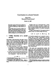
Not Coordinated

Coordinated

Costly Value Determination

Valuation Known at No Cost

eBay

Options Based Marketplace

Iterative Combinatorial Exchange (ICE)

VCG

1

2

3

Figure 1.1: A perspective on the types of populations with independent, private values that various marketplaces are intended to serve, or do serve in practice. While VCG assumes populations are coordinated and able to reﬁne their sense of value for free, the VCG-based eBay marketplace serves consumers who are neither. Highlighted are areas to which this thesis contributes.

1.4

Examining Theory versus Practice

The dilemma examined in this thesis that relates to the place of theoretical assumptions in practical electronic markets is, of course, not new. Marketplaces designed with VCG-based mechanisms and with participants with independent private values may nevertheless still suﬀer from bidding mistakes due to strategic complexities because either participants are uncoordinated or participants cannot reﬁne their value for free. Considering a classiﬁcation of marketplaces by the characteristics of the population it serves or is intended to serve, Figure 1.1 illustrates where markets lie, as well as where this body of work contributes. In three studies, I ask and answer three questions pertaining to academic market assumptions not aligning with realities of user populations:

11

1. To what extent are eBay bidders successfully handling their lack of coordination, and to what extent is their inability to behave optimally hampering eﬃciency? 2. Can one design a marketplace for uncoordinated consumers in which they do have optimal bidding strategies? 3. Is a marketplace designed to accommodate bidders with costly value reﬁnement more eﬃcient than a sealed-bid VCG-based marketplace? Each of these questions is answered in a subsequent chapter of this thesis.

Answering Question 1: eBay and the Multiple Copies Problem eBay provides an excellent example of a marketplace that accommodates a bidding population that is uncoordinated, allowing both buyers and sellers to enter and leave the marketplace continuously. eBay also accommodates a bidding population that possesses costly value reﬁnement processes, allowing bidders to bid multiple times within a given auction. Consequently, a bidder never has to deﬁnitively calculate her true value for an object, but rather must determine only whether her value for a good is above the current winning price within the auction, a less costly act when a bidder can approximate her value but must incur a cost to reﬁne her approximation. However, the manner in which eBay has decided to address the uncoordinated attributes of its bidding population does not provide bidders with optimal bidding strategies; consequently, allocations on eBay may be ineﬃcient. The major contributions of the thesis in this area are • the examination of the extent to which the bidding population on eBay is experiencing regret when pursuing LCD monitors; 12

• the extension of a methodology for approximating an upper bound on the value distribution of eBay bidders based on their observed bidding behavior; and • the estimation of the ineﬃciency on eBay for reasons at least in part attributable to a lack of coordination of the bidding population. I examine the strategic diﬃculties explicitly associated with the bidding population facing multiple auctions that sell the same good, and assume that bidders deﬁnitively know their willingness to pay. At present, uncoordinated consumers who desire items online primarily face two styles of markets, that akin to eBay and that akin to posted price channels such as the online versions of retail stores. Therefore, while eBay may be best suited to a population with costly value reﬁnement, it is reasonable to consider how eﬀective the marketplace is when bidders values are able to be determined at no cost. The analysis will provide a few disturbing results. Signiﬁcant portions of the bidding population may be experiencing regret, and some certainly witness evidence of possible regret. Some bidders appear to be acquiring monitors at prices higher than necessary, while other bidders appear not to be acquiring monitors despite having higher values than other bidders who were present at the same time who do acquire monitors. This latter observation would indicate that the overall eﬃciency of the marketplace is being hampered. While it may not be true in all situations that maximal revenue is achieved when a market is perfectly eﬃcient (Myerson 1981), maximizing the eﬃciency of a system does not have to come at the expense of seller revenue. In fact, Kwasnica et al. (2005) mention that in general the amount of revenue collected is limited by the eﬃciency of

13

the market and that high eﬃciency is coupled with low revenue if and only if bidder proﬁts are high, while high revenue is coupled with low eﬃciency if and only if bidders incur losses. Therefore, in ineﬃcient markets where neither seller revenue is low nor are bidders regularly incurring losses (as is the case on eBay), the ineﬃciencies of the system may be hurting seller revenue. Consequently, improving the allocative eﬃciency of such markets may increase seller revenue.

Answering Question 2: An Options Based Solution to the Sequential Auction Problem Many of the strategic diﬃculties bidders face in markets such as eBay are also faced by consumers acquiring items in the oﬄine retail sector; however, retail stores have developed policies to assist their customers that are facing these problems. Return policies alleviate the exposure problem by allowing customers to return goods at the purchase price. Price matching alleviates the multiple copies problem by allowing buyers to receive from sellers after purchase the diﬀerence between the price paid for a good and a lower price found elsewhere for the same good (Lin 1988; Hess and Gerstner 1991; Chen et al. 2001). With clear means for resolving the core strategic issues facing bidders, these two retail policies provide the basis for a new market scheme - the options based market. The major contributions of the thesis in this area are • the design and analysis of a novel marketplace that explicitly reduces the strategic diﬃculties bidders face when they are uncoordinated, but able to determine their valuation at no cost;

14

• the conducting of simulations of the options based market using a population identical to the estimated eBay population pursuing LCD monitors; and • the conducting of simulations of the options based market for bidding populations with more general valuations. Simulations allow for market to market comparisons of eBay to the options based market, and demonstrate that the options based market outperforms eBay: it generates more revenue in the simulation, and also generates a more eﬃcient allocation of goods. By providing a system in which bidders posses a simple, dominant strategy, sellers reduce the participation costs of bidders. While the magnitude of the eﬀects of reducing these costs is not estimated in this thesis, it can be expected that reducing the participation costs of bidders in the market should both improve bidder loyalty to the sellers and make the market more appealing for new entrants. These two eﬀects ought to preserve and enhance seller revenue in the long term. Corporations would be particularly well suited as users of the options based scheme, as the options based scheme is relevant to all those who sell goods by auction on a regular basis, and could be incrementally implemented as an additional set of rules on top of an existing marketplace. The inclusion of the new rules that would convert a standard sequential auction market to an options based market scheme would be relatively straightforward, and the relationship between sellers and bidders ought to enable such changes in auction policies if so desired by the corporation. Uncoordinated markets selling less traditional goods may also be interested in incorporating the rules to be presented in Chapter 3. There is an ever increasing market

15

for computational services on demand, with computational requirements exceeding locally available resources resulting in universities and institutions requesting services from large collections of intertwined computers, such as grid computing systems like Condor3 and PlanetLab,4 and Amazon.com’s EC25 and S36 web services. As such systems transition to using auctions for acquiring these distributed resources rather than priority systems or ﬁxed prices, the need for mechanisms that can accommodate temporal issues will be ever increasing, and this thesis is relevant for these markets.

Answering Question 3: ICE and Sealed-Bid Markets when Values are Unknown An issue that may be encountered when designing marketplaces is that bidders may be uncertain about their value for goods, particularly if a new type of good is for sale. Not only can determining the values of these new goods be costly, but also these new goods may be only one part of a large and complex valuation, which is private and not interdependent on other bidders’ valuations. Parkes et al. (2005) designed an Iterative Combinatorial Exchange (ICE) to accommodate bidding populations with arbitrarily complex valuations, but uncertainty as to what their speciﬁc valuations on given combinations of goods may be.7 While work to date on ICE (and its tree based bidding language) has focused on the com3

http://www.cs.wisc.edu/condor http://www.planet-lab.org 5 http://aws.amazon.com/ec2 6 http://aws.amazon.com/s3 7 The ICE project began as a class-wide term project in Harvard University’s CS286r during the spring of 2004. Some members of the class, including myself, continued working on the project after the semester, resulting in the work of Parkes et al. (2005) and Cavallo et al. (2005). Ben Lubin, David C. Parkes and I continue to advance the work, currently in the form of Lubin et al. (2007). 4

16

putational eﬃcacy of the exchange, I study for the ﬁrst time not only the eﬃcacy of ICE against a sealed-bid VCG-based marketplace, but also the inﬂuence of costly information revelation. The major contributions of the thesis in this area are • the extension of a value belief system and value reﬁnement process for modeling users of ICE; • the design of an optimal bidding strategy for participants in ICE given a model of costly value reﬁnement; and • the conducting of simulations of the market performance of ICE and sealed-bid markets given identical populations with ﬁnite value reﬁnement budgets. Modeling users as able to reﬁne beliefs about their values but at a cost, I examine the utilities achieved by market participants in ICE compared to market participants who can only submit a single bid in a VCG-based market, limiting the number of the latter populations’ reﬁnements to as many as their respective counterparts make in ICE. In so doing, an evaluation can be made as to whether ICE provides more eﬃcient allocations than VCG-based markets at comparable information revelation costs. Based on simulations, ICE provides more eﬃcient allocations than the VCGbased market. However, the amount by which the allocation is more eﬃcient is small. One area of concern regarding the good performance of the VCG-based market is that bidders’ beliefs may be too accurate because of an artifact in the way that beliefs are modeled. Therefore, I also conduct simulations where the beliefs of bidders are somewhat inaccurate in both ICE and the VCG-based markets. However, comparable results were achieved under these conditions, while the relative performance of ICE increases, the eﬃciency of the VCG-based allocation remains good. 17

1.5

Outline of Thesis

Chapter 2, “eBay and the Multiple Copies Problem,” examines the extent to which bidders on eBay successfully handle their lack of coordination, and to what extent their inability to behave optimally is hampering the eﬃciency of eBay. Chapter 3, “An Options Based Solution to the Sequential Auction Problem,” provides a marketplace design for uncoordinated consumers that provides optimal bidding strategies. Chapter 4, “ICE and Sealed-Bid Markets when Values are Unknown,” examines the eﬃciency of a marketplace designed to accommodate bidders with costly value reﬁnement, comparing it to a VCG-based marketplace. Chapter 5 concludes the thesis. Related work will be discussed toward the end of each chapter.

18

Chapter 2 eBay and the Multiple Copies Problem

2.1

Introduction

Many auctions sell similar items on eBay, raising a series of questions. To what extent do auctions selling similar items interact with each other? To what extent are bidders aware of other auctions selling similar items to the auction in which they are bidding? Do bidders behave in a suﬃciently optimal fashion that they are not experiencing regret? This chapter describes an empirical analysis of the “multiple copies” problem on eBay based on data of bids for 19-inch Dell LCD computer monitors (model E193FP) collected over four months starting in the summer of 2005. Using a conservative model for the arrival and departure time of bidders in the eBay marketplace for LCD screens during this period, this analysis demonstrates that many bidders face multiple

19

auctions selling the same item and that many bidders appear not to secure an optimal result given the sequences of auctions they face. This chapter extends the work of Haile and Tamer (2003) to derive a conservative estimate of the distribution of value of the eBay bidding population for this domain, with the extensions accounting for the multiple copies problem. Using this extended estimate technique, it is possible to approximate how much greater an eBay bidder’s true value is than the maximum bid she was observed to have placed. This estimation can be used to calculate the eﬃciency of eBay, and thus to estimate how ineﬃcient eBay may be for reasons attributed to the multiple copies problem. The calculation shows eBay is 93% eﬃcient with respect to the optimal oﬄine matching that maximizes the total value of goods allocated.

2.2

eBay

eBay is an online marketplace most well known for goods being sold by auction, where thousands of auctions a day are selling a variety of items. Buyers and sellers acquire usernames when they register on eBay (allowing for pseudo-anonymity), and may enter and leave the market dynamically. The most common type of auction held on eBay is a single-item proxy auction. Auctions open at a given time and remain open for a set period of time, usually on the order of days. Potential buyers bid for an item by giving their bidding proxy a value. The proxy will bid on behalf of the buyer only as much as is necessary to maintain a winning position in the auction, up to the value it received from the buyer.

20

Buyers may communicate with the proxy as many times as they wish before the auction closes. Therefore, in the event that a buyer’s proxy has been outbid, a buyer may give the proxy a new, higher value to use in the auction. In essence, eBay implements an incremental version of a Vickrey auction, with the item being sold to the highest bidder for the second-highest bid plus a relatively small increment.

2.2.1

The E193FP Monitor Market on eBay

The market analyzed in this chapter consists of eBay auctions for a speciﬁc LCD computer monitor, a 19” Dell LCD Model E193FP. This market was selected for a variety of reasons including that • the mean closing price of the monitors on eBay is suﬃciently high at $240 with standard deviation $32 that in combination with the typical use of monitors makes it reasonable to assume that bidders are interested in acquiring one copy of the item on eBay;1 • the volume transacted is fairly high, at approximately 500 units sold per month; • the item is not usually bundled with other items in a given auction; and • the item is typically sold as new, so product diﬀerentiation based on quality of the product should not be an issue. Raw auction information was acquired using a PERL script that accesses the eBay search engine,2 and returns all auctions containing the terms ‘Dell’ and ‘LCD’ that have closed within the past month. Data was stored in a text ﬁle for post-processing. 1

For reference, Dell’s October 2005 mail order catalogue quotes the price of the monitor as being $379 without a desktop purchase, and $240 as part of a desktop purchase upgrade. 2 http://search.ebay.com

21

To isolate the auctions in the domain of interest, queries were made against the titles of eBay auctions that closed between 27 May, 2005 through 1 October, 2005. Speciﬁcally, the query found all auctions where the auction title contained all of the following terms: ‘Dell,’ ‘LCD’ and ‘E193FP,’ while excluding all auctions that contained any of the following terms: ‘Dimension,’ ‘GHZ,’ ‘desktop,’ ‘p4’ and ‘GB.’ The exclusion terms exist so that the only auctions analyzed would be those selling exclusively the LCD of interest. For example, the few bundled auctions selling both a Dell Dimension desktop and the E193FP LCD are excluded. Further information on the ﬁelds for each auction and how those ﬁelds were processed is in Appendix A.

2.3

The Multiple Copies Problem and Strategic Bidding Behavior

Analysis of the market shows the following: bidders on eBay face the multiple copies problem, they are as a collective employing several diﬀerent tactics in determining how to bid when facing sequences of auctions, and the results of these tactics seem poor, which may cause problems for sellers as well. Figure 2.1(a) provides a general sense of how the LCD market is shaped, and shows that most auctions close on eBay between noon and midnight EDT, with almost two auctions for the Dell LCD monitor closing each hour on average during peak time periods. The average time a bidder is observed to be in the market is 3.9 days, with a standard deviation of 11.4 days, with Table 2.2(a) providing additional information on the amount of time bidders spent in the market (also referred to as “patience”).

22

4

10

Number of Bidders

Auctions Closing Each Hour

2

1.5

1

0.5

Auctions Available Auctions in Which Bid

3

10

2

10

1

10

0

0 0

5

10

15

Hour of Day

10 0 10

20

1

10

2

10

3

10

Number of Auctions

4

10

(a) The average number of LCD auctions

(b) Histogram of the number of auctions

closing each hour (0 = 00:00 EDT = 12:00AM

available to each bidder and number of auc-

EDT, 15 = 15:00 EDT = 3:00PM EDT)

tions in which a bidder participates.

Figure 2.1: Average number of auctions closing each hour, distribution of number of auctions available to each bidder, and number of auctions in which each bidder bid. This amount of time is calculated as that which passes between when a bidder ﬁrst submits a bid to a bidding proxy and the latest closing time of an auction in which a bidder has participated. Figure 2.1(b) shows how many LCD auctions close while a bidder is in the market.

2.3.1

Existence of the Multiple Copies Problem

While 8,746 bidders (86%) had more than one auction close while they were in the market, with an average of 78 auctions available, only 32.3% of those bidders (27.8% of the bidders in total), are observed to participate in more than one auction. Figure 2.1(b) illustrates the number of auctions in which each bidder participates, with the average bidder particpating in 3.6 auctions.

23

5

Patience 0 sec - 1 hour 6 hours - 1 day 1 day - 7 days 7 days - 30 days More than 30 days

Times Buyer Placed X Bids

10

Count 1589 1151 3731 640 282

4

10

3

10

2

10

1

10

0

10

0

5

10

15

20

25

Number of Bids in an Auction

30

(a) Number of bidders who spend a given

(b) Histogram of number of bids bidders

amount of time in the market attempting to

place in each auction.

acquire an LCD.

Figure 2.2: Information on time bidders spend in market, and histogram of number of bids each bidder places in each auction. The presence of many bids in each auction indicates that no simple strategy is being followed.

2.3.2

Strategic Behavior

The idea that bidders do not act as though each auction has a simple strategy to bid a single time their true willingness to pay is supported by Figure 2.2(b), which shows the frequency of the number of bids bidders place in each auction. If bidders viewed the auctions as being truthful, bidders would only need to place a single bid in any given auction. However, there are many occasions where bidders submit multiple bids to the bidding proxy for a given auction. While 28% of bidders bid in more than one auction, one may wonder the extent to which bidders participate in auctions in sequence, or are simultaneously active in multiple auctions. I deﬁne the activity window of a bidder within an auction as the time from when a bidder ﬁrst places a bid in an auction until the last time in an auction when a bid was provisionally winning (or the end of the auction if the bid24

End

Start

Activity Window

First Bid

Rebid Loses

Immediately Outbid

Range 0.0 - 0.2 0.2 - 0.4 0.4 - 0.6 0.6 - 0.8 0.8 - 1.0

Bids and Wins = time bidder is winning auction

Overlap = 2 Auctions / 3 Total = 0.67

Count 1869 66 153 253 483

(a) Illustrative example deﬁning activity window

(b) Number of bidders with a given over-

and overlap metric for a single bidder bidding in

lap metric among bidders who bid in more

three auctions.

than one auction.

Figure 2.3: Example of overlap metric and histogram of overlap metric among eBay bidding population who bid in more than one auction. There is a large variance in the extent to which bidders are being active in more than one auction simultaneously. While 66% of bidders are active in auctions in a sequential fashion, 26% of bidders are active in multiple auctions simultaneously. der wins the item). For a bidder who bids in multiple auctions, the extent to which activity windows overlap can indicate a relatively complex strategy on the part of a bidder whereby they are particpating back and forth over multiple auctions. I calculate what fraction of a bidder’s activity windows overlap, with Figure 2.3(a) providing a schematic example of how the overlap metric is calculated for a hypothetical bidder who participated in three auctions. Among all bidders that bid in more than one auction, 34.1% had some activity windows overlap. Additionally, of the bidders that bid in more than one auction, 26.1% of them had more than 60% of their activity windows overlapping. This is strong evidence that buyers hop back and forth among auctions, and excercise relatively complex strategies. 25

2.3.3

Regression Analysis

I conduct a simple regression analysis, where the maximal bid submitted by a bidder in an auction is regressed on various aspects of the environment at the time of bidding, including: bidder ﬁxed eﬀects, seller reputation, if the bidder’s activity window in this auction overlapped with the bidder’s activity window in another auction, the total number of opponents who had bid in an auction, the log of time in seconds that a bidder had been in the market, the log of time in seconds remaining in the auction when the bid was placed, and the number of auctions in which a bidder had already bid previously. Table A.1 in Appendix A.3 introduces some summary statistics of these variables as well as the OLS regression-determined values for the coeﬃcients (and errors). There are several interesting statistically signiﬁcant behaviors. Perhaps most relevant in capturing behavior related to the multiple copies problem, bidders tend to submit maximal bids to an auction that are $1.22 higher after spending twice as much time in the system, as well as bids that are $0.27 higher in each subsequent auction. With the amount of time that a bidder has spent in the system being signiﬁcantly correlated statistically to a bidder’s maximum bid in an auction, this may be further evidence that bidders are engaged in a sequential auction bidding strategy. Bidders may be placing bids below their maximum willingness to pay upon entering the market, hoping to win at a low price, and raising their bids closer to their true willingness to pay in auctions over time as they approach their departure from the market. A concern within this dataset is that bidders perceive the value of items as different whereas I assume bidders have comparable value for all items in this dataset.

26

Because the monitors have identical model numbers and are typically sold in brand new condition, there would be no apparent reason for bidders to perceive the objects being sold across auctions as diﬀerent. However, the reputation of sellers does vary from auction to auction, and so could be a cause for bidders to perceive diﬀerent values across auctions (as bidders may believe that sellers with higher reputation are more likely to list honestly an object for sale). However, for this data, there is an absence of statistical signiﬁcance for the impact of a seller’s reputation on the value of bids submitted. Therefore, the statistical results suggest that bidders are not viewing the items in this dataset at heterogeneous.

2.4

True Regret and Bidder-Observed Regret

Because bidders are participating in multiple auctions, often simultaneously, and submitting multiple bids within the auctions in which they participate, this chapter investigates how well bidders actually perform in light of the total number of auctions that were available. In particular, I investigate the extent to which bidders may be experiencing regret.

2.4.1

Deﬁning Regret and Bidder-Observed Regret

I assume bidders are interested in maximizing surplus. In pursuing a single item, a bidder has acquired the maximum possible surplus if she wins a copy of the item at the lowest possible price during the time in which she was in the market, because the value of all monitors in each auction is assumed identical. To do so she must win the auction with the lowest winning price among auctions available. 27

A question arises how to describe a scenario where a bidder wins an item at a price higher than another winning price among the set of auctions she faced (e.g., when a bidder wins an auction at a price of $200, but there was another auction selling an identical item that closed 5 minutes previously for $175). If a winning bidder by bidding diﬀerently would have won another auction at a price below what she paid, securing greater surplus, a bidder is deﬁned as experiencing regret. Deﬁnition 1 (Regret) A bidder experiences regret if she would have been able to realize greater surplus by bidding diﬀerently against the actual bids placed by others in all auctions. However, it is not necessarily true that a bidder has experienced regret when another auction closes for a lower price than what that bidder paid. Consider the following: Example 2 Alice values an apple at $12 and wins Auction B at a price of $10. Alice later observes that Auction A had closed at the same time as Auction B but at a lower price of $7. Unknown to Alice, the winning bid in Auction A was $14. Because the winner of Auction A submitted a winning bid greater than Alice’s value, Alice would not have been able to realize greater surplus by participating in Auction A instead of Auction B (as she only would have raised the price the winner of Auction A would have paid). However, because winning bids are shielded from other participants, Alice is unable to determine when viewing Auction A whether she has experienced regret or not. We deﬁne such a scenario as bidder-observed regret.

28

Deﬁnition 2 (Bidder-observed Regret) A bidder experiences bidder-observed regret when she is unable to prove to herself based on observed information that she has not experienced regret. In essence, a bidder experiences bidder-observed regret if she may have been able to realize greater surplus by bidding diﬀerently, based on the prices she observes of all auctions that were available to her.

2.4.2

Identifying Bidder-Observed Regret in the Data

I identify that bidder-observed regret exists when either of the following two scenarios occurs: 1. A bidder wins an auction at a price higher than the closing price of another available auction. 2. A bidder never wins an auction despite placing a bid in an auction that is higher than the closing price of another available auction. If the winning bidders in all other auctions submitted bids higher than a bidder’s value, the bidder has not experienced regret despite possibly experiencing bidderobserved regret. She neither would have been unable to secure a lower price than the one she realized, nor would ever have been able to win an auction. However, it is true in both instances from the perspective of the bidder that she might have been able to increase her surplus by bidding diﬀerently, and so would experience bidder-observed regret.

29

2.4.3

Number Experiencing Bidder-Observed Regret

Among the 1,817 distinct bidders that won an item via auction, 998 (or 55%) of those bidders won at a price that was higher than the closing price of another auction that closed while the bidder was in the system. This metric is calculated by comparing the price that each winner paid to the minimum closing price among all auctions that were available to the bidder. Furthermore, among the 8,334 bidders that never won an item, 2,708 (or 32%) of those bidders placed a bid higher than the closing price of another auction that closed while the bidder was in the market system. This is calculated by comparing the maximum bid that each non-winning bidder was observed to submit on eBay and comparing it to the minimum closing price among auctions available to the bidder. With more than half of auction winners potentially having been able to do better by winning a diﬀerent auction, and roughly one third of non-winning bidders potentially having been able to win an auction below their losing bids, the current system appears to have opportunities for improvement.3

2.4.4

Is Regret due to Search Errors or Strategy Errors?

As implied by Figure 2.1(b), bidders generally have more auctions available than the number of auctions in which they participated. Table 2.1 shows the number of bidders that participated in all auctions available, for a varying number of auctions. Very few bidders actually participate in all auctions available. Among the 454 bidders that had two auctions available, only 53 bidders (12%) participated in both 3

One area of bias here is the inclusion of buyers at the end of the observation window who may eventually win an auction outside of the observation window. One means to address this concern is to look only at auctions that closed well before the end of the observation window.

30

Table 2.1: Number of bidders who had X auctions available, and the number of bidders who actually participated in all X auctions. Number of auctions, Bidders that had X Bidders who bid in all X % X auctions available auctions that were available 2 454 53 11.67 3 322 1 0.31 4 263 1 0.38 5+ 1785 0 0 auctions; among the 585 bidders that had three and four auctions available, only 2 bidders participated in all auctions available; and among the 1,785 bidders that had ﬁve or more auctions available, no bidders participated in all auctions available. Given that so few bidders are participating in all available auctions, a natural question to ask is, “Should knowing that bidders are not participating in all available auctions change my interpretation of when a bidder experiences regret?” The answer to this question is likely “yes,” particularly if one would like to infer that bidders experiencing regret are making errors in their bidding strategy. There are two diﬀerent ways in which one can interpret a bidder not participating in an auction: 1. A bidder was unaware that the auction existed. While the auction was available in an absolute sense, the auction was not perceived as being available to the bidder, and so a bidder may have never considered the auction when devising her bidding strategy. 2. A bidder was fully aware that the auction existed, but chose not to participate in that auction for strategic reasons. For example, the auction may already have a price higher than a bidder’s maximum willingness to pay, or the bidder may have thought for some reasons that she would not win the auction. 31

Unfortunately, it is impossible to know which scenario exists for any bidder that did not bid in a particular auction without interviewing that bidder. Therefore, while the summary information in Section 2.4.3 is correct when examining all auctions actually available to bidders, it is worth examining how many bidders would experience regret when only considering those auctions in which a bidder actually bid. Among the 508 bidders that won exactly one monitor and participated in multiple auctions, 201 (40%) paid at least $10 more than the closing price of another auction in which they bid, paying on average $35 more (standard deviation $21) than the closing price of the cheapest auction in which they bid but did not win. Furthermore, among the 2,216 bidders that never won an item despite participating in multiple auctions, 421 (19%) placed a losing bid in one auction that was at least $10 higher than the closing price of another auction in which they bid, submitting a losing bid on average $34 more (standard deviation $23) than the closing price of the cheapest auction in which they bid but did not win. Given all the bidder-observed regret demonstrated even when only considering auctions in which a bidder participated, the tie between bidder regret and the strategic decisions (and errors) of bidders appears even stronger.

2.4.5

Bidder-Observed Regret does not Imply Irrational Bidding

While regret may imply that a bidder made a strategic bidding error, a bidder experiencing bidder-observed regret does not imply automatically that a bidder was acting irrationally when bidding. In fact, there are rational explanations for why a 32

bidder would engage in behavior that would result in experiencing bidder-observed regret, and indeed true regret. These reasons get to the heart of the coordination problem present in the eBay market. First, consider the form of bidder-observed regret where a bidder wins an auction at a price higher than the closing price of another available auction. A bidder may rationally bid in a manner that results in this form of bidder-observed regret due to risk aversion. A bidder may observe two auctions, with the ﬁrst auction to close having a higher provisional winning price than the second auction. However, the bidder may choose to bid in the ﬁrst auction for multiple reasons, including: • She may believe the second auction will close at a higher price than at what the ﬁrst auction will close. • She may feel like the risk of skipping the ﬁrst auction and possibly losing the second auction outweighs the risk of possibly paying more in the ﬁrst auction. In both of these situations, a bidder may end up experiencing bidder-observed regret, but would have made a perfectly rational bid at the time when a decision was made. Second, consider the form of bidder-observed regret where a bidder never wins an auction despite placing a losing bid in an auction that is higher than the closing price of another available auction. Again, a rational bid may have been placed that resulted in bidder-observed regret. Example 3 Alice values a monitor at $100, and observes two auctions. Because Alice thinks she ought to be able to win at least one of the auctions with a bid of $80, Alice submits a bid of $80 in the ﬁrst auction to close, losing that auction to someone who bid at least $81. Between the closing of the ﬁrst auction and the second auction, 33

Alice observes the provisional winning price of the second auction at $95, and submits a bid of $100 in an eﬀort to win the item; however, Alice loses that auction at well to someone who bid at least $101. As illustrated in Example 3, Alice experiences bidder-observed regret because she never won an auction despite placing a losing bid of $100 in the second auction that was higher than the $81 closing price in the ﬁrst auction. However, Alice behaved rationally in both auctions given her beliefs. However, bidder-observed regret is still worth measuring, even though bidders experiencing bidder-observed regret may not necessarily have true regret nor have made an irrational bid. Because bidders experience bidder-observed regret (which can be observed) whenever they experience regret (which can not), measuring bidderobserved regret provides an upper bound on how much regret is actually experienced within this bidding population.

Furthermore, a bidder that experiences bidder-

observed regret may also feel as though she has experienced the “winner’s curse,” having paid more for an item than she would have had to otherwise, which increases perceptions of cost of bidding in a marketplace (Bajari and Hortacsu 2003).4

2.5

How Ineﬃcient is eBay?

While Sections 2.4.3 and 2.4.4 demonstrate that many bidders are experiencing bidder-observed regret, it is important to determine the extent to which these errors aﬀect overall market eﬃciency. Eﬃciency, deﬁned as the ratio between the value of 4

I use “winner’s curse” loosely here, as the term normally refers to regret in a common value auction (Krishna 2002).

34

the allocation and the value-maximizing allocation of goods, is an important measure for determining the strength of a market as a whole. When allocative value can be increased, it can be accompanied by increased buyer surplus, increased seller surplus, or both depending on the pricing mechanisms in place. Therefore, determining eﬃciency can be used as a proxy for how competitive a market is in an abstract sense, as an eﬃcient market does not leave the opportunity for another market to simultaneously increase the surplus to both sides of the market; an equally competitive market can only increase bidder surplus by decreasing seller surplus.

2.5.1

Simple Metrics Demonstrating Ineﬃciency on eBay

Fraction of High Bidders among Auction Winners A simple technique for demonstrating ineﬃciency on eBay without explicitly approximating the values bidders have was performed by Gopal et al. (2005) in studying if the auction winners among N auctions were the N highest bidders. They observed that in general not all of the highest bidders were winners of auctions. In my data, given the 1,956 auctions, I ask how many of the 1,956 bidders with the highest bids actually won an auction. The quantity that each eBay bidder is estimated as wanting is the number of times they won an LCD on eBay, or one if they never won an item. Given this, I calculate the fraction of highest-valued bidders that won an auction as the following: j

P ercentW inners = such that

wini ∗ max(1, numW oni ) , (2.1) numAuctions k j = argmax max(1, numW oni ) ≤ numAuctions i=0

k

i=0

35

where wini is a binary variable indicating if bidder i ever won an item, numW oni is the number of monitors bidder i won on eBay, numAuctions is the number of auctions (1956), and where bidders are sorted in decreasing order of maximum bid. The number calculated using this technique, 48.6%, indicates that less than half of the top 1,956 bidders actually won an auction. While this calculation did not include the arrival and departure times of bidders, and so it may be impossible for all 1,956 of the top bidders to win an item in reality due to insuﬃcient temporal supply, this metric still indicates that it is likley that the allocation of goods in practice is not maximizing the value of goods allocated. Therefore, this metric indicates that the market is likley ineﬃcient.

Sum of Closing Prices over Sum of High Bids A simple means for estimating the eﬃciency of eBay is to compare the sum of the 1,956 auction closing prices to the sum of the top 1,956 unique bids submitted: X

P ricei X i=0 j=0 HighBidj

(2.2)

where P ricei is the closing price of auction i, HighBidj is the j’th highest bid, and X is the number of auctions (1,956). Such a calculation has two signiﬁcant omissions. First, such a calculation in no way accounts for the timing eﬀects in the system, it assumes that the bidders are timed in such a fashion that all 1,956 of the top bidders could feasibly win all the monitors. Additionally, eﬃciency is a value metric, while Equation 2.2 is based on prices and bids (although this may be ﬁne if bidders’ values are a constant factor away from the prices and bids observed). However, the equation can provide initial evidence for how ineﬃcient the market may be. 36

The value of this ratio, 90.8% ( $469,821 ), provides evidence that the system is ineﬃ$517,445 cient. Bidders with relatively high bids do not always win auctions, hurting eﬃciency if the auction winners with relatively low bids possess less value than those bidders that do not win auctions but have relatively high bids. While this calculation is a simple estimate, the 9.2% of ineﬃciency calculated is likely not exclusively attributable to the assumptions made in developing this metric.

2.5.2

MIP-based Eﬃciency Calculation

A more accurate calculation for explicitly determining the maximum possible allocation of value, incorporating all timing concerns, can be formulated with a mixedinteger program (MIP). While an oﬄine calculation, the MIP fully conditions for individual bidder’s arrival and departure time in relation to when auctions closed on eBay. Given all bidders, with each bidder i having an arrival time, tai , departure time, tdi , and valuation, vi , and given all auctions, with each auction j having a closing time, tj , the maximum potential allocative value can be calculated by solving the following optimization problem:

37

max

j

i

subject to: a j aji ti j aji tj j aji i aji

vi aji

≤ ≤

j

aji tj , ∀i

j

aji tdi , ∀i

≤1

, ∀i

≤1

, ∀j

aji ∈ {0, 1}

(2.3)

, ∀i, j

where aji is a binary variable which is set to one by the optimization problem if auction j should be allocating its item to buyer i.

2.5.3

Eﬃciency Requiring Knowledge of Value

An obstacle in determining the value of goods allocated on eBay is that I only have access to the bids submitted by bidders, and not the actual values those bidders possess for the items for which they bid. Therefore, I require a methodology for inferring the values bidders possess. Having a method for estimating bidder values comes with multiple beneﬁts. Not only would knowing the values of bidders allow me to determine the value of the allocation of goods on eBay as well as provide an opportunity to analytically calculate the value-maximizing allocation, but also knowing the value of bidders may allow for simulating the bidding population using diﬀerent market mechanisms than that employed by eBay. Because the observed maximum bid that a bidder places on eBay is presumably only a lower bound on the true value that a bidder possesses for the item, a simple 38

ﬁrst order method for recouping the true value bidders have for an item is to multiply bidder i’s observed maximum bid by a constant factor α in order to estimate her true value for the item. For example, if Alice truly values an LCD screen at $330, but only ever placed a bid as high as $300 on eBay, the value of α that would correctly estimate Alice’s true valuation based on her observed maximum bid would be 1.10. In general, one could imagine there being two diﬀerent populations among the bidders for whom one may want to use scaling techniques in an eﬀort to estimate true value based on the observed maximum bid. The ﬁrst population would be eBay winners. Because eBay is a second price auction, I only observe up to the second highest bid received in an auction. Therefore, it is reasonable to believe that winning bidders placed bids that were higher than the winning price by a certain factor. In addition, one could consider scaling all bidders. Because eBay is not a truthful system as a whole, it is quite possible to believe that no bidders submit as their bid their true value, independent of whether they actually win an auction.

2.5.4

Haile and Tamer

In this section, I describe a technique by which one can infer an appropriate value for α. Haile and Tamer (2003) proposed a method for conservatively estimating the bounds of a bidding population’s distribution of value, based on the observed bids that a bidding population makes over a sequence of auctions. Eﬀorts before Haile and Tamer often based their estimations not only on observations of bids placed by bidders in auctions, but also on what were at times strong assumptions of bidding behavior (e.g., assuming that the population was following a certain equilibrium bid-

39

ding strategy). Rather than making a modeling assumption regarding the behavior of bidders, Haile and Tamer use only a “lightweight” set of assumptions when deriving their estimates. 1. Bidders do not bid more than they are willing to pay. 2. Bidders do not allow an opponent to win at a price they are willing to beat. From the ﬁrst of their two assumptions, given the bids placed by each bidder in each auction, Haile and Tamer derive a method for estimating an upper bound of the bidding population’s true value distribution. This value provides a lower bound estimate for the fraction of the population that possesses a value less than a certain amount. From Assumption 2 and the winning price of each auction, Haile and Tamer derive a method for estimating a lower bound of the bidding population’s true value distribution. This value provides an upper bound for what fraction of the population possesses a value less than a certain amount. The estimate of an upper bound is of particular interest in this chapter as it can provide a basis for determining at least how much greater a bidder’s true value is compared to her observed maximum bid. Following Haile and Tamer, I use F (.) to represent the true value distribution of the bidding population, and G(.) the distribution of bids among the bidding population. For an individual bidder, i, bi represents the bid a bidder placed, and vi the bidder’s true value. The ﬁrst of Haile and Tamer’s assumptions implies that bi ≤ vi , ∀i. Therefore G(v) ≥ F (v), ∀v; for at any given value, there are (weakly) more bidders who will bid an amount less than v than there are bidders whose value is truly less than v. Furthermore, within a given auction of n bidders, let bi:n be the i’th lowest bid among the n bids received, while vi:n is the i’th lowest true value 40

among the n bidders. The bidder with the i’th lowest bid does not have to be the same bidder as the one with the i’th lowest true value. The ﬁrst assumption also implies that bi:n ≤ vi:n . One can leverage properties of order statistics established by Arnold et al. (1992) if one assumes that the n bidders in an auction are a random sample of n bidders drawn from the population of eBay participants at large. Given independent and identically distributed random variables {Vi }ni=1 drawn from F(.), the relationship among the distribution of the i’th order statistic of Vi:n , Fi:n (.) and F (.) is as follows: F (v) = φ(Fi:n (v); i, n)

(2.4)

where φ(H; i, n) is bounded between 0 and 1, and can be found by solving the following equation numerically: n! H= (n − i)!(i − 1)!

φ

si−1 (1 − s)n−i ds

(2.5)

0

Haile and Tamer note that while Vi:n cannot be observed, and thus F (.) cannot be inferred from Equation 2.4 directly, one does know the following (from Assumption 1): Fi:n (v) ≤ Gi:n (v), ∀i, n, v

(2.6)

Therefore, Haile and Tamer (2003) Theorem 1 states: F (v) ≤ FU (v) ≡

min n∈[2...M ],i∈[1...n]

φ(Gi:n (v); i, n)

(2.7)

where M is the maximum number of bidders in a given auction. To estimate the upper bound of F (v), FU (v), using ﬁnite observations, one must ﬁrst construct a variable Tn that provides the number of auctions observed with n bidders. From there, one can deﬁne the following empirical distribution: 41

T 1 Gi:n (v) = 1[nt = n, bi:nt ≤ v] Tn t=1

(2.8)

where 1[.] is an indicator function equal to 1 when the argument is true, 0 otherwise. i:n (v), one can estimate the upper bound as: Given G FU (v) ≡

min

n∈[2...M ],i∈[1...n]

i:n (v); i, n) φ(G

(2.9)

With this estimate, Haile and Tamer (2003) develop Theorem 3: For n = 2, ..., M, suppose that Tn → ∞ and Tn /T → λn as T → ∞, with 0 < λn < 1. Then as T → ∞, a.s. FU (v) → FU (v) uniformly in v.

To address small sample bias, Haile and Tamer replace the min function in Equation 2.9 with the following weighted average that approximates the minimum:

µ( y1 , ..., yJ ; ρT ) =

J

exp( yj ρT )

yj J

j=1

yk ρT ) k=1 exp(

(2.10)

y1 , ..., yJ ). where for ρ ∈ , µ( y1 , ..., yJ ; ρT ) > min(

2.5.5

Extending the Methods of Haile and Tamer

The Haile and Tamer estimates are problematic for analyzing eBay for several reasons. In deriving their model of the marketplace, Haile and Tamer assume bidders participate in a single auction. On eBay, as shown in Figure 2.1(b), individual bidders are known to participate in multiple auctions. Furthermore, Haile and Tamer leverage the independence of the bidding population from auction to auction in deriving their estimates. On eBay, it is reasonable to believe that winners of auctions have a relatively lower probability of participating in subsequent auctions, while a losing bidder 42

has a relatively higher probability of participating in subsequent auctions. Therefore, bidding populations are not independent from auction to auction. I extend the work of Haile and Tamer to allow for estimates of the upper bound of the distribution of bidder value despite eBay bidders’ behavior causing many of the assumptions of Haile and Tamer to be invalid. As an illustration of how Haile and Tamer’s methods can be extended, consider the following example: Example 4 On Monday, Alice submits a bid of $50 in an LCD monitor auction that closes on Monday. Alice loses the auction, whereas Bob wins the auction among 8 bidders at a price of $250. On Wednesday, still wanting an LCD monitor, Alice submits a bid of $200 in an auction that closes on Wednesday. Alice loses this auction as well, whereas Charlie wins the auction among 6 bidders at a price of $245. Alice bids in no further auctions. To see how the ﬁrst assumption that Haile and Tamer make can be improved, consider that while it is true that Alice only bid $50 in the Monday auction, I can presume based on her future activity that her true value is not only (weaker) greater than $50, but also (weakly) greater than $200. Therefore, my ﬁrst extension to the work of Haile and Tamer is to make the following assumption to account for bidders participating in multiple auctions: • Within a given auction, each individual bidder’s true value is assumed (weakly) greater than the maximum bid that a bidder submits among all auctions participated (either before or after that auction). Returning to the example, the bidding population is in all likelihood not a true random sampling of the overall population. Those who win auctions are less likely to 43

bid in subsequent auctions, while those who lose auctions are more likely to remain bidders in subsequent auctions as they still demand the item. However, it is not immediately obvious what type of losing bidder is more likely to remain in the system. Low value bidders may ﬁgure they might get lucky if they participate in many subsequent auctions, while high value bidders may believe they are on the verge of winning and so should remain as well. In an eﬀort not to have an individual bidder bias the estimate due to their bidding in multiple auctions, the following adjustment is made to the estimation technique: • If a buyer bids in more than one auction, randomly select one auction in which the bidder bid, and only use that one observation for the estimation. By making this adjustment, the bidders in each auction are unique to that one auction, hence making the bidding observations more appropriate for using the techniques originally suggested by Haile and Tamer. I assume that removing duplicate instances of a bidder is suﬃcient to make the bidding population random over auctions. If one believes that certain portions of the population are drawn to certain auctions, then further adjustments would be required in order to utilize the estimation techniques. Returning to Example 4, when implementing the Haile and Tamer algorithm the following adjustments are made when incorporating Alice into the model: 1. The maximum bid Alice ever submits is $200. Therefore, assume that Alice’s true value is weakly greater than $200. 2. Because Alice bid in two auctions, randomly include her in only one of those auctions for the estimation. Therefore, either: 44

(a) Alice is randomly assigned to the Monday auction, where she is noted as having a value (in eﬀect) of $200 for the purposes of estimating the value distribution. Wednesday’s auction is considered to have only 5 bidders. (b) Alice is randomly assigned to the Wednesday auction, where she is noted as having a value (in eﬀect) of $200 for the purposes of estimating the value distribution. Monday’s auction is considered to have only 7 bidders.

Censoring of Bidders Another concern regarding the bidding population is that there may be a bidder (or many bidders) who would have bid in an auction had the provisionally winning price been below her valuation, but was unable to do so because the price was above her valuation when she found the auction. This censoring of the bidder could be problematic for multiple reasons. First, as the bidder never placed a bid, I would have no way of observing that she “had been” in that auction, resulting in the number of bidders observed as being within that auction being fewer than the total true sample of bidders who observed that auction. Second, because the censored bid is not seen, the eﬀective value of the n’th-highest bidder among all bidders may be diﬀerent. However, the direction of the bias that this censored bid has on my estimate is unclear. In one extreme scenario, a censored bidder may have a value very close to the ﬁnal winning price. Consequently, what I observe to be the third highest bid (and so a lower bound on the third highest value) is actually lower than what the third highest bid could have been. Therefore, the estimation of the upper bound would be further below the distribution of observed bids had the auction observers been incorporated.

45

However, in the alternative extreme scenario, a censored bidder may have a value very close to zero. Consequently, what I observe to be the third highest bid among the N bidders I observe is actually the third highest bid among a number of bidders much greater than that. Therefore, in this scenario, the estimation of the upper bound would be closer to the distribution of observed bids had all bidders who observed the auction been incorporated. Consequently, as censored bidders could be biasing the estimation of the upper bound of value in either direction, I make no corrections in this chapter to try and account for censored bidders.ed the auction been incorporated. Consequently, as censored bidders could be biasing the estimation of the upper bound of value in either direction, I make no corrections in this chapter to try and account for censored bidders.

Applying Extensions to My Data Using the two extensions to the work of Haile and Tamer, I generate estimates of the upper bound of the true valuation distribution using a smoothing parameter value of 1000 (as was done in the original work of Haile and Tamer). I do not consider auctions with more than 17 bidders, as such auctions are suﬃciently rare so as to introduce signiﬁcant small number bias using these estimation techniques. Figure 2.4 displays a variety of distributions of eBay bidders. The “Observed Max Bids” displays the cumulative distribution function (CDF) of bidders’ observed maximum bids on eBay. The “HT upper Bound Est.” displays the estimation of the upper bound of the bidders’ true value distribution based on Haile and Tamer’s algorithm.

46

1

CDF

0.8

Observed Max Bids HT Upper Bound Est. Est. w/ 1st Extension Est. w/ 2nd Extension

0.6 0.4 0.2 0 0

100

200

Value ($)

300

400

Figure 2.4: Cumulative distribution function (CDF) of maximum bids observed, original Haile and Tamer upper bound estimate of bidders’ true value distribution, upper bound estimate incorporating the ﬁrst extension, and upper bound estimate incorporating both extensions. The true value distribution lies (weakly) below the estimated upper bound. The “Est. w/ 1st Extension” displays the results of incorporating the ﬁrst extension to the Haile and Tamer model: acknowledging that the true value a bidder possesses is at least as great as the maximum bid placed among all auctions participated. This adjustment results in the curve being shifted to the right. Such a shift is expected, as each observation of each order statistic is weakly greater after the adjustment than before. However, this extension is not by itself sound because it still leaves in place the bias that I remove with the second extension. The “Est. w/ 2nd Extension” displays the results of my ﬁrst and second extensions: only using each unique bidder in a single auction when estimating the upper bound. These extensions result in a curve between the “HT Upper bound Est.” and the “Est. w/ 1st Extension” curve, and indicates a disproportionate presence of unique high value bidders bidding multiple times in auctions. In the context of these distributions, α is a multiplicative factor which stretches the CDF of maximum bids to the right. Table 2.2 shows the values corresponding 47

Table 2.2: Estimates of the scaling factor, α, from the observed distribution of bids on eBay to the estimated upper bound of true value. An α = 1.42 at the 50th percentile implies that while half of the bidding population placed maximum bids below $180 on eBay, half the population has a true value no less than $255 (42% higher). Percentile ValueObserved ValueEstimate α ≡

Estimate Observed

20th

75

235

3.13

50th

180

255

1.42

80th

240

280

1.17

to the 20th, 50th and 80th percentiles of the distribution functions, as well as the implications for a lower bound of α. At these percentiles the estimates of the lower bound for a value of α vary from 1.17 at higher values (also the observed minimum value among the percentiles) to 3.13 at lower values, indicating that a uniform value for α to be applied to the entire population of 1.15 is reasonably conservative.

2.5.6

Applying Value Estimates to Valuation of Allocation

To estimate the eﬃciency of eBay given the observations, I estimate vi as the maximum observed bid placed by a bidder scaled by α, tai as the time a bidder ﬁrst communicated with an eBay proxy, and tdi as the latest closing time of an auction in which a bidder bid on eBay. Bidders who won more than one item on eBay are cloned so that they appear to be multiple bidders of identical type each wanting one item. While the estimation of the total value allocated to eBay winners is $551,242, the MIP-based calculation (Equation 2.3) estimates that the maximum potential value that could have been allocated is $593,301. Therefore, while the current allocation

48

on eBay appears to be fairly good with respect to allocative value, at 92.9% eﬃcient, there is still a sizeable amount of value not being allocated that could have been, at $42,059. In other terms, while the typical value possessed by a winner on eBay is estimated as $281, an optimal allocation of the goods would have the typical winner possessing a value of $303 for the good. In fact, if one believes that every bidder’s true value is a constant factor α away from their maximum bid, the 92.9% eﬃciency calculation holds for any value of α. However, this belief may not be reasonable, and may alter claims on how eﬃcient the system is. For example, if a bidder on eBay places a bid in a losing eﬀort of $0.50, but truly possesses the highest, unknown value among all bidders, she will not have had her loss properly incorporated into the eﬃciency calculation, introducing upward bias. Alternatively, if losing bidders on eBay tend to have true values close to their observed maximum bids, but eBay winners have true values much greater than their observed maximum bids, then downward bias is introduced in the eﬃciency calculation at present.

2.5.7

An Alternative Mapping of Maximum Bids to Values

While using a constant multiplicative factor of α to transform bids to values enables the eﬃciency estimate of 92.9% to be independent of the exact value of α, I also investigate to what extent the eﬃciency estimate changes if using a non-uniform mapping from bids to values. In particular, I map bids to values according to Table 2.3, adding an amount βi to each bidder’s bid in order to estimate their true value. Bidders whose maximum

49

Table 2.3: Estimates of the additive factor, βi , mapping the observed bid of a bidder on eBay to an estimate of their true value. A βi = 75 at the 50th percentile implies that bidders who were observed to have placed maximum bids on eBay of $180 will be estimated as having true value $75 greater. Percentile ValueObserved ValueEstimate βi = ValueEstimate − ValueObserved 20th

75

235

160

50th

180

255

75

80th

240

280

40

bids are not at these exact percentiles have βi values estimated by linear interpolation.5 This alternative mapping results in the estimated total value allocated to eBay winners being $558,301. (This amount is similar to the previous estimate of $551,242, reﬂecting an oﬀsetting of higher estimated value for low-value winners and lower estimated value for high-value winners.) The MIP-based calculation (Equation 2.3) estimates that the maximum potential value that could have been allocated is $577,615. (This amount is less than the previously estimated $593,301, likely reﬂecting the lower estimates of value for the bidders with the highest of bids.) Therefore, the allocation on eBay using this modiﬁed estimation technique appears to be better than previously estimated, at 96.7% eﬃcient. However, there is still a sizeable amount of value not being allocated that could have been, at $19,314. While the typical value possessed by a winner on eBay is estimatd at $285, an optimal allocation of the goods would have the typical winner possessing a value of $295 for the good. 5

The βi for any bidder below the 20th percentile is estimated as $160, while the βi for any bidder with a maximum bid above $350 is estimated as $0.

50

2.6

Comparing eBay to Posted Price Equivalents

In an eﬀort to further investigate the quality of the eﬃciency claims in Section 2.5.6, I compare eBay to the eﬃciency and revenue that could be generated using a posted-price sales channel, given the same estimated bidding population examined in that section. In particular, I assume a marketplace where for each auction conducted on eBay, a seller will sell their item at a predetermined posted price if there is an interested bidder, rather than conducting an auction for that good.

2.6.1

Best-Case Posted Price Results

As an optimistic assumption, let us assume that the bidders who acquire the items at the posted price are the ones that maximize overall system eﬃciency. With this assumption, the set of bidders who acquire items, as well as the overall system eﬃciency, can be determined using a mixed-integer program very similar to that of Equation 2.3. In particular, Equation 2.3 can be modiﬁed such that the maximum possible allocative value given a posted price, PRICE, is the following:

51

PP Revenue eBay Revenue

2000

PP Value Allocated eBay Value Allocated

1800 Total Items Sold

700000 600000 500000

$

400000 300000 200000 100000

1600 1400 1200 1000 800 600 400 200 0

0 0

100

200

300

400

0

500

100

200

300

400

500

Posted Price ($)

Posted Price ($)

(a) Maximum value allocated and revenue

(b) Total number of items sold in posted

generated in posted price market.

price market.

Figure 2.5: Maximum possible allocative value, revenue and number of items sold in an online posted price marketplace consisting of the eBay buying and selling population.

max

j

i

subject to: a j aji ti j aji tj i aji j aji j aji

vi aji

≤ ≤

j

aji tj , ∀i

j

aji tdi , ∀i

≤1

, ∀j

≤1

, ∀i : vi ≥ PRICE

=0

, ∀i : vi < PRICE

aji ∈ {0, 1}

(2.11)

, ∀i, j

The only diﬀerence between Equations 2.3 and 2.11 is that a buyer is only eligible to be allocated an item if her value for the item is (weakly) greater than the posted price. Figure 2.5(a) shows the maximum possible allocative value and revenues with the population on eBay but using a posted price marketplace, as well as horizontal 52

lines representing the revenue and estimated allocative value of eBay. While revenue initially increases with increasing posted price with no decrease in maximum allocative value possible, both revenue and maximum allocative value possible begin to rapidly decline after a tipping point near a posted price of $275. This can be readily explained by Figure 2.5(b), where the total number of items sold appears to quickly decrease once the posted price is beyond $275. Due to the limited number of people that possess values above those high posted prices, per item revenue increases but not by nearly enough to compensate the reduction in quantity sold. Comparing these data to what actually happened on eBay, posted-price mechanisms have the opportunity to allocate greater value than eBay when the posted price is below $275. This is because it is possible for the posted-price mechanism to achieve perfect eﬃciency in such scenarios. However, as the posted price begins to increase, the number of bidders eligible to purchase items decreases, reducing the maximum possible value of goods allocated beneath that achieved on eBay. Comparing revenue levels, the posted price mechanism achieves generally, but not always, inferior results to eBay. When the posted price is below $250, the revenue generated at each sale prevents it from surpassing the revenue achieved on eBay. Alternatively, when the posted price is above $275, the relatively high revenue per item is oﬀset by the reduced quantity actually sold, resulting in lower overall total revenue. However, at prices between $250-$275, both the revenue achieved in the posted price scheme (as well as the maximum possible allocative value) are superior to that achieved on eBay, conditional on the perfect allocation being achieved.

53

This introduces two interesting lessons regarding the use of a posted price scheme in place of the eBay market as it currently stands. First, a poor selection of a posted price can hamper both system-wide eﬃciency and total seller revenue in comparison to other market mechanisms. Second, an ideal selection of a posted price could achieve both higher total revenue as well as higher value allocated as compared to eBay’s mechanism of holding sequential auctions.

2.6.2

Simulated Average-Case Posted Price Results

I also consider what a more ‘typical’ posted-price result may be rather than the maximum possible result. Rather than using the mixed-integer program of Equation 2.11 to determine the maximum possible value that could be allocated, I instead consider a market where any buyer in the system might obtain the item if they have value beyond the posted price. When an item becomes available at the posted price, a bidder is selected as the winner uniformly at random among all bidders in the system at the time of that sale that possess a value greater than the posted price. Figure 2.6(a) shows the average value allocated and revenues of such an online, posted price marketplace. Similar to Figure 2.5(a), revenue initially increases with increasing posted price, then rapidly declines after a tipping point near a posted price of $250. The slightly earlier tipping point can be explained by comparing Figures 2.5(b) and 2.6(b), where one sees that the total number of items sold decreases sooner in Figure 2.6(b). The trend of allocative value is particularly interesting in 2.6(a). Unlike in Figure 2.5(a), Figure 2.6(a) shows that the total value of goods allocated increases with increasing posted price. This can be explained by viewing the increase

54

PP Revenue eBay Revenue

2000

PP Value Allocated eBay Value Allocated

1800

Total Items Sold

700000 600000 500000

$

400000 300000 200000 100000

1600 1400 1200 1000 800 600 400 200 0

0 0

100

200

300

400

0

500

100

200

300

400

500

Posted Price ($)

Posted Price ($)

(a) Average allocative value and revenue.

(b) Average number of items sold.

Figure 2.6: Average (over 30 simulated runs) of allocative value, revenue and number of items sold in an online posted price marketplace consisting of the eBay population. in posted price as a ﬁltering process whereby low value bidders are excluded from acquiring an item. However, similar to Figure 2.5(a), once the quantity sold begins to decrease, total allocative value decreases. Comparing these data to what actually happened on eBay, Figure 2.6(a) also displays the levels equal to the estimated value allocated on eBay as well as the total revenue achieved on eBay. Comparing allocative value, while Figure 2.5(a) showed that posted price mechanisms could have the opportunity to allocate greater value than eBay, Figure 2.6(a) shows that greater allocative value by the posted price mechanisms is actually not likely in practice as the eligibility for lower valued bidders to acquire items at the posted price reduces the expected allocative value. Similar results appear to be true when comparing revenue. The posted price mechanism achieves inferior revenue results as compared to eBay. With the decrease in items sold occurring earlier in the average-case posted price environment, by the time the per-item revenue is suﬃciently high to possibly exceed eBay, the decrease in quantity sold is too great for the posted price to perform better. 55

This introduces a third interesting lesson regarding the use of a posted price scheme in place of the eBay market. While it is true that an ideal selection of a posted price could achieve both higher total revenue as well as higher allocative value as compared to eBay’s mechanism of holding sequential auctions, it is unlikely that such a result could occur in practice without some other mechanism in place to not only prevent low value bidders from taking advantage of low posted prices, but also having high value bidders win items at the correct times to fully maximize revenue subject to the timing constraints of the bidders.

2.7

Related Work

Shah et al. (2003), Bapna et al. (2004) and Slavova (2006) have developed datadriven approaches toward developing a taxonomy of strategies employed by bidders in practice when facing multi-unit auctions. Unlike their work, this chapter does not aim to classify the various strategies employed by bidders, but rather assess the extent to which bidders are making strategic mistakes whatever their strategy may be. Furthermore, this chapter diﬀers from their work as I am considering the strategic behavior of bidders trying to acquire a single item oﬀered by multiple auctions, while their work considers the strategic behavior of bidders trying to acquire a single item oﬀered by a single multi-unit auction. An alternative approach to the work of Haile and Tamer (2003) for bid identiﬁcation in online auctions has been developed by Jiang and Leyton-Brown (2005) and utilizes machine learning techniques. A signiﬁcant diﬀerence of the work by Jiang and Leyton-Brown is that they generate hidden bids intended to be consistent 56

with the bids observed before computing their maximum-likelihood estimate, whereas Haile and Tamer (and consequently this chapter) base estimates exclusively on the observed bids when generating an upper bound over the unknown, true distribution.

2.8

Conclusion

As many auctions sell similar items on eBay, I study the extent to which bidders appreciate the presence of other auctions when bidding. Conducting an empirical analysis of the “multiple copies” problem on eBay by collecting over four months of bids for computer monitors, I infer a conservative model for the arrival and departure time of bidders in the eBay marketplace for LCD screens during this period. This model demonstrates that many bidders appear to fail in maximizing their surplus given the sequences of auctions they face. I also extend the work of Haile and Tamer (2003) to estimate conservatively the distribution of value of the eBay bidding population for this domain. Based on this extension, I estimate that strategic bidding diﬃculties are contributing to reducing the eﬃciency of the marketplace to 93%.

2.8.1

Opportunities for Future Work

There are a number of interesting extensions that one could pursue in continuing the work of this chapter. Classifying the strategies employed by eBay bidders facing multiple auctions each selling the same item, perhaps extending the work of Bapna et al. (2004), is a worthwhile endevour. Not only would doing so provide additional insight into how users interact with current electronic marketplaces, but also would make it easier to more accurately simulate users within eBay-style markets. 57

Complementary Items Another extension could be to examine a marketplace where bidders desire goods that are complementary, but can only participate in singleitem auctions, and so face the exposure problem. One signiﬁcant obstacle would be in trying to determine how much of a pursued bundle is already held by a bidder before entering the market (e.g., it will be important to have a sound belief as to whether Alice already has or does not have a video game console in her possession when seeing her bidding on a video game). Such an examination would provide valuable insight toward the strategic diﬃculties of current schemes and accompanying ineﬃciencies.

Lab Experiments Lab experiments may provide additional insight into how problematic multiple copies and exposures problems are in practice. By explicitly providing lab participants with their valuation, one could explicitly calculate how many bidders fail to maximize their surplus, explicitly calculate how eﬃcient the experimental marketplace is, explicitly calculate by how much bidders bid below their true values, and conduct surveys to gain insight into why bidders behave as they do.

Validating Haile and Tamer Extensions It would be interesting to validate the appropriateness of the Haile and Tamer extensions through Monte Carlo analysis. Alternatively, in conjunction with lab experiments, one could apply the extended techniques of Haile and Tamer to the bids submitted by lab participants, examining to what extent the extended techniques actually generate conservative bounds of the known true value distribution.

Sniping Finally, an empirical phenomenon observed in this data, and noted before in much literature, is that bidders have a tendency to submit bids toward the end 58

of an auction’s duration. While there are many reasons for bidders to submit bids at the last second, also known as “sniping” (Ockenfels and Roth 2002), this chapter suggests another compelling reason why bidders may snipe even when they possess private valuations. As bidders must consider all auctions they face when trying to maximize their surplus, if a bidder submits a bid to an auction well before an auction closes, they are potentially locking themselves into a bid that would not have been placed conditional on new auctions of which a bidder might become aware between the time at which the bid is placed and when the auction closes. By bidding toward the very end of an auction, a bidder is able to process the best information of both current and future auctions when constructing her bid for the current auction.

59

Chapter 3 An Options Based Solution to the Sequential Auction Problem

3.1

Introduction

I propose a new real options based market infrastructure, coupled with proxy bidding, that enables simple, yet optimal, bidding strategies, while retaining the seller autonomy that is the deﬁning feature of the most successful of today’s open electronic markets, eBay. The options based infrastructure is computationally simple, handles temporal issues, and retains seller autonomy in deciding when to enter the market and conduct individual auctions. The model allows for a market with multiple diﬀerent goods, but assumes that each seller oﬀers a single unit of a good at a time, consistent with common practice on eBay. Bidders may have general valuations on bundles of goods, and the analytic focus of this chapter is for this general model. However, given the prevalence of bidders desiring single items in practice through single item

60

auctions, the empirical focus of this chapter is on bidders who desire a single item and face the multiple copies problem. I do not address the issue of quality of goods, but rather assume that goods can be placed into equivalence classes so that all bidders are indiﬀerent between goods in the same class. A seller allocates an option for her good, which will ultimately either lead to a sale of the good or require that the seller return to the market and oﬀer another option on the same good. Sellers agree to price-match their goods against others of equal type, with the payment a seller ﬁnally receiving deﬁned in terms of the minimal price that the winning bidder could have bid and still traded with a seller in some auction during a bidder’s patience (i.e., the period of time in which a bidder is in the market looking to obtain the item). Bidders must interact through proxy agents, deﬁning a value on all possible bundles of goods in which they have interest. While such an enumeration may seem daunting at ﬁrst glance, there are several reasons not to view this as a major concern. First, a very common purchasing scenario is for a bidder to want a single item, or is indiﬀerent among only a few diﬀerent items. Second, Cantillon and Pesendorfer (2006) provide empirical support that bidders can manage to construct bids in large combinatorial settings. Third, work like that of Cavallo et al. (2005) demonstrates that compact expressions of complete valuations are possible when there exists underlying structure to a valuation. In my proposal, a bidder also declares to her proxy the latest time period in which she is willing to wait to receive the good(s). The proxy agent uses the information about value and patience to determine how much to bid for options, and follows a

61

dominant bidding strategy across all relevant auctions. A proxy agent ﬁnally exercises options held when the bidder’s patience has expired, choosing options that maximize surplus given the reported valuation. All other options are returned to the market and not exercised. The options based protocol makes truthful and immediate revelation to a proxy a dominant strategy for bidders, whatever the future auction dynamics.

3.2

Model

Goods Consider a world with K diﬀerent types of goods G1 ...GK .1 Let T = {0, 1, ...} denote time periods. Let L denote a bundle of goods, represented as a vector of size K, where Lk ∈ {0, 1} denotes the quantity of good type Gk in the bundle. I extend notation whereby a single item k of type Gk refers to a vector L : Lk = 1. Bidders Consider B bidders (sometimes called buyers). The type of a bidder i ∈ B is (ai , di , vi ), with arrival time ai ∈ T , departure time di ∈ T , and private, known, representable valuation vi (L) ≥ 0 for each bundle of goods L received between ai and di , and zero value otherwise. Modeling a bidder’s value as constant during the time in which she is interested in acquiring the bundle is most appropriate when the value of goods will be realized at a speciﬁc moment in time (e.g., Saturday night movie tickets providing a buyer with equivalent value whether they are obtained the prior Monday or Tuesday), or when the range of values for an item is minimal within the 1

A fruit market might sell K=3 types of goods [G1 = apple, G2 = banana, G3 = pomegranate].

62

time period (e.g., an LCD monitor that a buyer plans on using for 3 years provides a buyer with roughly equivalent value if held for 1000 days or 998 days). The arrival time models the period in which a bidder ﬁrst realizes her demand and enters the market, while the departure time models the period in which a bidder loses interest in acquiring the good(s). For example, a bidder may lose interest in an item if a time has passed to acquire an item whose value was realized at a speciﬁc past moment in time (e.g., Saturday night movie tickets providing a buyer no value the following Sunday), or a bidder simply wishes to take advantage of an outside opportunity to acquire the item (e.g., a bidder deciding to acquire an item at a posted price on a certain date if she is unable to secure a better price ﬁrst via an online auction marketplace). In settings with general valuations, I will need an additional assumption (for reasons highlighted in Footnote 4): an upper bound on the diﬀerence between a bidder’s arrival and departure time, denoted ∆Max . While an arbitrarily high ∆Max might be all that can be reasonably assumed in some domains, other domains may lend themselves to lower values. For example, a market maker may be able to determine empirically that buyers interested in acquiring an LCD monitor may always leave the market after unsuccessfully spending no more than one month in the system. Bidders have quasi-linear utilities, so that the utility of bidder i receiving bundle L and paying p, in some period no later than di , is ui(L, p) = vi (L) − p. Sellers Each seller j ∈ S brings a single item kj to the market, has no intrinsic value for the item, and is interested in maximizing revenue. Seller j has an arrival time, aj ,

63

which models the period in which she is ﬁrst interested in listing the item, while the departure time, dj , models the latest period in which she is willing to consider having an auction for the item close. A seller will receive payment at the end of the reported departure of the winning bidder. This model makes no assumption as to when a seller needs to receive the funds for the item sold. While this appears restrictive on the seller, it is not signiﬁcantly diﬀerent than what sellers on eBay currently endure in practice. An auction on eBay closes at a speciﬁc time, but a seller must wait until a bidder relinquishes payment before being able to realize the revenue, an amount of time that could easily be days (if payment is via a money order sent through courier) to much longer (if a bidder is slow but not overtly delinquent in remitting her payment). In this chapter, I assume that sellers are relatively unsophisticated. Without clear incentives to deviate, I assume that sellers will enter the market truthfully.

3.3

The Sequential Auction Problem

In a direct revelation mechanism, each bidder i interacts with the electronic market only once by declaring a bid, bi , which is deﬁned as an announcement of its type, where the announcement may or may not be truthful. I denote all received bids other than i’s as b−i (and at any moment in time, only a subset of these bids may be known to the market as some bids will be received in the future). Given bids, b = (bi , b−i ), the market determines allocations, xi (b), and payments, pi (b) ≥ 0, to each bidder using an online algorithm. Prices are assumed explicitly dependent on the bids (e.g., auctions are not ﬁxed price mechanisms that ignore bids and simply return a constant value for the price). 64

A dominant strategy in this context exists for a bidder if there is a single bid, b∗i , that maximizes the bidder’s utility with respect to all other bids, independent of what other bidders bid. Formally, a dominant strategy equilibrium requires that for each buyer i: ∃b∗i : vi (xi (b∗i , b−i )) − pi (b∗i , b−i ) ≥ vi (xi (bi , b−i )) − pi (bi , b−i ), ∀bi = b∗i , ∀b−i

(3.1)

An auction is deemed strategyproof, when announcing true type is a dominant bidding strategy. As an example, a Vickrey auction (see Vickrey 1961), where a good is allocated to the bidder who submits the highest bid, but the price is the value of the second highest bid, is truthful in isolation. Following Parkes (2003), I deﬁne a locally strategyproof (or truthful) auction, which recognizes participation opportunities in multiple markets, as follows: Deﬁnition 3 Locally strategyproof. An auction is locally strategyproof when truthful bidding is a dominant strategy for a bidder that can only bid in that auction. In practice, there are few instances when a bidder can only participate in a single auction. Generally, such instances occur either because an item for sale is unique and only available for auction once in a bidder’s lifetime (e.g., a unique piece of artwork for which there is no substitute and where the winner of the auction intends to retain ownership forever after), or because a bidder is so impatient in wanting to acquire an item that either she wins the occurring auction for the item or ceases to pursue the item. However, in each of these scenarios, a bidder will have a dominant strategy to bid truthfully provided that the auction is a truthful mechanism.

65

3.3.1

Deﬁning the Sequential Auction Problem

While the discussion in Section 3.2 models what a dominant strategy is in a mechanism where a bidder only makes a single declaration of type, let us now focus on scenarios in practice where bidders must make repeated declarations of type over a sequence of auctions. In this chapter, I focus on the existence (or lack) of strongly dominant strategies (also referred to as “dominant” in this chapter). A strongly dominant strategy will always provide a bidder with (weakly) more surplus than any other strategy no matter the strategies played by other bidders, non-determinism in market clearing rules, or random events that may occur in nature. First, consider the following example in which a bidder does not have a strongly dominant strategy even though each individual auction is locally strategyproof. Example 5 Concrete mixer Alice values acquiring one ton of Sand before Wednesday for $1, 000. Bob will hold a Vickrey auction for one ton of Sand on Monday, and another such auction on Tuesday. In this context, Alice has no dominant bidding strategy. The basic problem is that Alice cannot predict if the price of the Tuesday auction will be greater or less than the price of the Monday auction, which she needs to know when deciding on an optimal bidding strategy on Monday. Example 6 Alice values one ton of Sand with one ton of Stone at $2, 000. Bob holds a Vickrey auction for one ton of Sand on Monday. Charlie holds a Vickrey auction for one ton of Stone on Tuesday.

66

Again, Alice has no dominant bidding strategy because she needs to know the price for Stone on Tuesday in order to know her maximum willingness to pay for Sand on Monday. If Alice bids too high on Monday, she may be left with one ton of Sand but no ability to buy the one ton of Stone required to complete her construction project. If Alice bids too low on Monday, she might forfeit the opportunity to buy both the Sand and Stone despite realizing that she could have aﬀorded to do so after the fact. Deﬁnition 4 The sequential auction problem. Given a sequence of auctions, despite each auction being locally strategyproof, a bidder has no dominant bidding strategy. Consider a sequence of auctions. Assume that a bidder has full knowledge of the rules of the auctions she is about to face, as well as the domain of values of other bidders. Generally, auctions selling the same item will be uncertainly-ordered, because a bidder will not know the ordering of closing prices among the auctions. Deﬁne the interesting bundles for a bidder as all bundles that could maximize the bidder’s proﬁt for some combination of auctions and bids of other bidders (with the empty set being an interesting bundle). Within the interesting bundles, say that an item has uncertain marginal value if the marginal value of an item depends on the other goods held by the bidder. Formally, an item k has uncertain marginal value if the following condition is true: |{m : m = vi (Q) − vi (Q − k), ∀Q ⊆ L ∈ InterestingBundle, Q ⊇ k}| > 1.

(3.2)

Say that an item is over-supplied if there is more than one auction oﬀering an item of that type. Say two bundles are substitutes if one of those bundles has the same value 67

as the union of both bundles. Formally, two bundles A and B are substitutes if vi (A ∪ B) = max(vi (A), vi (B)).

(3.3)

Proposition 1 Given locally strategyproof single-item auctions, the sequential auction problem exists for a bidder if and only if either of the following two conditions is true: (1) within the set of interesting bundles (a) there are two bundles that are substitutes, or (b) there is an item with uncertain marginal value, or (c) there is an item that is over-supplied; (2) a bidder faces competitors’ bids that are conditioned on the bidder’s past bids. Proof. (⇒) By contradiction. Assume the sequential auction problem and that both (1) and (2) are false. If (a) is not true, then the value of a bundle that covers any two interesting bundles is greater than the value of either individual bundle, vi (A ∪ B) > max(vi (A), vi (B)), ∀A, B = φ. Therefore, the bundle containing one copy of each item type Gk must be a bundle strictly valued by the bidder. Formally, a bundle L that is strictly valued has value greater than that implied by free disposal: vi (L) > max vi (Q). Q⊂L

(3.4)

If (b) is not true, then acquiring an additional item, k, of a given type returns the same marginal value, vi (Q) = vi (Q−k)+ck , ∀Q ⊆ L ∈ InterestingBundleSet, Q ⊇ k, where ck is the constant marginal value associated with items of type Gk . Therefore, (a) and (b) both not being true implies that the valuation of any bundle L, must 2 be vi (L) = Therefore, any item k won (up to one copy) k Lk ck by induction. 2

Let M be the maximal bundle covering all interesting bundles, which is strictly valued by the bidder as (a) is not true. As a base case, consider all bundles of size one covered by M , each of

68

below a price of ck increases the proﬁt of the bidder. (c) not being true implies that a bidder would like to win the one auction selling an item if the price is below ck . Therefore, because the auctions are given as locally strategyproof, and by virtue of the bidder not facing competitors’ bids that are conditioned on the bidder’s past bids (i.e., (2) being false by assumption), the bidder has a dominant strategy to bid ck in each auction selling an item of type Gk , which gives a contradiction. (⇐) By case analysis. If (a) is true, then a bidder cannot proﬁtably pursue two bundles at the same time, as she could spend money in acquiring both bundles but not receive value from both. However, a bidder does not know ex-ante which bundle to avoid. Therefore, the bidder does not have a dominant strategy, as ex-post she might win a bundle that she would have been better oﬀ avoiding given the strategies actually played by other bidders.If (b) is true, it is unknown how much to bid on the ﬁrst instance of an item of the given type, as it is unknown which bundle a bidder will eventually win. Therefore, the bidder does not possess a dominant strategy, as ex-post it may be clear that she bid the wrong marginal value for the item given the strategies actually played by other bidders .If (c) is true, given uncertainly-ordered auctions, it is unknown which auction oﬀers the lowest price for some good contained in the bundle that has an over-supplied type. Therefore, there is no dominant strategy, as ex-post a bidder may win the wrong auction selling an item given the strategies actually played by other bidders.If (2) is true, a bidder does not have a dominant strategy as she does not know how to optimally inﬂuence competitors’s bids. which has value ck as (b) is not true. Given bundles of size z covered by M , all bundles of size z + 1 covered by M must be strictly valued as (a) is not true. Each covered bundle of size z + 1, formed by adding k to some covered bundle L of size z, has value vi (L) + ck as (b) is not true. Therefore, by induction, as every bundle L covered by M is constructed by adding each item type Lk times to the empty set, bundle L must have value k Lk ck .

69

As an example, consider a bidder who values one ton of Sand for $1,000, or one ton of Stone for $2,000, but not both Sand and Stone. If the bidder could participate in either a Sand auction or a Stone auction, she faces the sequential auction problem due to condition (a) of Proposition 1 (i.e., Sand and Stone are substitutes, and the bidder might choose the wrong item to pursue). As a second example, consider a bidder who values one ton of Sand for $1,000, and one ton of Sand and one ton of Stone for $1,500. Such a bidder faces the sequential auction problem due to condition (b) of Proposition 1 (i.e., the marginal value for one ton of Sand is uncertain being either $1,000 or $500, and so the bidder might bid the wrong value for Sand in a Sand auction). As a ﬁnal example, consider a bidder who values one ton of Sand for $1,000. If the bidder could participate in more than one auction selling Sand, she faces the sequential auction problem due to condition (c) of Proposition 1 (i.e., there are more auctions selling Sand than quantity demanded by the bidder, and the bidder might not win the cheapest auction available). If a bidder has perfect knowledge about the prices in auctions or that speciﬁc auctions will have a lower or higher price than other auctions, then a bidder may have a dominant strategy and not face the sequential auction problem. For example, if a bidder desires a single item and has two auctions available to her, but the bidder knows that one auction will have a lower closing price, then a bidder may have a dominant strategy to participate in only that lower-priced auction. Alternatively, if a bidder desires a multi-item bundle, and knows how much she will have to spend to win all but one of the items, then the bidder may possess a dominant strategy for bidding for the remaining item the value of the bundle minus the known summation.

70

However, in practice, bidders are regularly arriving and leaving over time and submitting ex-ante unknown bids, with auction prices dependent on those bids. Therefore, a typical bidder will have no means for perfectly knowing the prices they will pay in auctions, or which auctions will have a lower price than other auctions. Subsequently, the assumption of uncertainly-ordered single-item auctions with unknown prices is reasonable in general, thus establishing the sequential auction problem.

3.4 3.4.1

Options Based Scheme Retail Sector as Inspiration

While the Sequential Auction Problem is deﬁned with respect to markets of auctions, many of the meta-strategic problems bidders face are also experienced when consumers try acquire products in the retail sector. The issues around the multiple copies problem are experienced by consumers when multiple stores sell identical products (e.g., eggs, textbooks or shampoo); at any given time, when a consumer is in a store, she can purchase a product at the posted price, but another store might be selling an identical product for a lower price. The issues around the exposure problem can also be experienced; a consumer who wishes to obtain a collection of items at a set budget but must obtain the items at individual stores (e.g., a necktie from one shop and a dress shirt from another) may have to make a purchasing decision without absolute knowledge that she will be able to purchase the necessary complementary items (e.g., she may need to decide whether to purchase a colorful necktie without being certain she will be able to ﬁnd a matching shirt).

71

However, unlike many auctions systems, the retail sector has already developed policies to assist their customers in addressing sequential purchasing problems. Return policies alleviate the exposure problem by allowing customers to return goods at the purchase price without penalty. Additionally, price matching alleviates the multiple copies problem by allowing customers to receive from sellers after purchase the diﬀerence between the price paid for a good and a lower price found elsewhere for the same good (Lin 1988; Hess and Gerstner 1991; Chen et al. 2001). Furthermore, price matching can reduce the impact of exactly when a seller brings an item to market, as the price will in part be set by others selling the same item. These two retail policies provide the basis for the scheme proposed in this chapter. While a concern of price matching within the retail sector is that it could be used as a means for colluding ﬁrms to set monopoly prices, within the options based market prices will be matched that are not explicitly set by sellers but rather by bidders’ bids. Therefore, the traditional collusion mechanism that exploits price matching is not available to sellers in this market. The novel solution proposed in this chapter to resolve the sequential auction problem consists of two primary components: the use of real options to implement return and price matching policies, and the use of proxy agents to provide bidders with a dominant strategy while preventing the abuse of these options.

3.4.2

Real Options

A real option is a right to acquire a real good at a certain price, called the exercise price. For instance, Alice may obtain from Bob the right to buy Sand from him at

72

an exercise price of $1, 000. What makes options unique is that the right to purchase a good at an exercise price does not imply the obligation to purchase a good at an exercise price. This ﬂexibility makes options useful in addressing the sequential auction problem. Buyers can put together a collection of options on goods, and then decide whether to exercise each option.

How Options are Traditionally Priced While the buyer of an option has the right to purchase the good(s), a seller has the obligation to honor the contract if the option is exercised. Therefore, options are typically sold by the seller to the buyer at a premium called the option price. Several factors are often considered when a seller tries to determine how much to charge for her option, including the relationship between the exercise price and the perceived value of the good available in the option, the volatility of value the good may experience over time, and the length of time over which a buyer can decide to exercise the option. Real options are often diﬃcult to price as the metrics for determining a price are diﬃcult to quantify. However, among traded options (i.e., options for traded securities such as stock), much progress has been made in determining the prices of options, with one of the most celebrated being the formula of Black and Scholes (1973).

The Strategic Problem of Costly Real Options Options obtained at a non-zero option price cannot generally support a simple, dominant bidding strategy, as an agent must compute the expected value of an option to justify the cost (Dixit and Pindyck 1994). This computation requires a model of 73

the future, which in turn requires agents to possess a model of the bidding strategies and the values of other bidders. This is the very reasoning I am trying to avoid in designing the options based marketplace!

3.4.3

Costless Real Options

Costless options have an option price of zero. The traditional issue with costless options is that bidders are always (weakly) better oﬀ with a costless option than without one, whatever its exercise price (including inﬁnity), as bidders would choose to exercise the option(s) only if doing so would result in a gain of surplus, and would bear no costs by not exercising all other options obtained. However, multiple bidders that pursue options with no intention of exercising them would cause market eﬃciency to unravel. To prevent the hording of options by bidders who have no intention of exercising any of the options held, bidders are obligated to make use of proxy agents, which intermediate between bidders and the market.

3.4.4

The Bidding Proxy

When a buyer enters the marketplace in period a ˆi ≥ ai , she submits her valuation vˆi (perhaps untruthfully) to her proxy, and a claim about her departure time dˆi ≥ a ˆi . The Auctions in which Proxies Participate The individual auctions that are linked together through options and proxies in this infrastructure are Vickrey auctions. However, any locally strategyproof singleitem auction should be viable within the options based scheme. Vickrey auctions

74

were selected not only because of convenience, but also as they nicely model eBay auctions. Rather than a physical good, each auction is modiﬁed to sell an option to the highest bidding proxy, with an initial exercise price set to the second-highest bid received.3 Each option is costless, and is set to expire at the end of the winning proxy’s patience.

Acquiring Options When an option in which a bidder is interested becomes available for the ﬁrst time, the proxy determines its bid by computing the bidder’s maximum marginal value for the item, submitting a bid for this amount. A proxy does not bid for an item when it already holds an option. The bid amount is: bidti (k) = max[ˆ vi (L ∪ k) − vˆi (L)] L

(3.5)

By having a proxy compute a bidder’s maximum marginal value for an item and bid only that amount, a bidder’s proxy will win any auction that could be of beneﬁt to the bidder and lose any auction that could never be of value to the bidder. Theorem 3.4.1 A proxy will never be interested in an item that is priced above its maximum marginal value. Proof. Consider item k with price pk above the maximum marginal value of k, maxL [ˆ vi (L ∪ k) − vˆi (L)]. Each bundle M ∪ k (where M is priced at pM ) has utility 3

The system can also set a reserve price for each type of good, provided that the reserve is universal for all auctions selling the same type of good. Without a universal reserve price, price matching would not be possible as a seller might be “forced” to match a price below their personal reserve, which a seller would not accept.

75

vˆi (M ∪ k) − pk − pM . Because pk is above the maximum marginal value of k, vi (L ∪ k) − vˆi (L)] − pM , vˆi (M ∪ k) − pk − pM < vˆi (M ∪ k) − max[ˆ L

(3.6)

and by deﬁnition of maximum marginal value, vˆi (M ∪ k) − max[ˆ vi (L ∪ k) − vˆi (L)] − pM ≤ vˆi (M) − pM . L

(3.7)

vˆi (M) − pM is exactly the utility of M! Therefore, when k is priced above maximum marginal value, any bundle with k is less preferred than that bundle without k. When a proxy wins an auction for an option, the proxy will store in its local memory the identity (which may be a pseudonym) of the proxy not holding an option because of the proxy’s win (i.e., the proxy that it “bumped” from winning), if any. This information will be used for price matching.

Pricing Options Sellers agree by joining the market to allow the proxy representing a bidder to adjust the exercise price of an option that it holds downward if the proxy discovers it could have achieved a better price by waiting to bid in a later auction for an option on the same good. It will be necessary for the market system to have an infrastructure where the proxy can determine that goods are identical. This can happen in practice by sellers classifying their items upon entering the market, perhaps with a UPC code and quality grade. As on eBay today, there is an opportunity for sellers to improve revenue by overstating the quality of their item and mislead the proxy. However, also as on eBay, a well-functioning reputation system should mitigate this concern. To assist in the implementation of the price matching scheme, each proxy tracks future auctions for an option that it has already won and will determine who would 76

be bidding in that auction had the proxy delayed its entry into the market until this later auction. The proxy will request price matching from the seller that granted it an option if the proxy discovers that it could have secured a lower price by waiting. The proxy does not acquire more than one option for any good. Rather, it reduces the exercise price on its already issued option if a better deal is discovered. The proxy is able to discover these deals by asking each future auction to report the identities of the bidders in that auction together with their bids (and would likely need to be enforced by a central authority, such as eBay). The highest bidder in this later auction, across those whose identity is not stored in the proxy’s memory for the given item, is exactly the bidder against whom the proxy would be competing had it delayed its entry until this auction. If this high bid is lower than the current option exercise price held, the proxy “price matches” down to this high bid amount. After price matching, one of two adjustments will be made by the proxy for bookkeeping purposes. If the identity of the winner of this latest auction is stored in the proxy’s local memory, the proxy replaces the stored identity with the identity of the bidder whose bid was price matched, as that bidder is now the one the proxy has prevented from obtaining an option (Lemma 3.5.4 proves that at most one bidder’s identity need be stored in the proxy’s local memory for price matching purposes). If this latest auction winner’s identity is not stored in the proxy’s local memory, the memory may be cleared. In this case, the proxy will simply price match against the bids of future auction winners on this item until the proxy departs.

77

Table 3.1: Three-bidder example with each wanting a single item and one auction occurring on Monday and Tuesday. “XY ” implies an option with exercise price X and bookkeeping that a proxy has prevented Y from currently possessing an option. “→” is the updating of exercise price and bookkeeping for an option already held. Buyer Reported Type Monday Tuesday Molly (Monday, Tuesday, $8) 6Nancy 6Nancy → 4Polly Nancy (Monday, Tuesday, $6) 4Polly Polly (Monday, Tuesday, $4) Example 7 (Explanation of Table 3.1) Consider three bidders, all of whom enter the market on Monday and depart the market after Tuesday. Molly values an item for $8, Nancy for $6 and Polly for $4. On Monday, an auction occurs where all three proxies bid, with Molly’s proxy winning the Monday auction, with the highest bid of $8, and receiving an option for $6. Molly’s proxy adds Nancy to its local memory as Nancy’s proxy would have won had Molly’s proxy not bid. On Tuesday, another auction occurs where only Nancy’s and Polly’s proxy bid (as Molly’s proxy holds an option), with Nancy’s proxy winning an option for $4 and noting that it bumped Polly’s proxy. At this time, Molly’s proxy will price match its option down to $4 and replace Nancy with Polly in its local memory for bookkeeping purposes, as Polly would be holding an option had Molly never bid.

Exercising Options At the reported departure time, the proxy chooses which options to exercise. Therefore, a seller of an option must wait until period dˆw for the option to be exercised and receive payment, where w was the winner of the option. For bidder i, in period dˆi , the proxy chooses the option(s) that maximize the (reported) utility of the bidder: vi (γ(θ)) − π(θ)] θt∗ = argmax[ˆ θ⊆Θ

78

(3.8)

where Θ is the set of all options held, γ(θ) are the goods corresponding to a set of options, and π(θ) is the sum of exercise prices for a set of options. All other options are returned.4 No options are exercised when no set of options have positive utility.

3.4.5

Additional Examples of Market and Proxy Behavior

As an illustration of how the options based scheme handles the exposure problem in practice, consider the following example where Alice desires a bundle of two goods but must participate in multiple auctions in order to obtain the bundle. Example 8 Alice values one ton of Sand and one ton of Stone for $3, 000. Bob values one ton of Sand for $800. Charlie values one ton of Stone for $2, 000. All bidders have a patience of 2 days. On day one, a Stone auction is held, where Alice’s proxy bids $3, 000 and Charlie’s bids $2, 000. Alice’s proxy wins an option to purchase Stone for $2, 000. On day two, a Sand auction is held, where Alice’s proxy bids $3, 000 and Bob’s bids $800. Alice’s proxy wins an option to purchase Sand for $800. At the end of the second day, Alice’s proxy holds an option to buy Sand for $800 and an option to buy Stone for $2, 000, and so exercises both options, spending a total of $2, 800 to acquire Alice’s entire desired bundle. As an illustration of how the options based scheme handles a slightly more complex valuation function, consider the following example where Alice desires a single item, but the item could be one of either two diﬀerent types. 4

The system will not allow a seller to reauction an option until ∆Max after the option was first issued in order to maintain a truthful mechanism (by removing the opportunity for bidders to try and tie up options in the short term in hopes of securing them for less at a later time). Alternatively, if there is a method in place that prevents bidders from being able to reenter the marketplace, it would be suﬃcient for a seller to wait until the maximum departure time among those bidders who originally bid in the auction (rather than waiting until ∆Max from the time of issue).

79

Example 9 Alice values either one ton of Coarse Sand for $1, 000, or one ton of Fine Sand for $800. Bob values Coarse Sand for $800. Charlie values Fine Sand for $900. On day one, a Coarse Sand auction is held where Alice’s proxy bids $1, 000 and Bob’s proxy bids $800, resulting in Alice’s proxy winning an option for the Coarse Sand with an exercise price of $800. On day two, a Fine Sand auction is held where Alice’s proxy bids $800 and Charlie’s proxy bids $900, resulting in Charlie’s proxy winning an option for the Fine Sand with an exercise price of $800. At the end of day two, Alice’s proxy exercises its Coarse Sand option and Charlie’s proxy exercises its Fine Sand option. Bidders possess pure linear-additive value among individual items when the value of possessing two bundles is equivalent to the summation of value of the individual bundles: v(A ∪ B) = v(A) + v(B), ∀A, B : A ∩ B = φ.

(3.9)

(Bidders who are only interested in a single item vacuously possess pure linear-additive valuations.) When bidders possess pure linear-additive value among individual items, such bidders will always exercise every option they win at auction (and so no option will be returned), as the maximum marginal value of each item is exactly the value a bidder will realize by exercising that option. Therefore, because a bidder wins each option with an exercise price (weakly) below the marginal value, a bidder will be interested in exercising each option she holds.

80

Table 3.2: Examples demonstrating why bookkeeping will lead to a truthful system whereas simply matching to the lowest winning price will not. Nancy’s misreport does not change the price she faces with bookkeeping ($4), but does reduce the price if the market were to simply match her option’s exercise price to the lowest winning price. Buyer Type Monday Tuesday Truthful report: Molly (Monday, Monday, $8) 6Nancy Nancy (Monday, Tuesday, $6) 4Polly Polly (Monday, Tuesday, $4) Misreport with bookkeeping: Molly (Monday, Monday, $8) (Monday, Tuesday, $10) 8Molly 8Molly → 4φ Nancy Polly (Monday, Tuesday, $4) 0φ Misreport with matching low price: Molly (Monday, Monday, $8) Nancy (Monday, Tuesday, $10) 8 8→0 (Monday, Tuesday, $4) 0 Polly

3.4.6

Bookkeeping and Matching Observed Winning Prices

While one may think that a viable alternative method for implementing a price matching scheme would be to simply have proxies match the lowest winning price they observe after winning an option, such a scheme will not lead to a truthful marketplace, as demonstrated in Table 3.2. The ﬁrst scenario in Table 3.2 demonstrates the outcome if all bidders were to truthfully report their type (unlike the example in Table 3.1, Molly is only active on Monday). Molly wins the Monday auction and receives an option with an exercise price of $6 (subsequently exercising that option at the end of Monday), and Nancy wins the Tuesday auction and receives an option with an exercise price of $4 (subsequently exercising that option at the end of Tuesday).

81

The second scenario in Table 3.2 demonstrates the outcome if Nancy were to misreport her value for the good by reporting an inﬂated value of $10, using the proposed bookkeeping method in Section 3.4.4 (Pricing Options). Nancy wins the Monday auction and receives an option with an exercise price of $8. On Tuesday, Polly wins the auction and receives an option with an exercise price of $0. Nancy’s proxy would observe that the highest bid submitted on Tuesday among those proxies not stored in local memory is Polly’s bid of $4, and so Nancy’s proxy would price match the exercise price of its option down to $4. The exercise price Nancy’s proxy has obtained at the end of Tuesday is the same as when she truthfully revealed her type to her proxy. The third scenario in Table 3.2 demonstrates the outcome if Nancy were to misreport her value for the good by reporting an inﬂated value if the price matching scheme were for proxies simply to match their option price to the lowest winning price at any time while in the system. Nancy wins the Monday auction and receives an option with an exercise price of $8. On Tuesday, Polly wins the auction and receives an option with an exercise price of $0. Nancy’s proxy would observe that the lowest price on Tuesday was $0, and so Nancy’s proxy would price match the exercise price of its option down to $0. The exercise price Nancy’s proxy has obtained at the end of Tuesday is lower than when she truthfully revealed her type to the proxy. Therefore, a price matching policy of simply matching the lowest price paid does not guarantee that bidders should truthfully reveal their type to bidding proxies. However, the bookkeeping method for matching price does guarantee that bidders should truthfully reveal their type (a proof of which is in Section 3.5.2).

82

3.5 3.5.1

Complexity Analysis Computational Complexity

An XOR-valuation of size M for bidder i is a set of M terms, < L1 , vi (L1 ) > ...< LM , vi (LM ) >, that maps distinct bundles to values, where i is interested in acquiring at most one such bundle. For any bundle S, vi (S) = maxLm ⊆S [vi (Lm )]. Theorem 3.5.1 Given an XOR-valuation of size M, there is an O(KM 2 ) algorithm for computing all maximum marginal values, where K is the number of diﬀerent item types in which a bidder may be interested. Proof. For each item type, recall Equation 3.5, which deﬁnes the maximum marginal value of an item. For each bundle L in the M-term valuation, vi (L + k) may be found by iterating over the M terms. Therefore, the number of terms explored to determine the maximum marginal value for any item is O(M 2 ), and so the total number of bundle comparisons to be performed to calculate all maximum marginal values is O(KM 2 ). Theorem 3.5.2 The total memory required by a proxy for implementing price matching is O(K), where K is the number of distinct item types. The total work performed by a proxy in each auction is O(1). Proof. By construction of the algorithm, the proxy stores one maximum marginal value for each item for bidding, of which there are O(K); at most one bidder’s identity for each item, of which there are O(K); and one current option exercise price for each item, of which there are O(K). For each auction, the proxy either submits a precomputed bid or price matches, both of which take constant work. 83

3.5.2

Truthful Bidding to the Proxy Agent

Proxies transform the market into a direct revelation mechanism, where each bidder i interacts with the proxy only once, and does so by declaring a bid, bi , which is deﬁned as an announcement of her type, (ˆ ai , dˆi , vˆi ), where the announcement may not be truthful. For analysis purposes, I view the mechanism as an opaque market so that the bidder cannot condition her bid on bids placed by others. It is a dominant strategy for a bidder to reveal her true valuation and true departure time to her proxy agent immediately upon arrival to the system. The proof builds on the price-based characterization of strategyproof single-item online auctions by Hajiaghayi et al. (2005), and originally formalized by Juda and Parkes (2006). Deﬁne a monotonic and value-independent price function psi (ai , di, L, v−i ) which can depend on the values of other agents v−i and represents the price available to agent i for bundle L if it announces an arrival ai and departure di . The price may depend on ai , di and L provided it satisﬁes a monotonicity condition. Deﬁnition 5 A price function, psi (ai , di , L, v−i ), is a monotonic price function if psi (ai , di , L , v−i ) ≤ psi (ai , di , L, v−i ) for all ai ≤ ai , all di ≥ di , all bundles L ⊆ L and all v−i . Lemma 3.5.3 An online combinatorial auction will be strategyproof (with truthful reports of arrival, departure and value a dominant strategy) when there exists a monotonic and value-independent price function, psi (ai , di , L, v−i ), such that for each bidder i, all times ai , di ∈ T , and all valuations vi , bidder i is allocated the bundle L∗ = argmaxL [vi (L) − psi (ai , di , L, v−i )] in period di and makes payment psi (ai , di , L∗ , v−i ). 84

Proof. Agent i cannot beneﬁt from reporting a departure dˆi later than di because the allocation is made in period dˆi and the agent would have no value for this allocation. Agent i cannot beneﬁt from reporting a later arrival a ˆi ≥ ai or earlier departure dˆi ≤ di because of price monotonicity. Finally, the agent cannot beneﬁt from reporting some vˆi = vi because its reported valuation does not change the prices it faces and the mechanism maximizes its utility given its reported valuation and given the prices.

Lemma 3.5.4 At any given time, there is at most one bidder in the system whose proxy does not hold an option for a given item type because of bidder i’s presence in the system, and the identity of that bidder will be stored in i’s proxy’s local memory at that time if such a bidder exists. Proof. By induction. Consider the ﬁrst proxy that a bidder prevents from winning an option. Either (a) the bumped proxy will leave the system having never won an option, or (b) the bumped proxy will win an auction in the future. If (a), the bidder’s presence prevented exactly that one bidder from winning an option, but not any other proxies from winning an option (as the bidder’s proxy will not bid on additional options upon securing one), and will have had that bumped proxy’s identity in its local memory by deﬁnition of the bookkeeping algorithm. No price matching will have occurred during the time period in which the bumped proxy was stored in the local memory, as each winning bidder in each subsequent auction (from the bumped proxy being placed in local memory) must have submitted a bid higher than the bumped proxy’s bid, so the bidder’s proxy would not want to price match her option against these bids which must be higher than the price of the option which 85

was set at the bumped proxy’s bid. If (b), the bidder has not prevented the bumped proxy from winning an option after all, but rather has prevented only the proxy that lost to the bumped proxy from winning (if any), whose identity will now be stored in the proxy’s local memory by deﬁnition of the bookkeeping algorithm. For this new identity in the bidder’s proxy’s local memory, either scenario (a) or (b) will be true, ad inﬁnitum. Given this, I show that the options based infrastructure implements a price-based auction with a monotonic and value-independent price schedule to every agent. Theorem 3.5.5 Truthful revelation of valuation, arrival and departure is a dominant strategy for a bidder in the options based market. Proof. First, deﬁne a simple agent-independent price function pki (t, v−i ) as the highest bid by the proxies not holding an option on an item of type Gk at time t (∞ if no supply at t), not including the proxy representing i herself and not including any proxies that would have already won an option had i never entered the system (i.e., whose identity is stored in i’s proxy’s local memory). This set of proxies is independent of any declaration i makes to its proxy (as the set explicitly excludes the at most one proxy (see Lemma 3.5.4) that i has prevented from holding an option), and each bid submitted by a proxy within this set is also independent of any declaration i makes to its proxy as the bids are only a function of their own bidders’ declared valuations (see Equation 3.5). Furthermore, i cannot inﬂuence the supply she faces as any options returned by other bidders due to a price set by i’s proxy’s bid will be re-auctioned after i has departed the system (see Footnote 4). Therefore, pki (t, v−i ) is independent of i’s declaration to its proxy. Next, deﬁne pski (ˆ ai , dˆi , v−i ) = minaˆi ≤τ ≤dˆi [pki (τ, v−i )] 86

(possibly ∞) as the minimum price over pki (t, v−i ), which is clearly monotonic. By construction of price matching, this is exactly the price obtained by a proxy on any k option that it holds at departure. Deﬁne psi (ˆ ai , dˆi , L, v−i ) = k=K ai , dˆi , v−i )Lk , k=1 psi (ˆ ai , dˆi, v−i ) is monotonic in a ˆi and dˆi and which is monotonic in a ˆi , dˆi and L since pski (ˆ (weakly) greater than zero for each k. Given the set of options held at dˆi , which may be a subset of those items with non-inﬁnite prices, the proxy exercises options to maximize the reported utility. Left to show is that all bundles that could not be obtained with options held are priced suﬃciently high as to not be preferred. For each such bundle, either there is an item priced at ∞ (in which case the bundle would not be desired) or there must be an item in that bundle for which the proxy does not hold an option that was available. In all auctions for such an item there must have been a distinct bidder with a bid greater than bidti (k), which subsequently results in pski (ˆ ai , dˆi , v−i ) > bidti (k), and so the bundle without k would be preferred to the bundle itself (see Theorem 3.4.1). Theorem 3.5.6 The options based scheme is individually-rational for both bidders and sellers. Proof. By construction, the proxy exercises the proﬁt maximizing set of options obtained, or no options if no set of options derives non-negative surplus. Therefore, bidders are guaranteed non-negative surplus by participating in the scheme. For sellers, the price of each option is based on a non-negative bid or zero.

87

3.5.3

Competitive Analysis

With truthful revelation of type a dominant strategy, one may ask if any claims can be made regarding how well the system will perform given this truthful revelation. In particular, one may ask how well the mechanism performs compared to the optimally eﬃcient system if a social planner were to know omnisciently exactly when bidders would arrive, depart and for how much they value goods, then calculating the optimal allocation of resources to maximize allocative value among the bidders.5 A mechanism is said to be k − competitive if it is guaranteed to achieve an allocation with allocative value no less than 1/k of the optimal omniscient allocation. For example, if a mechanism is 2 − competitive, it is guaranteed to allocate goods at a value of more than half the optimal, oﬄine, full information allocation. Theorem 3.5.7 In settings where bidders desire one item type, the options based scheme is 2 − competitive in eﬃciency with respect to full information. Furthermore, no truthful online mechanism exists that is better than 2 − competitive in eﬃciency with respect to full information. Hajiaghayi et al. (2004) consider a domain where a seller has a reusable good (e.g., a computer processor) and bidders arrive over time desiring a single unit of time for the resource between their arrival and departure. Consider instead that each unit of time is an auction for a single real item of identical type. One can see that the problem explored by Hajiaghayi et al. is exactly the problem addressed by the options based scheme when bidders desire a single item type. 5

When calculating eﬃciency, one is only considering the value of the allocation. The price that winners pay to acquire the allocation is not part of the calculation.

88

When bidders desire only a single item type, a bidder that wins an option will exercise it when she reaches her departure, as the option price will be less than her value. Furthermore, the winner of an option in any auction is the bidder with the highest bid for the item that does not have an option yet for the good. As the options based scheme is strategyproof, this high bidder is also the bidder with the highest true value for that one good at that time among bidders with no options. With this information, the allocation of the options based scheme is identical to the greedy allocation of goods described in Theorem 7 of the work of Hajiaghayi et al. which is shown by a charging argument to be 2 − competitive. Furthermore, Theorem 10 of the work of Hajiaghayi et al. shows that no truthful online mechanism exists that can be better than 2 − competitive, proved by contradiction. One of the more signiﬁcant assumptions made in this chapter is that winning bidders in the scheme could have a value of $0 for the items. However, if one knows that there is a ratio between the maximum and minimum values bidders possibly have, one can improve the competitive ratio. In particular: Theorem 3.5.8 In settings where bidders desire one item type, and each auction within the options based scheme has at least one bidder, the options based scheme is no worse than

2 1+α

− competitive in eﬃciency with respect to full information, where

α is the ratio of the minimum to maximum values in the bidding population. Proof. Following Hajiaghayi et al. (2005), I show this by a charging argument. Consider an oﬄine optimal solution OF F . For any bidder i who wins an auction in OF F , I charge her value to a bidder who wins in the options based market. If i herself is a winner in the options based market, I charge her value to herself. Otherwise, let 89

auc be the auction in the options based scheme that i wins in OF F . Since i never wins in the options based market, she was present in the market when auc closed, and so the options based scheme must have picked a winner j for auction auc whose value is (weakly) greater than the value of i (as a winner of an auction in the options based scheme has the (weakly) highest value for the item at that time among all bidders not holding an option). I charge the value of i to j. It is not hard to see that this charging scheme charges each agent j in the options based market at most twice, each time for a value less than the value of j. Therefore, the value of OF F is at most twice the value of the bidders charged in the options based market. Because each bidder in the options based scheme can only be charged at most twice, at most half of the bidders in the options based scheme are not charged. Therefore, the minimum value possibly achieved in the options based scheme occurs when half of the bidders (those that are not charged) possess a value α of the maximum possible value, while the other half of the bidders (those that are charged) possess a value one half of what is achieved in OF F . Given 2N auctions, a maximum bidder value of M and a value of O for OF F , the minimum value possibly achieved in the options based scheme is 12 O + NαM, providing a competitive ratio of

O

1 O+N αM 2

. The

maximum value this ratio can possess occurs when the value O is maximized, which given the ﬁnite maximum value bidders possess occurs when O = 2NM. Therefore, an upper bound on the competitive ratio is

2N M

1 2N M +N αM 2

=

2 . 1+α

This competitive ratio is exactly equal to that in Theorem 3.5.7 when α = 0 (i.e., when bidders can have no value for the item). However, what is more interesting about Theorem 3.5.8 is the implication for what happens when the bidding population

90

is more homogeneous. For example, if the value of bidders is known to be bounded between $200 and $300, α = 0.67, and so the competitive ratio is equal to 1.2, implying that the value of the allocation made by the options based scheme is guaranteed within 17% of the optimally eﬃcient allocation. In the most extreme instance, when bidders are homogoneous, the options based scheme is guaranteed to acheive a perfectly eﬃcient result. However, a perfectly eﬃcient result is not guaranteed in a market like eBay even when the population is homogeneous. Because bidders on eBay do not have a dominant bidding strategy, the resulting strategic behavior employed by the bidders on eBay may result in items not being sold. For example, a bidder may choose not to bid in an auction thinking that she will face competition in that auction, but not if she waits until the next auction. However, if that bidder was actually the only bidder in the market at that time, nobody participates in that auction, and eﬃciency is reduced. While competitive analysis is at its heart a worst-case analysis, and so does not make any claims about how eﬃcient a market will be “on average,” Theorems 3.5.7 and 3.5.8 do have merit. If a market is such that sellers do not have a good model of the marketplace (e.g., a good sense of the distribution of arrival, departure and value of bidders over time), an algorithm with a good competitive ratio can provide sellers with a baseline level of assurance that a certain amount of value will be created, and so there is some amount of value creation from which sellers can extract revenue. Furthermore, knowing that a market possesses the best competitive ratio possible assures sellers that they are maximizing their worst-case eﬃciency. Alternatively,

91

when a mechanism has a poor competitive ratio, it is possible that an assignment of goods will occur that will result in a small amount of value creation from which sellers could extract little revenue. However, when a marketplace is well established and sellers have a good model of bidders, competitive analysis may be less useful as sellers are likely to be more inclined to choose a set of market rules that might have a lower competitive ratio but higher expected revenue performance given the sellers’ model (assuming that such a set of rules exist). Finally, while the theorems may appear at ﬁrst to be restrictive in terms of the applicability of the result, it is worth noting that it is exactly this scenario to which the sequential auction problem and my solution is most commonly found in practice - the multiple copies problem as found in markets like eBay.

3.6

Validating Design for Simple Bidders

An additional beneﬁt of the empirical analysis of eBay from Chapter 2 is that I may build a realistic simulation of how the options based scheme would perform if used by a population of bidders and sellers like those on eBay. I simulate a sequence of auctions that match the timing of auctions on eBay. When running the simulations, the ﬁnal ten days worth of observed auctions are not simulated, to reduce edge eﬀects that come from viewing a discrete time window of a continuous process. Ten days also is past the 90-percentile of the distribution of bidder patience. Buyers bidding toward the end of the window are likely to bid higher in the future than what they are currently bidding (as determined by the regression analysis in Section 2.3.3), which results in inaccurately low estimates for bidder value 92

among bidders in these latter auctions. Similarly, I must allow for the start eﬀect when the initial revenue will be artiﬁcially high in the options scheme because no bidders in the initial period will have already traded. For this, the options simulation starts from the initial period but revenue is only accounted after the ﬁrst ten days. When an auction successfully closes on eBay, I simulate a Vickrey auction for an option on the item in that period. Auctions that do not successfully close on eBay are not simulated in the options based scheme. Unsuccessful auctions are likely either completely unseen by the bidding population or reserve auctions where the reserve price was not met. In either scenario, these auctions are deemed too unique to include in my simulation of the options based scheme while still allowing for direct comparisons of market performance. For example, if unsuccessful auctions were modeled in the options based scheme, then more items would be sold in the options scheme than on eBay, making it signiﬁcantly more diﬃcult to compare the total revenue generated between the two markets. Not including these unique auctions also implies that my simulation is conservatively estimating the total gains realizable. I estimate the arrival, departure and value of each bidder on eBay from their observed behavior. The quantity demanded by each bidder is estimated as the number of items won on eBay in practice, or one if a bidder never won an item. (Because true demand may be greater than this estimate, current simulations may be underestimating competition, with the revenue and value allocated given true demand being greater than that simulated in this chapter.) Arrival is estimated as the ﬁrst time that a bidder interacts with the eBay proxy, while departure is estimated as the latest closing time among eBay auctions in which a bidder participates.

93

700

eBay Options

600

Frequency

500 400

Options eBay P rice $239.66 $240.24 stddev(P rice) $12 $32 V alue $263 $244 BuyerSurplus $23 $4

300 200 100 0 100

150

200

250

Price ($)

300

350

400

(a) The PDF of revenue among auctions.

(b) The average price paid per good, aver-

While the average closing price on eBay and

age bidder value among winners, and aver-

in the options scheme are comparable, the

age winning bidder surplus on eBay for Dell

variance is signiﬁcantly lower in the options

E193FP LCD screens as well as the simulated

scheme.

options based market using worst-case estimates of bidders’ values.

Figure 3.1: Comparisons between empirically observed results on eBay and simulation results of the options scheme using a worst-case estimate of bidders’ true valuations. Conservative Estimate of the Option Based Scheme’s Performance I initially adopt a particularly conservative estimate for bidder value, estimating it as the highest bid a bidder was observed to have placed on eBay. For bidders who demand multiple units, each item is modeled as having this same value. Figure 3.1(a) shows the distribution of closing prices in auctions both on eBay and in the simulated options scheme. The standard deviation of prices is signiﬁcantly greater among the observations from eBay ($32 on eBay, $12 in the options scheme), while the mean price in the options scheme is slightly lower though almost identical to that on eBay ($240.24 on eBay, $239.66 in the options scheme).

94

400

eBay Options

Price ($)

350 300 250 200 150 100 0 10

2

10

4

10

Patience (sec)

6

10

8

10

Figure 3.2: A scatter of price paid to winner’s patience (measured in sec). More patient bidders tend to secure goods for lower prices in the options scheme, whereas patience does not seem to be correlated with price paid on eBay. While the diﬀerence in average revenue for sellers in not signiﬁcantly diﬀerent between the two schemes, the same may not be said for the beneﬁts to bidders or the eﬃciency of the system as a whole, as illustrated in Figure 3.1(b). While the winning bidders on eBay possess a mean value of $244 and mean surplus of $4, the options scheme’s winning bidders have a value for the LCD screens that is more than 7% higher (at $263), with a consumer surplus roughly ﬁve times as large at $23. Figure 3.2 shows a very distinct diﬀerence between eBay and the options scheme. For both the options scheme and eBay, points illustrate the relationship between the closing price of an auction or option, and the patience of the auction’s winner. In the options scheme, not only do bidders with a larger patience generally pay lower prices than bidders with smaller patience, but also the variance of price paid decreases with patience. This is a nice, intuitive, feature of the options scheme. This eﬀect is not seen on eBay.

95

600

eBay Options

Frequency

500 400 300

Options eBay P rice $275.80 $240.24 stddev(P rice) $14 $32 V alue $302 $281 BuyerSurplus $26 $40

200 100 0 100

150

200

250

Price ($)

300

350

400

(a) Revenue distribution among auctions on

(b) The average price paid per good, aver-

eBay and in the simulated options-scheme un-

age bidder value among winners, and aver-

der an adjusted Haile and Tamer estimate of

age winning bidder surplus on eBay for Dell

true willingness to pay being 15% higher than

E193FP LCD screens as well as in the sim-

a bidder’s observed highest bid.

ulated options based market using extended Haile and Tamer estimates of bidders’ values.

Figure 3.3: Results of the options based scheme using an adjusted Haile and Tamer estimate of bidders’ true values being 15% higher than their maximum observed bid. Less Conservative Estimate of the Option Based Scheme’s Performance Given my analysis in Section 2.5.4, I now perform a less conservative simulation of the options based scheme, using bidder values based on those estimated using the extended Haile and Tamer technique (estimating that bidders’ true values are 15% greater than their observed maximum bids). Figure 3.3(a) shows the distribution of closing prices in auctions both on eBay and in the simulated options scheme. As can be seen in ﬁgure 3.3(b), the standard deviation of closing prices is again signiﬁcantly greater among the observations from eBay ($32 on eBay, $14 in the options scheme). Noteworthy, the mean price in the options scheme is signiﬁcantly higher, at 15% greater, than the prices on eBay ($240

96

on eBay, $276 in the options scheme). Therefore, not only is the expected revenue stream higher for sellers in the options scheme, but the lower variance assures sellers more stability around realizing that higher revenue. Furthermore, the eﬃciency of the options based scheme is higher than on eBay. While the winning bidders on eBay possess a mean value of $281 and mean surplus of $40, the options scheme’s winning bidders have a value for the LCD screens that is 7.5% higher (at $302), with a consumer surplus roughly three quarters that of eBay users at $26.6 Finally, while the typical bidder surplus is noted as decreasing between eBay and the options based scheme, there are several factors worth considering before assuming that bidders will be negatively aﬀected by the options based scheme. First, bidder surplus was calculated in this context by subtracting from bidder value the price the bidder paid. Therefore, this calculation does not include bidding costs, which presumably are higher on eBay (where there is no dominant strategy and for which there is unusual and presumably costly bidding behavior) than in the options based scheme (where bidders have a simple, straightforward, and truthful strategy). Additionally, because the options based scheme is more eﬃcient, the seller revenue is increased by an amount greater than the decrease in bidder surplus. Therefore, it is possible to intelligently (i.e., in a manner that does not break the dominant strategy of the mechanism) transfer some of the increased seller revenue back to bidders so that both bidders and sellers beneﬁt in the options based scheme even without considering bidding costs. 6

Applying the value estimation technique in Section 2.5.7 results in the options scheme’s winning bidders having a value for the LCD screens that is 1% higher ($564,266 versus $558,301).

97

Table 3.3: Average results of 50 bootstrapped simulations of the options based scheme (standard deviations in parentheses), compared to the options based scheme and eBay. Options Bootstrap Bootstrap Bootstrap eBay Options eBay P rice $275.80 0.95 $261.89 1.09 $240.24 ($1.37) V alue $302 0.97 $292 1.04 $281 ($0.86) BuyerSurplus $26 1.14 $30 0.74 $40 ($0.95) Bootstrapping While the simulation of the options based market produces greater eﬃciency and revenue results as compared to eBay, a reasonable concern may be that the performance of the options based market may be inﬂuenced by speciﬁc nuances of the bidding population. To alleviate these concerns, I have performed bootstrapped simulations. Rather than using the 10,151 unique bidders observed to have participated on eBay in the simulation, I instead simulate the options based market using 10,151 bidders where each bidder has been drawn uniformly among all bidders observed to have bid on eBay. Such a method will create a bidding population that is similar to that observed on eBay, providing insight into how sensitive my results are to the exact combination of bidders observed. (One area of bias with this bootstrapping method is that it may generate multiple bidders with identical type, creating bidding populations that may be slightly unrealistic in practice.) Table 3.3 provides the average result of 50 bootstrapped simulations, together with the performance of the options based scheme and the results on eBay. The bootstrapped simulations appear to perform at a level in between the options based

98

scheme and eBay. While average revenue of the bootstrapped simulations is 5% lower than the options based scheme, it is still 9% higher than eBay. Similarly, despite the bootstrapped simulations being 3% lower than the options based scheme, they are still on average 4% higher than eBay. Finally, the bootstrapped simulations provide $14 more buyer surplus on average than the options based scheme, but $10 less than that on eBay. Therefore, while there appear to be some eﬀects that are somewhat nuanced about the speciﬁc nature of the bidding population observed, it nonetheless appears to be a robust result that the options based scheme increases both revenue and eﬃciency.

3.7

Validating Design for Complex Bidders

While the options based market appears eﬀective when the bidding population has simple preferences (i.e., only wanting a single good), I now examine the eﬃcacy of the system when bidders have more complex preferences. Such an examination is important as it is possible for bidders with complex valuations to hamper the eﬃciency of the system: Example 10 Alice values one of either an apple or banana by Tuesday for $10. Bob values one of either an apple or banana by Tuesday for $8. On Sunday, an apple auction is held where Alice’s proxy wins an option for the apple for $8. On Monday, a banana auction is held where Alice’s proxy wins an option for the banana for $8. At the end of Tuesday, Alice’s proxy exercises one of her two options, returning the other option, while Bob leaves the market having acquired nothing.

99

Clearly, it would have been more eﬃcient for Bob to have won an option for one of the pieces of the fruit. However, the current allocation protocol has Alice’s proxy holding both options. This “holdup” problem could be problematic if it occurs in more generalized setting, and is the primary motivation for the analysis in this section. While the analysis in Section 3.6 was able to leverage empirically observed behavior of bidders on eBay in order to create a realistic environment for simulation, no such observations will be leveraged here. The reasons for this are twofold: 1. When bidders have substitute preferences, it would be impossible to determine the entire set of substitutes in which a bidder may be interested, as a bidder on eBay may have never bid on their substitute. 2. When bidders have complementary preferences, it would be impossible to determine based solely on their bidding behavior the extent to which they already possess the complementary goods.7 Therefore, I analyze the market using purely hypothetical market scenarios. Priming the population with distributions inspired by those of Section 3.6, but not grounded in such. In particular, I investigate the frequency with which sellers leave the market having not sold their item. While it is true that sellers are not guaranteed to sell their items, as they were when bidders were only interested in single items, I investigate to what extent sellers being able to reauction returned options alleviates some eﬃciency concerns. In particular, if bidders possessing general valuations results in options 7

For example, if I were to observe a bidder bidding on a left shoe, there is no way to know deﬁnitively if the bidder already possesses a right shoe, or only intends to start bidding on a right show once a left shoe has been acquired.

100

being regularly returned, but sellers are able to sell their items eventually after conducting multiple auctions for those items, then it may be reasonable to believe that the options based market performs well for “typical” market scenarios.

Bidders with Substitute Preferences First, consider a market where bidders have substitute preferences over two items (e.g., wish to obtain exactly one LCD monitor among two diﬀerent models). Inspired by the observed population of eBay, consider the market over a 120-day time period where each bidder’s value is distributed normally over a Gaussian distribution for Monitor A with mean $265 and standard deviation $45 and for Monitor B with mean $240 and standard deviation $20. 5,000 bidders arrive uniformly over the 120-day time period, and possess a patience distributed over a Gaussian with mean of 3.9 days and standard deviation 11.4 days (as was observed to be the mean and standard deviation of patience among the eBay bidders). In this model, bidders bid in all auctions available on each day in which they are in the system. Therefore, bidders whose patience is 0 (or in eﬀect 0 when the Gaussian draw is negative) will still bid in as many auctions that close on the day in which the bidder entered the market, even though they have been assigned a 0 patience. 2,000 sellers enter the market uniformly over the 120-day time period, with the patience of each seller being set as a Gaussian with mean 7 days and standard deviation 1 day. Each seller oﬀers Monitor A with probability 0.50, Monitor B otherwise. Furthermore, I consider a market scenario where a bidder’s value for Monitor A and Monitor B are positively correlated to each other rather than uncorrelated. Such a

101

Table 3.4: Market performance (averaged over 30 instances) with 5,000 bidders and 2,000 sellers in a 120 day marketplace. Bidders possess substitute preferences over 2 items. Bidders’ Items Total Buyer Eﬃciency Values Sold (%) Value Surplus (%) (%) - Correlated 100.0 569,665 7.6 96.5 Uncorrelated 87.1 500,571 8.5 85.2 + Correlated 61.4 362,704 9.2 63.3 scenario may exist if one believes that some bidders possess generally higher valuations across all items than other bidders. In such a scenario, if a bidder’s valuation for Monitor A is X standard deviations above the mean, her valuation for Monitor B is set to X standard deviation above the mean. Alternatively, I also consider a market scenario where a bidder’s value for Monitor A and Monitor B are negatively correlated to each other. Such a scenario may exist if one believes that bidders who are particularly interested in type of monitor are particularly disinterested in the other monitor. In such a scenario, if a bidder’s valuation for Monitor A is X standard deviations above the mean, her valuation for Monitor B is set to X standard deviations below the mean. Table 3.4 shows summary statistics of how the market performed under these market conditions (averaged over 30 instances). As one might expect, the relative value bidders share for the two items plays a very important role in how eﬃcient the market is. When bidders values across the two items are negatively correlated, the market essentially breaks itself up into two disjoint markets, one for the ﬁrst and one for the second item, as bidders do not possess a suﬃciently high value on both items to make them reasonably eligible to win both items. Therefore, all items are typically sold, and the eﬃciency of the market it relatively high.

102

Table 3.5: Market performance (averaged over 30 instances) with 5,000 bidders and 3,000 sellers in a 120 day marketplace. Bidders possess substitutes preferences over 3 items. Bidders’ Items Total Buyer Eﬃciency Values Sold (%) Value Surplus (%) (%) Uncorrelated 75.0 632,504 7.5 74.5 + Correlated 44.4 388,191 8.6 47.2 Alternatively, as bidders value across items become uncorrelated or positively correlated, bidders are more likely to hold options on both items, thus blocking lower valued bidders who may never hold an option. Consequently, fewer items end up being sold in the marketplace, and overall market eﬃciency begins to plummet. Similar results of market performance are also true when bidders possess substitute preferences over three items (where the distribution of value for the third item has a mean of $265 and standard deviation of $45). As demonstrated in Table 3.5, when the values across three items are correlated, the number of items sold plummets, as does market eﬃciency. The relative proportion of buyer surplus increases as the correlation among values increases. This can be intuitively explained by virtue of bidders being more likely to hold multiple options on multiple items when values are correlated. As they are holding multiple options, bidders are price matching multiple goods simultaneously rather than price matching a single item, and so are able to secure better surplus in such an environment.

Bidders with Complements Preferences Alternatively, consider bidders who possess complementary preferences among items rather than substitute preferences. While bidders possess individual values for 103

Table 3.6: Market performance with 5,000 bidders and 2,000 sellers in a 120 day marketplace. Bidders possess complements preferences over 2 items. Bidders’ Items Total Buyer Sellers who had Values Sold (%) Value Surplus (%) Options Returned (%) - Correlated 80.0 477,388 6.4 31.4 Uncorrelated 80.7 487,841 7.5 29.7 + Correlated 77.3 477,257 9.0 35.1 each item, they are also interested in acquiring both items.8 The synergy (or lack thereof) of acquiring both items is a Gaussian distributed multiplicative factor of the summation of the values of the individual components of the bundle, such that the value for two items, v(A + B) = (1 + N(0, 0.1))(v(A) + v(B)). Table 3.6 shows summary statistics of how the market performed under these market conditions (averaged over 30 instances). Unlike what was seen when examining substitute preferences, the relative value bidders share between the two items does not play an important role in how the market performs. No matter the correlation between items value, the market has roughly 80% of its total items sold, with roughly one third of sellers having their option returned to them at least once. The fact that the number of items sold appears to be relatively constant should not be surprising. Because bidders who hold multiple options can actually exercise both options given their complementary preferences, eﬃciency will not be hampered to nearly the extent that would be possible when bidders have substitute preferences. However, bidders do acquire greater surplus when bidder values become correlated between items. This can be most readily explained by examining bidders who 8

Alternatively, imagine that bidders are only interested in acquiring the bundle. However, bidders have an outside opportunity via a retail channel to acquire components of the bundle at a posted price. Consequently, bidders eﬀectively have a willingness to pay for individual items deﬁned as the total bundle value minus the retail prices that would be incurred to complete the bundle via the outside retail channels.

104

Table 3.7: Market performance (averaged over 30 instances) with 5,000 bidders and 3,000 sellers in a 120 day marketplace. Bidders possess complements preferences over 3 items. Bidders’ Items Total Buyer Sellers who had Values Sold (%) Value Surplus (%) Options Returned (%) Uncorrelated 82.2 732,703 7.3 29.4 + Correlated 77.5 696,589 8.0 36.3 are holding multiple options. When bidders who possess high values on both items hold options for both items, they are in an excellent position to price match both options against bidders who possess relatively low value for both items. Consequently, the ability to price match both options simultaneously enables bidders to acquire greater relative surplus as compared to bidders who possess negatively correlated or uncorrelated values between items. Similar results of market performance exist when bidders possess complementary preferences over three items. Demonstrated in Table 3.7, the total number of items sold is similar in both value instances, around 80%. Additionally, the relative share of buyer surplus increases as values become positively correlated among items.

The Importance of Market Liquidity When bidders possess substitute preferences (and valuations are not correlated among the items in which they interested), the bidder to seller ratio can have a signiﬁcant and non-monotonic inﬂuence on the eﬃcacy of the market. Initially, for extremely low bidder to seller ratios, the relatively small competition in the market at any time prevents bidders from blocking each other from acquiring items, and so eﬃciency should be expected to be relatively high. As the bidder to seller ratio increases, there are more bidders who may be blocked from acquiring 105

1.0500

Value of Allocation vs. Online Optimal

1.0000 0.9500 0.9000

10 items 5 items 3 items 1 item

0.8500 0.8000 0.7500 0.7000 0.6500 0.6000 0.1

1

10

Buyer to Seller Ratio (500 Sellers)

Figure 3.4: Eﬃciency of options based scheme at various bidder to seller ratios (averaged over 30 runs). Bidders’ substitutes preferences vary over a number of items. items, and so eﬃciency should be hampered due to bidders holding multiple options but only exercising one. However, at some point, eﬃciency should begin to increase. As the bidder to seller ratio becomes very large, the likelihood that any single bidder will have a relatively high value for multiple items with respect to the bidding population decreases. Therefore, one would expect that bidders, while interested in acquiring multiple options, will not possess suﬃciently high values on multiple items in order to actually win multiple options via auction. Consequently, bidders will not be blocked as much by competitors, and eﬃciency would be expected to increase. Figure 3.4 conﬁrms the expectations previously described. Eﬃciency is calculated as the ratio of total value of goods allocated in the options based scheme to a greedy online allocation that approximates the total possible realizable value.9 As seen in 9

In particular, the greedy online allocation looks at all bidders and sellers in the market each day, and optimally allocates goods among that population provisionally utilizing a mixed-integer program. For each pair of bidders and sellers that have been matched in the allocation, if either one would depart the market at the end of that day, the allocation between them is ﬁnalized. Otherwise,

106

all problem instances involving multiple item valuations, eﬃciency initially tends to decrease with increasing bidder to seller ratio, but then begins to increase as the bidder to seller ratio increases. For the problem instance where bidders are only interested in a single item, eﬃciency tends to always be very close to 100% independent of the bidder to seller ratio. While there is a data point above 1.0, this should not be interpreted as a spurious result, as the baseline greedy online heurisitic is not guaranteed to be optimal, and so it is possible that the options based scheme can outperform the greedy online heuristic. The results displayed in Figure 3.4 conﬁrm that the extent to which bidders may hold each other up in practice may not be as severe as could be feared. In particular, eBay boasts a bidder to seller ratio well above 5.0 in my empirical analysis. Consequently, if one assumes that bidders valuations among substitute items are independent, the eﬃciency of the system may not be signiﬁcantly hampered.

Size of Bidder Valuations The extent to which bidders are interested in the same items can inﬂuence to what extent a bidder may acquire multiple options in which other bidders would also be interested. I investigate the extent to which the size of bidders’ valuations inﬂuence the eﬃcacy of the options based market. Consider a marketplace with 10,000 bidders and 2,000 sellers and 10 diﬀerent items types. Bidders possess substitutes preferences over a varying number of items, with uncorrelated value among items.10 both bidder and seller carry over into the next day, making themselves available to be reallocated by the greedy heuristic if they continue to be among the daily optimally calculated trade. 10 The speciﬁc distributions from which valuations are drawn are as follows: v1 ≈ N (260, 45), v2 ≈ N (240, 10), v3 ≈ N (250, 5), v4 ≈ N (280, 5), v5 ≈ N (260, 20), v6 ≈ N (230, 55), v7 ≈ N (220, 60), v8 ≈ N (245, 5), v9 ≈ N (260, 5), v10 ≈ N (290, 5).

107

1.000 0.900 0.800 0.700 0.600

Efficiency Items Sold Buyer Surplus

0.500 0.400 0.300 0.200 0.100 0.000 1

3

5

7

9

Size of Valuation

Figure 3.5: Market performance (averaged over 30 runs) with 1,000 bidders and 1,000 sellers in a 120 day marketplace with 10 diﬀerent types of goods being oﬀered. Bidders possess substitutes preferences over a varying number of the items. Figure 3.5 illustrates the average market performance of the options based scheme where bidders are interested in a varying number of items among the 10 item types for sale. As the number of items in which a bidder may be interested increases, the increased competition over each item type reduces relative buyer surplus. Additionally, bidders being interested in and able to hold more options reduces eﬃciency. However, the actual number of items sold is fairly constant at around 53%, presumably on account of sellers having the opportunity to relist their items when options are returned. While the increasing size of bidders’ valuations has a signiﬁcant inﬂuence on market behavior, this relationship is highly conditioned on the bidder to seller ratio being 1.0. When bidder to seller ratios are much greater, increasing the size of bidders’ valuations has little impact on market performance metrics, as one might anticipate given the prior observations made when examining bidder to seller ratios.

108

3.8

Extensions

While various relationships among bidders’ values for individual components can improve overall market performance, it is still true that there exist instances where market eﬃciency can be relatively low when bidders possess substitute preferences (particularly when the size of bidders’ preferences is large, values are positively correlated among the items, and the buyer to seller ratio is at some moderate value). Therefore, extensions to the current work may be needed in order to improve market performance. Two factors that limit the market eﬃciency at present are: 1. Bidders are bidding maximum marginal value. 2. Bidders are holding onto options that they will likely not exercise. Regarding the ﬁrst point, bidders may be submitting excessively large values when bidding maximum marginal values. Perhaps there is a lower bid that bidders could submit under certain circumstances that would prevent them from holding multiple options on multiple items when it is not useful. Regarding the second point, there may be occasions when a bidder holds multiple options but already know they are not going to exercise one of them. At present, bidders continue to hold all options until departure, but perhaps a better alternative to this perpetual holding exists. This section not only explores the preceding two issues, but also a wealth of other issues that can improve the market performance of the options based market, or accommodate a more diverse or sophisticated bidding or selling population than assumed to date.

109

3.8.1

Buyer Extensions

Bid Reﬁnement Due to Valuation ‘Shocks’ While it is true that each bidder has a dominant strategy to truthfully report her type, this chapter has assumed that a bidder has full knowledge about her valuation and departure time. In practice, a bidder may not know upon her arrival to the system • her true maximum willingness to pay for an item(s); • all of the items in which she may be interested; or • her exact departure time. Alternatively, assume a scenario where a bidder believes with complete certainty to know her type, but despite that belief subsequently experience a “shock” whereby she immediately realizes her type is diﬀerent (e.g., realizes after pursuing an apple for ﬁve days that she would be just as happy with either an apple or a banana). It is natural to investigate how easily a bidder can make changes to her bid while her proxy is actively acquiring options on her behalf. The current design can allow the following changes to type to be immediately reported or updated to the bidding proxy while preserving the established dominant strategy equilibrium: • A bidder can change her declaration of value on any bundle in her valuation. • A bidder can add/subtract additional items and values to her valuation. • A bidder can change her departure time.

110

The reasons for why these changes do not break the dominant strategy equilibrium are fairly straightforward. While it is true that the ﬁrst two changes imply that a proxy should have been bidding higher or lower for items in the past, a bidder can only aﬀect what their proxy can do in the future, and truthfully submitting this information will result in the proxy bidding correctly from that point forward, while exercising options optimally upon departure. Regarding the third change to type, a change in departure time only means that the proxy will participate in more or less auctions and delay or hasten its decision to exercise or return options. However, given that value is assumed consistent throughout the time window in which a bidder is interested in acquiring the item(s), and zero after departure, a bidder will (weakly) improve their result by changing their departure time if the newly discovered time is later than that previously reported (by virtue of having more auctions in which to participate and price match), and will (weakly) improve their result by changing their departure time if the newly discovered time is earlier than that previously reported (as options will be exercised at a time when the goods still possess value). When a bidder discovers she has lower value(s) for items in her valuation function, her proxy may have already obtained an option at a now prohibitively high price. However, with the bidder updating her valuation, the proxy will not exercise the options if the prices on them do not suﬃciently decline. Therefore, some degradation in the eﬃcacy of the system is possible due to these valuation shocks. It is important to mention that a valuation shock is not the same as a bidder having a belief that her valuation may change over time. One reason for seeing how beliefs are problematic is illustrated in the following example:

111

Example 11 Alice knows she wants a movie ticket for a show on Friday (retail price $10), but does know how much she is willing to pay for them. Alice faces an options based scheme that accommodates a bidder changing her valuation if she experiences a shock to her valuation. Alice decides to submit an initial valuation of $1,000 for the ticket to her proxy, deciding she can always lower this declared amount to her proxy before her departure when she learns her true willingness to pay. Alice exploiting the market in such a fashion could result in tremendous ineﬃciencies in the system, as many people could behave like Alice, resulting in very high option prices which will never be exercised by the bidders when they begin to drastically reduce the valuations they declared to their proxies immediately before departure. Therefore, while a system can support valuation shocks, the shocks must be truly unexpected by the bidders for the dominant strategy property to be retained.

Outside Opportunities From an analytical perspective, this chapter does not explicitly address the possibility of bidders possessing outside opportunities for acquiring items. That is to say, a bidder who values a monitor at $300 may have the outside option at the end of their auction patience to purchase the monitor from a store for $270. A bidder still has a dominant strategy to truthfully report a modiﬁed valuation to the proxy that incorporates into her valuation the existence of her outside opportunity. Example 12 Alice values acquiring Monitor Type A by Friday in an options based scheme for $300. Furthermore, Alice knows that if she is unsuccessful in acquiring a monitor in the options based scheme, she can purchase a diﬀerent, substitute monitor 112

she values at $250 from a mail order catalogue for $225. In such a scenario, Alice has a dominant strategy to submit a valuation for Monitor Type of A of $275 to her proxy [$300 - ($250-$225)]. Theorem 3.8.1 When outside opportunities exist, bidders have a dominant strategy to truthfully submit their departure time to the proxy, and a valuation function that is the truthful valuation shifted down by the maximum surplus that can be obtained from an outside opportunity. By decreasing her valuation by an amount equal to the available outside surplus, a proxy will in eﬀect only exercise options if they will result in obtaining at least the maximum outside surplus, which is exactly what the bidder desires. While the options based scheme readily extends to provide bidders with a dominant strategy when possessing an outside opportunity, interpreting the eﬃciency ramiﬁcations of the options based scheme under such an assumption must be done with care. Looking back at the increasing eﬃciency implications made in Figure 3.3(b), rather than the options based scheme increasing bidder value for the goods allocated, the options based scheme in the presence of outside opportunities is either increasing allocative value or allocating goods to bidders who had inferior outside opportunities. This is because the eﬀective value of a bid is value for the object minus outside opportunity surplus. Therefore, allocating to bidders with higher eﬀective values means either having a larger ﬁrst term or smaller second term. Both of these diﬀerences place the options based scheme in a positive light. However, the latter beneﬁt is not one traditionally associated with increased eﬃciency.

113

However, I show that when the options based scheme is either increasing allocative value or allocating goods to bidders who had inferior outside opportunities, overall world eﬃciency is increasing, assuming that the bidding population has only a single outside opportunity price. Let B be the overall population of consumers, consisting of consumers E ⊆ B that win an item on eBay (with !E ⊆ B those that do not), and O ⊆ B those consumers that win in the options based market (with !O ⊆ B those that do not). Consumers in !E and !O would use outside opportunities to acquire their item of interest. Let vi represent the value a consumer has for winning an item in the market place, and viout be the value a consumer has for the item acquired via the outside opportunity, at a price of p. Observing that the options based scheme allocated goods to those who have higher eﬀective value implies:

(vi − (viout − p)) <

i∈E

(vi − (viout − p)).

(3.10)

i∈O

Subtracting from both sides those consumers that are both in E and O yields:

(vi − (viout − p)) <

i∈E∩!O

(vi − (viout − p)),

(3.11)

i∈O∩!E

where rearranging terms yields:

vi +

i∈E∩!O

(viout − p) <

i∈O∩!E

vi +

i∈O∩!E

(viout − p).

(3.12)

i∈E∩!O

Given that there were an equal number of items sold on both eBay and the options based scheme, |O∩!E| = |!O ∩ E|. Therefore, prices cancel out: i∈E∩!O

vi +

i∈O∩!E

viout <

i∈O∩!E

114

vi +

i∈E∩!O

viout .

(3.13)

Adding to both sides

i∈O∩E

i∈E

vi and

vi +

i∈!E

i∈!O∩!E

v out <

viout yields:

i∈O

vi +

v out .

(3.14)

i∈!O

Equation 3.14 is precisely saying that the allocative value in a world using eBay is less than the allocative value of a world using the options based scheme. Therefore, the options based scheme makes for a more eﬃcient world.

Proxies Bidding Maximum Willingness to Pay A signiﬁcant concern with the options based scheme is that proxy agents may acquire many more options than they ﬁnally exercise, which can lead to eﬃciency loss. Notice that this is not an issue for bidders that demand a single-item, or have linear-additive values on items (as discussed in Section 3.4.5), but is an issue in general (e.g., when bidders have substitutes or complements preferences). Proxy agents should use more caution in acquiring options, employing a more adaptive bidding strategy than that in Equation 3.5. I formulate a more sophisticated bidding strategy, calculating a proxy’s maximum willingness to pay for an item of type Gk . Such a proxy takes several factors into consideration: F1 If the proxy can already guarantee some surplus for the bidder by exercising some subset of options already held, the proxy will not bid more than the value of a bundle minus this guaranteed surplus. F2 Willingness to pay will be no more than the maximum marginal value of a good. F3 If the surplus already guaranteed is greater than the value of all bundles requiring additional options being held, the proxy will not bid as the bidder cannot improve its position by acquiring additional options. 115

For example, let Alice value exactly one piece of fruit (either an apple at $10, banana at $5, or orange at $5). Factor F1 implies that if Alice’s proxy already holds an option for an apple with an exercise price of $8, she should only bid $3 (instead of $5) in future auctions for bananas and oranges, as securing an option for a banana or orange at a price above $3 would be dominated by the apple option (as the $2 of apple surplus would exceed the less than $2 of banana or orange surplus). Factor F2 implies that Alice should not bid more than her value for any piece of fruit, consistent with the standard bidding strategy in the options based scheme. Factor F3 implies that if Alice’s proxy already holds an option for an apple with an exercise price of $2, she should not bid at all for bananas or oranges, as the maximum surplus possible from acquiring a banana or orange is guaranteed to be less than the minimum apple surplus (as 5 − 0 < 8 − 2), so there is no use in pursuing either the banana or orange. Formalizing, let Θt be the set of all options a proxy for bidder i already possesses at time t. Let θt ⊆ Θt , be a subset of those options, the sum of whose exercise prices are π(θt ), and the goods corresponding to those options being γ(θt ). Let Π(θt ) = vˆi (γ(θt )) − π(θt ) be the (reported) available surplus associated with a set of options. Let θt∗ be the set of options currently held that would maximize the bidder’s surplus (i.e., θt∗ = argmaxθt ⊆Θt Π(θt )). Let the maximal willingness to pay for an item k represent a price above which the proxy knows it would never exercise an option on the item given the current options held. This can be computed as follows: bidti (k) = max[0, min[ˆ vi (L + k) − Π(θt∗ ), vˆi (L + k) − vˆi (L)]] L

(3.15)

where vˆi (L+k)−Π(θt∗ ) considers surplus already held (F1), vˆi (L+k)−ˆ vi (L) considers 116

the marginal value of a good (F2), and taking the max[0, .] considers the overall use of pursuing the good (F3). Theorem 3.8.2 Equation 3.15 exactly calculates the greatest amount a bidder might be willing to spend on an item given current options held, uncertainty as to what future items will appear in auctions and uncertain future auction prices. Proof. First, for every bundle of goods L such that L + k ⊆ γ(Θt ), one should not pay more than vˆi (L + k) − Π(θt∗ ) for k in order to make L + k. Let X be the exercise price of the option for k. If X > vˆi (L + k) − Π(θt∗ ), then rearranging Π(θt∗ ) > vˆi (L + k) − X ≥ vˆi (L + k) − π(L) − X. Therefore, the proﬁt from L + k will be less than a proﬁt already secured, so X ≤ vˆi (L + k) − Π(θt∗ ). Second, for every bundle of goods L such that L + k ⊆ γ(Θt ), one should not pay more than vˆi (L + k) − vˆi (L) for k in order to make L + k. Let X be the exercise price of the option for k. If X > vˆi (L + k) − vˆi (L), then rearranging vˆi (L) > vˆi (L + k) − X, and adding like quantities to both sides presents vˆi (L) − π(L) > vˆi (L + k) − π(L) − X, which means that Π(L) > Π(L + k), making L strictly preferred to L + k. Therefore, X ≤ vˆi (L + k) − vˆi (L). What is left to show is that there is no reason to bid less than the minimum over all L of vˆi (L + k) − Π(θt∗ ) and vˆi (L + k) − vˆi (L) when considering whether to add k to L (such that L + k ⊆ γ(Θt )). First, assume that vˆi (L + k) − vˆi (L) < vˆi (L + k) − Π(θt∗ ); therefore, vˆi (L) > Π(θt∗ ). To bid less than vˆi (L + k) − vˆi (L) implies that it is not worth bidding up to the marginal value of k in order to acquire L ∪ k. Given that L + k can have a potential proﬁt of vˆi (L) if vˆi (L + k) − vˆi (L) is spent on k, it must be that vˆi (L) < Π(θt∗ ), which 117

contradicts! Therefore, one cannot bid below the minimum of vˆi (L + k) − Π(θt∗ ) and vˆi (L + k) − vˆi (L) if vˆi (L + k) − vˆi (L) is the smaller of the two terms. Second, assume that vˆi (L+k)−Π(θt∗ ) < vˆi (L+k)−ˆ vi (L); therefore, vˆi (L) < Π(θt∗ ). To bid less than vˆi (L + k) − Π(θt∗ ) implies that one must be bidding too much to incrementally add k to L. Therefore vˆi (L + k) − vˆi (L) < vˆi (L + k) − Π(θt∗ ), or that vˆi (L) > Π(θt∗ ), which contradicts! Therefore, one cannot bid below the minimum of vˆi (L + k) − Π(θt∗ ) and vˆi (L + k) − vˆi (L) if the ﬁrst term is the smaller of the two. Therefore, for each bundle L, min[ˆ vi (L + k) − Π(θt∗ ), vˆi (L + k) − vˆi (L)] calculates a value above which no option would be exercised with that price for adding k to L, and below which one might be missing an opportunity for surplus. Therefore, by taking the maximum over all bundles of this minimal value, one exactly ﬁnds a value above which no option would be exercised, but below which a proﬁtable opportunity might be forfeited. However, this bidding scheme cannot be implemented without forfeiting truthfulness. The Π(θt∗ ) term in Equation 3.15 (i.e., the amount of guaranteed surplus bidder i has already obtained) can be inﬂuenced by some other proxy j’s bid. Therefore, bidder j may have the incentive to misrepresent her valuation to her proxy if she believes doing so will cause i to bid diﬀerently in the future in a manner beneﬁcial to j. Consider the following example where the proxy scheme is reﬁned to bid the maximum willingness to pay. Example 13 Alice values either one ton of Sand for $2,000 or one ton of Stone for $1,900. Bob values either one ton of Sand for $1,800 or one ton of Stone for $1,500. Both bidders have a patience of 2 days. On day one, a Sand auction is held, where 118

Alice’s proxy bids $2,000 and Bob’s bids $1,800. Alice’s proxy wins an option to purchase Sand for $1,800. On day two, a Stone auction is held, where Alice’s proxy bids $1,700 [as she has already obtained a guaranteed $200 of surplus from winning a Sand option, and so reduces her Stone bid by this amount], and Bob’s bids $1,500. Alice’s proxy wins an option to purchase Stone for $1,500. At the end of the second day, Alice’s proxy would exercise the option she holds for Stone with an exercise price of $1,500 to obtain a good valued for $1,900, and so obtains $400 in surplus. Alice will not exercise the Sand option instead, as she could only obtain $200 in surplus from that option, and so prefers the Stone option. Now, consider what would happen if Alice declared that she valued only Stone: Example 14 Alice declares valuing only Stone for $1,900. Bob values either one ton of Sand for $1,800 or one ton of Stone for $1,500. All bidders have a patience of 2 days. On day one, a Sand auction is held, where Bob’s proxy bids $1,800. Bob’s proxy wins an option to purchase Sand for $0. On day two, a Stone auction is held, where Alice’s proxy bids $1,900, and Bob’s bids $0 [as he has already obtained at least $1,800 of surplus from winning the Sand option, and so is not interested in winning the Stone option]. Alice’s proxy wins the Stone option for $0. At the end of the second day, Alice’s proxy holds an option with an exercise price of $0 to obtain a good valued for $1,900, and so obtains $1,900 in surplus. By misrepresenting her valuation (i.e., excluding her value of Sand), Alice was able to secure higher surplus by guiding Bob’s bid for Stone to $0. In essence, proxies bidding maximum willingness to pay explicitly results in competitors’ bids being 119

conditioned on a proxy’s past bids. As seen in Condition 2 of Proposition 1, this conditioning prevents a truthful marketplace from existing. Perhaps more unsettling, consider what happens if Alice were to bid truthfully, but Bob only declared interest in Stone rather than interest in both Sand and Stone. Example 15 Alice values either one ton of Sand for $2,000 or one ton of Stone for $1,900. Bob only declares value for Stone for $1,500. Both bidders have a patience of 2 days. On day one, a Sand auction is held, where Alice’s proxy bids $2,000, and Alice’s proxy wins an option to purchase Sand for $0. On day two, a Stone auction is held, where Alice’s proxy bids $0 [as she has already obtained $2,000 of surplus from winning the Sand option, and so is not interested in winning the Stone option], and Bob’s bids $1,500. Bob’s proxy wins an option to purchase Stone for $0. At the end of the second day, Alice’s proxy would exercise the option she holds for Sand with an exercise price of $0 to obtain a good valued for $2,000, and so obtains $2,000 in surplus. Bob’s proxy would exercise the option he holds for Stone with an exercise price of $0 to obtain a good valued for $1,500, and so obtains $1,500 in surplus. By decreasing the size of his bid, Bob has improved his position from truth, going from winning nothing to winning something at tremendous surplus. Such a possibility is likely a signiﬁcant hindrance in trying to make a market truthful for bidders bidding maximum willingness to pay rather than maximum marginal value. One possible method for creating a truthful market with this maximum willingness to pay strategy may exist in restricted environments where bidders do not possess general valuations. For example, a truthful mechanism is possible in certain restricted environments when bidders possess single-valued preferences (Babaioﬀ et al. 2005; 120

Parkes 2007). In single-value domains, each bidder possesses a constant private value over all allocations of interest, and no value otherwise. While single-valued preferences are more restrictive than general preferences, the options based scheme where proxies bid maximum willingness to pay can be made truthful by breaking ties in favor of option holders, and if the market maker restricts bidders to submitting single-valued preferences, and bidders actually possess single-valued preferences over all items. For example, if each bidder’s preference is exactly one of either “Single-valued in A XOR B” or “Valuing only AB,” and the market maker only allows bidders to submit a bid that expresses one of those preferences, then the market is truthful. Theorem 3.8.3 The options based scheme is truthful when (a) there are only two types of good, A and B, (b) each bidder is either single-valued over the individual items or only interested in bundle AB, (c) the market maker will only allow bidders to express preferences that are either single-valued over the individual items or expressing interest in only the bundle AB, and (d) if an auction has multiple bidders who have submitted the highest bid, preference for allocating the option goes to a random bidder among the high bidders that already hold an option. First, consider that bidder i values only AB. i would not be interested in expressing preferences to the market that are single-valued over the individual items, as doing so would prevent i from acquiring the only bundle in which she is interested. Therefore, i will express an interest in AB, and will truthfully report her valuation for the bundle as she cannot beneﬁt by misrepresenting value. The only means by which i can inﬂuence the price she faces for item A is by inﬂuencing the price for an item B held by a bidder j that has single-valued preferences over individual items 121

(as bidders who value AB will always submit the value of that bundle as their bid). However, the bid j would subsequently submit as her bid for A would be identical to the declared value i has given for bundle AB. Therefore, because preference for options is given to bidders already holding options, i has not beneﬁted from misrepresenting her value. Alternatively, i could hurt herself by misrepresenting her value by either not acquiring options that she would have won had she bid truthfully, or exercising options at a loss which would not have occurred had she bid truthfully. Second, consider that bidder i has single-valued preferences over the individual items. i has no incentive to represent her preference as being for AB, as she can acquire A or B for (weakly) less than AB, and so obtain greater surplus. Regarding the single value i expresses in her valuation, similar logic is true here as when i was interested in AB. i can only can only reduce another bidder’s bid down to the one value i declares. However, i would not be able to secure an item at that price because the other bidder would win the option based on condition (d) of the theorem. Therefore, i can not beneﬁt by reporting a value other than truth, but can hurt herself by doing so. The market is also truthful if bidders may express only single-valued preferences over individual items; however, this result is not terribly interesting in itself, as this restricted environment is essentially collapsing the market from one with many item types to one with essentially a single item type.

122

3.8.2

Seller Extensions

Sellers Leaving with Options Issued While bidders may not be able to return options when they know they will not exercise them (as discussed in the previous subsection), that does not preclude sellers from taking advantage of such information. In particular, if a seller wishes to leave the marketplace and has an option issued, but the proxy already knows that the option backed by that seller will not be exercised, the proxy could inform the seller that it may leave the system even though the seller still technically has an option issued. In so doing, sellers would only remain in the market system past their departure if there is some possibility that their option will be exercised.

Sellers Passing Options One concern in this chapter at present is that a seller grants an option that expires at the end of the winning bidder’s patience, which is not necessarily occurring at the seller’s end of patiences. One way to address this concern would be to consider enabling a seller to leave the system at any moment in time, but pass the option she has issued onto the next arriving seller that is oﬀering an item of the same type. The newly arriving seller would then not conduct an auction of her own, but simply become the new backer of the option the ﬁrst seller had issued. While such a system may look at ﬁrst to simply be extending the eﬀective patience of a seller backing an option, it actually introduces new complexities into the scheme that would prevent the market from being truthful for bidders. Consider two bidders: Alice who values an item any time from Monday through Tuesday for $8, and Bob 123

who values an item only on Monday for $6. Consider two sellers: Charlie who is interested in departing the system on Monday, and Dan who arrives on Tuesday. If both Alice and Bob were to truthfully reveal their type, Alice would win the Monday auction as the high bidder and have an option with exercise price of $6 from Charlie. At the end of Monday, Charlie would want to leave the system, and so would pass the option he has issued onto Dan. Dan would then not conduct an auction on Tuesday (as he is already backing Alice’s option), and Alice would exercise her option at the end of Tuesday for $6 as there were no further auctions against which to price match. Alternatively, if Alice were to delay her entry, Bob would win Monday’s auction as the only bidder in the market, and exercise the option Monday evening resulting in both Bob and Charlie leaving the market. On Tuesday, both Alice and Dan would enter the system, with Alice being the only bidder in the market and so winning an option from Dan with an exercise price of $0. Therefore, Alice clearly has the opportunity to improve her proﬁt by not being truthful. However, Alice’s ability to improve her proﬁt is more a function of manipulating the price she faces rather than changing whether or not she received an item. In fact, a market scheme where sellers may pass options as described above provides bidders with allocations that are monotonic in their declared bids. Let xki (ai , di, vi (k)) be an allocation function such that xki is 1 if bidder i holds an option for good k by her departure di given a maximum marginal value for the good of vi (k), 0 otherwise. Deﬁnition 6 Allocation function, xki (ai , di , vi (k)), is monotonic if xki (ai , di , vi (k)) ≥ xki (ai , di , vi (k)) for all ai ≤ ai , all di ≥ di , and all vi (k) ≥ vi (k). 124

Theorem 3.8.4 A bidder’s allocation function is monotonic when sellers may pass options at the end of their departure. Proof. It is suﬃcient to show that if xki = 1 when a bidder submits type (ai , di , vi (k)), that xki can not become 0 if a bidder submits (ai , di, vi (k)) for all ai ≤ ai , all di ≥ di , and all vi (k) ≥ vi (k). Let ti be the time when bidder i receives her option when submitting type (ai , di, vi (k)) (implying that i had the highest maximum marginal value at time ti ). (Case 1: ai ≤ ai ) If bidder i reports an earlier arrival, i will either win an option at time before ti , or will not in which case she will win as before at time ti .(Case 2: di ≥ di ) If bidder i reports a later departure, i will win as before at time ti .(Case 3: vi (k) ≥ vi (k)) If bidder i reports a greater marginal value for item k, she will either win an option before ti , or will win as before at time ti . Therefore, a bidder’s allocation can not decrease with increased declaration of type. Given that xki is monotone, there exists a payment rule such that the options based scheme with sellers passing options is truthful, as proven in Theorem 6 in work by Hajiaghayi et al. (2005). Such a payment rule, in order to be calculated dynamically online and in a decentralized fashion, will likely have proxies not only tracking bidders that they bumped from winning, but also sellers they forced to assume passed options, utilizing all of this information to determine what an accurate price would be if they had never bid previously (e.g., the proxy would need enough information to determine that the critical value Alice should face is $0 rather than $6 when she is truthful, as she could have won the item for free had she delayed her entry).

125

3.9

Related Work

A number of authors have analyzed the multiple copies problem, often times in the context of categorizing or modeling sniping behavior for reasons other than those ﬁrst brought forward by Ockenfels and Roth (2002). From a perspective of developing models of the multiple copies problem, Stryszowska (2004) models the problem as one of a dynamic multi-unit auction, allowing for explanations of sniping as well as bidding multiple times within an auction. Hendricks et al. (2005) demonstrate that sniping is a symmetric equilibrium in the absence of a BuyItNow opportunity. Wang (2003) demonstrates using a two-period model how sniping in the ﬁrst period is a unique equilibrium, stressing the incorporation of a common value component into the environment, and Zeithammer (2005) provides an equilibrium model for strategic sellers and forward-looking buyers. While Stryszowska, Hendricks et al., Wang and Zeithammer all demonstrate equilibria for bidders modeled as only being able to participate in two auctions, this chapter focuses on considering a model with an arbitrary number of auctions available in which buyers may participate. Peters and Severinov (2005) also allow for an arbitrary number of auctions for buyers to consider, and characterize a perfect Bayesian equilibrium where sellers set a reserve price equal to their true costs. While Peters and Severinov neither consider buyers entering at random times nor auctions closing at diﬀerent times, this chapter allows for arbitrary buyer arrival and departure, and well as arbitrary closing times across auctions. Additionally, while these works on a whole focus on determining analytic Bayesian equilibria based on models intended to approximate eBay-like markets, this chapter focuses on a dominant strategy equilibrium based on extending an eBay126

like market into an options based market. Considering domains where buyers are potentially interested in acquiring more than one copy of the same item, Ausubel and Cramton (1996) and List and Lucking-Reiley (2000) have investigated multi-unit demand auctions. The sequential auction problem was previously observed in Wellman and Wurman (1998), in the context of a discussion about the boundaries that must inevitably exist between mechanisms. This theme was continued by Parkes (2003), Ng et al. (2003a) and Ng et al. (2003b) in the context of strategyproof computing. The problem has often been identiﬁed in the context of simultaneous ascending price auctions, where it is termed the exposure problem (Bykowsky et al. 2000). Many of the same concerns arise in both simultaneous ascending price auctions and sequential auctions. Previous work to address the problem has considered two diﬀerent directions. First, one can change the mechanism and deﬁne an expressive bidding language and have it be truthful, as seen in work on combinatorial auctions (Rothkopf et al. 1998). Second, one can attempt to provide bidders’ proxy agents with smarter bidding strategies, as seen in the work of Boutilier et al. (1999), Byde et al. (2002), Anthony and Jennings (2003), and Wellman et al. (2004). Unfortunately, it seems hard to design artiﬁcial agents with equilibrium bidding strategies, even for a simple simultaneous ascending price auction. Mine is not the ﬁrst work to consider the role of options in auction design. Iwasaki et al. (2005) have considered options in the context of a single, monolithic, auction design to help bidders with marginal-increasing values avoid exposure in a multi-unit, homogeneous item auction problem. Sandholm and Lesser (2001) have considered

127

options in the form of leveled commitment contracts for facilitating multi-way recontracting in a completely decentralized market place, while Rothkopf and EngelbrechtWiggans (1992) discuss the advantages associated with the use of options for selling coal mine leases. Gopal et al. (2005) also present work on the use of options for reducing the risks of buyers and sellers in the sequential auction problem. However, my work diﬀers from theirs in a number of ways, including how the options are priced, which bidders obtain options, and in how much risk remains with bidders once options are used (all bidders have zero risk in my work, while bidders have either no reduction in risk or only partial reduction of risk in the work of Gopal et al.). To the best of my knowledge, this is the ﬁrst work to study the role of options in explicitly simplifying bidding strategies to dominant strategies in sequential auctions. Finally, a more recent direction taken in computational mechanism design is that of online mechanisms (Parkes and Singh 2003) and online auctions (Lavi and Nisan 2000; Hajiaghayi et al. 2004, 2005; Porter 2004), in which bidders can dynamically arrive and depart over time. I leverage the price-based characterization of Hajiaghayi et al. (2004) to provide a dominant strategy equilibrium for buyers within my options based protocol, creating a truthful online combinatorial auction from a sequence of single item auctions. In fact, my options based scheme for resolving the multiple copies problem can be viewed as a transparent implementation of the protocol of Hajiaghayi et al. (2004), while my general solution can be viewed as extending that work by creating a truthful, online, decentralized, combinatorial auction.

128

3.10

Conclusion

I introduce an options based, proxy bidding, auction protocol to address the sequential auction problem that exists when bidders can bid in sequences of single-item auctions. Buyers have a simple, dominant and truthful bidding strategy in the options based market, even though the sellers remain fundamentally disintermediated. Therefore, the options based market provides an interesting new class of open electronic markets, as well as a channel for sellers when the exposure problem or multiple copies problem is diﬃcult for bidders to resolve on their own.

3.10.1

Opportunities for Future Work

There are a number of interesting extensions that one could pursue in continuing the work of this chapter.

Multi-Quantity Valuation Functions This chapter currently assumes that bidders are only interested in acquiring up to one unit of any given item. However, one could imagine extending the system so that bidders could obtain multiple instances of any given item (e.g., many apples rather than a single apple). Incorporating such an extension into the current market is non-trivial, as proxies face the diﬃcult task of weighing the beneﬁts of acquiring additional options to the beneﬁts of being able to price match the options they already hold. A possible solution to this dilemma may be to have the proxy store more information about the state of the market than it does at present. The proxy would acquire options up the maximum number in which it could possibly be interested, but use the additional information to determine what

129

the prices of options would be if the proxy had chosen to pursue fewer options instead of the maximum number. Such a protocol seemingly requires a non-trivial increase in computational storage and resources.

Bundles for Sale In the model proposed, sellers only possess a single item for sale, but scenarios may exist where sellers are interested in selling multiple items simultaneously in a single lot. (A single bundle-auction is not the same as a combinatorial auction, as only bids on all items would be accepted, and not bids for subsets of items.) While a marginal value bidding strategy is easy to deﬁne, the amount of information required to conduct the bookkeeping would be much greater than in the current system. In particular, all bundles in which a bumped bidder is interested would need to be stored by a proxy, which is a larger storage requirement from that currently required where only the name of the bumped bidder need be stored. Such a scenario may in a worst case require exponential storage and computational capabilities, and so limits the nature of this extension. Alternatively, this may indicate that a more centralized pricing protocol is appropriate.

Value Degrading over Time It is natural to consider domains where bidders’ valuations decrease over time rather than being constant between arrival and departure. While such a valuation could be expressed, a proxy would not have a dominant option-execution strategy. The diﬃculty would lie in a proxy deciding if it should delay the exercising of its option, risking the degradation of value but possibly gaining a lower exercise price. Consequently, a bidder does not have a dominant strategy to truthfully report its valuation to the proxy.

130

Resolving Strategic Problems Facing Sellers Future work could address and resolve the strategic problems facing sellers in this chapter. While this chapter shows that sellers can increase their revenue over the eBay protocol when all sell their goods in a straightforward and truthful fashion, truthful behavior may not always be in the best interest of each seller in the current market. For example, a truthful seller would enter the market as soon as they desire to sell a good; however, a seller may delay their entry into the market if they believe the market is currently “cold” but will soon become “hot.” Alternatively, one may want to consider designing the marketplace such that sellers have dominant strategies to truthfully enter and depart the system by reversing the options based scheme to allow for the sell-side to be the truthful but not the buy-side of the market. Alternatively, one could try to create a marketplace where both bidders and sellers have optimal strategies, designing a truthful, online, combinatorial exchange. Insights for such a solution may come from the work of Bredin and Parkes (2005), who have developed an online truthful marketplace that is budget-balanced, but which requires more than the incremental changes from current electronic marketplaces that my work strives to retain, and also fails to preserve consumer sovereignty.

Artiﬁcial eBay Simulations While the bootstrapping in Section 3.6 provides means for assessing how fragile the simulations may be to the speciﬁc distribution of value estimated from the eBay population, one could imagine conducting additional evaluations based on artiﬁcial simulations of eBay, assessing how the options based scheme improves the outcome for that artiﬁcial population. Determining what strategies these artiﬁcial bidders should play across auctions in the eBay environment 131

would be a key challenge, but an empirical analysis of bidder behavior comparable to that of Bapna et al. (2004) could provide insight.

Lab Experiments Lab experiments may provide insight into the diﬃculties bidders face when acquiring bundles by participating in sequential auctions for components of their bundle, and would allow for direct calculations of eﬃciency and the extent to which bidders make mistakes. One could also determine how the participants would fare by bidding in the options based market, allowing for simple and straightforward comparisons of market performance. An additional beneﬁt of lab experiments would be that one could survey users regarding costs of bidding. While market eﬃciency, bidder utilities and seller revenue are metrics one can and should use to compare current markets to the options based market, the fact that bidders within the options based scheme utilize a dominant strategy, whereas bidders on eBay may need to strategize in order to secure optimal surplus, implies that the costs of bidding in the options based market are lower than the bidding costs in current markets. A survey among participants in the experiment could enable one to quantify bidding costs in non-truthful markets.

Hierarchical Options Scheme Finally, this chapter has shifted the sequential auction problem from an auction level to an auction site level. Nothing is done within the scheme to address sequential auction problems across auction sites such as eBay and Yahoo! auctions. An interesting direction is to consider whether a hierarchical options based scheme, more loosely coupled than the scheme in this chapter, could provide some guarantee of a simple and optimal strategy for bidding across sites.

132

Chapter 4 ICE and Sealed-Bid Markets when Values are Unknown

4.1

Introduction

Expressive markets, such as combinatorial auctions and combinatorial exchanges, promote market eﬃciency by allowing bidders to straightforwardly represent costs, values, and business rules as they relate to possible allocations of goods (e.g., the use of auctions for procurement of goods and services such as wireless spectrum (Cramton 1997), and the proposed landing rights markets for LaGuardia airport as described by Ball et al. 2006). Bidding in such markets serves the role of preference elicitation (e.g., airlines use bids to express values for diﬀerent landing slots), but bidders typically have considerable uncertainty about their valuations. An increasing problem facing end-users in electronic auction markets is that bidders are participating in auctions despite not having full information about their

133

valuation. For example, the FCC’s wireless spectrum auctions introduced items for sale that companies had not previously valued explicitly, as previously they had received spectrum from the U.S. government through means like lotteries (Bykowsky et al. 2000). In an eﬀort to allow bidders to participate in markets while simultaneously allowing them to gain a better sense of their true maximum willingness to pay, market designers have created electronic markets employing incremental, price-based mechanisms, like those actually employed in the FCC spectrum auctions (Cramton 1997). Based on provisional prices, a bidder submits bids well in advance of an auction closing, submitting modiﬁed bids over time as she better understands her value for the available goods at the current prices. Iterative markets, in which a bidder can modify her bid iteratively (e.g., in response to the bids from other bidders), can help meet a key challenge of facilitating eﬀective preference elicitation. However, iterative markets bring their own challenges. Notably, bidders must satisfy activity rules designed to promote early and sincere bidding, often by requiring that bids are both consistent across rounds and also make suﬃcient progress (Ausubel et al. 2006). I consider a speciﬁc subclass of iterative markets in which bidders make explicit claims about lower and upper bounds of value, and reﬁne these bounds over rounds,1 implemented as the Iterative Combinatorial Exchange (ICE) of Parkes et al. (2005). To encourage bidders to provide informative, continual information for more effective price discovery, price-based mechanisms often employ activity rules. Activity rules are guidelines a bidder must abide by in order for their bid to be valid, with 1

eBay provides a simple example of a such a market, if one considers the raising of an eBay bid as a reﬁnement of the lower bound of value a bidder possesses for an item (and so an amount of money that a bidder is certainly willing to pay).

134

the failure of meeting an activity rule potentially being accompanied with a penalty (e.g., quantity eligibility may be reduced in Cramton et al. 1997). A well known activity rule is the revealed-preference activity rule – a market requires suﬃcient bid information to know which single bundle of goods (if any) a bidder most prefers given the current prices of the market. Marketplaces employing revealed preference activity rules typically operate diﬀerently than ICE, as they are indirect auctions. Participants in indirect markets typically interact with the activity rule by explicitly stating the bundle they most prefer at the prices, without explicitly providing value information on that bundle or any other. This diﬀers from ICE, which is more direct in nature, as a valuation is provided from which the market must infer which bundle is most preferred. While the information provided is diﬀerent from indirect to direct markets, these activity rules should be viewed as equivalent as they achieve the same objective - soliciting the most preferred bundle. This chapter looks at the extent to which ICE outperforms a sealed-bid Vickreybased marketplace with respect to the amount of information reﬁnement costs incurred by a bidder. If the iterative feedback provided by ICE to participants is informative, bidders will be able to focus their reﬁnement eﬀorts on those areas of their valuation that are most pertinent. Alternatively, in the sealed-bid market, there is no iterative feedback, so bidders must determine without assistance which areas of their valuation they should reﬁne. Within the market simulations of this chapter, the amount of information reﬁnement performed by bidders in ICE will be recorded, establishing an information reﬁnement budget that will be given to a bidder of identical type that will participate in the sealed-bid marketplace. Allocative eﬃciency and participants’

135

surplus will be compared, allowing for the determination of the extent to which the iterative nature of ICE is enabling better market results given comparable information revelation budgets.

4.2

Model

The iterative market will be described ﬁrst without mentioning the speciﬁcs of ICE, but captures all of the core elements of the iterative, expressive market as well as a bidder therein. At the end of each round t ∈ {1...T }, the market returns interim allocations and prices such that a bidder can determine a price for each combination of goods that she might desire.

4.2.1

Participants

Suppose participant i (also referred to as a bidder) is interested in engaging in any one trade of goods (hereto referred as a bundle) from a collection of J bundles, B 1 ...B J , each possessing a price at the end of a round of pt (B j ). Rather than knowing her true value for each bundle, vi (B j ), a bidder only has lower bound and upper bound estimates of value for each bundle, viL (B j ) ≤ vi (B j ) ≤ viH (B j ). (As will be discussed, these estimates are correct with arbitrarily high probability.) If the market is not truthful, I assume values are estimates of willingness to pay, incorporating all strategic considerations.

136

4.2.2

Tree Based Bidding Language

The value of each bundle B j may consist of several distinct value-contributing portions.2 The ability to identify value-contributing portions can often be exploited as a means to compactly express complex valuations, as demonstrated by Cavallo et al. (2005) in their Tree-Based Bidding Language (TBBL). TBBL is designed to be expressive and concise, entirely symmetric with respect to buyers and sellers, and to extend to capture bids from mixed buyers and sellers, ranging from simple swaps to highly complex trades. Therefore, I employ the use of this language in this chapter. Bids are expressed as annotated bid trees, and deﬁne a bidder’s change in value for all possible trades. Leaves of the tree are annotated with traded items and all nodes are annotated with changes in values (either positive or negative). The main feature of TBBL is that it has a general “interval-choose” logical operator on internal nodes coupled with a rich semantic for propagating values within the tree. These semantics allow the language to capture new structure, making it exponentially more concise than other languages (Nisan 2000; Boutilier and Hoos 2001; Sandholm 2002) for preferences that are realistic in important domains for combinatorial exchanges. A novel feature of TBBL is that it is designed to express values on trades rather than allocations, as it can be cumbersome to capture trades in languages that specify values on allocations. Formally, consider bid tree Ti from bidder i. Such a tree will have nodes β ∈ Ti , with vβL ∈ R denoting the lower value speciﬁed at β, vβH ∈ R the higher value. Let 2

These portions can be quite general. For example, the value of “apple+orange” could consist of the value contribution of “apple,” plus the value contribution of “orange,” plus the complementary value of obtaining both “apple” and “orange.”

137

Leaf (Ti ) ⊆ Ti be the leaves of Ti and let Child (β) ⊆ Ti denote the children of a node β. All nodes except leaves are labeled with the interval-choose operator ICxy (β). Each leaf β is labeled as a buy or sell of a given quantity of a given good qβj ∈ Z. The IC operator deﬁnes a range of children nodes the bidder is willing to have satisﬁed. An IC yx (β) node (where x and y are non-negative integers) indicates that the bidder is willing to pay for the satisfaction of at least x and at most y of its children. With suitable values for x and y, the operator can include AND, OR, XOR, as well as many other possibilities. For instance: IC 22 on a node with 2 children is equivalent to an AND operator; IC13 on a node with 3 children is equivalent to an OR operator; and IC11 on a node with 2 children is equivalent to an XOR operator. This equivalence implies that TBBL can directly express the XOR, OR and XOR/OR languages, and in fact generalizes many of the existing languages. Satisfaction of an IC yx (β) node occurs if and only if at least x and at most y of its children are satisﬁed. If a node is not satisﬁed, then none of its children may be satisﬁed. Besides deﬁning how value is propagated, the logical operators act as constraints on what allocations are acceptable, a richer semantic. Leaves of a TBBL bid tree are annotated as either buy or sell nodes; an agent may only specify a sell node for a good that he owns. Leaves can also be annotated with a quantity, which is either satisﬁed in its entirety or not at all. Given a tree Ti , the value of a trade λ is deﬁned as the sum of the values on all satisﬁed nodes that provides the maximal total value. In the case of unit quantities on leaves, every new item assigned allows an additional buy leaf to be satisﬁed, while every new item given up requires that an additional sell leaf is considered satisﬁed.

138

Let sat β ∈ {0, 1} denote whether node β is satisﬁed (equal to 1 if satisﬁed). Solution sat Ti = sat β , ∀β ∈ Ti is valid for tree Ti and allocation λi , written sat Ti ∈ valid (Ti , λi ), if and only if all nodes are appropriately satisﬁed or not satisﬁed relative to other nodes, or formally:

qβj · sat β ≤ λij ,

β∈Leaf (Ti )

ICx (β)sat β ≤

∀i ∈ N, ∀j ∈ G

(4.1)

sat β ≤ IC y (β)sat β , ∀β ∈ Ti \ Leaf (i), ∀i ∈ N.

(4.2)

β ∈Child (β)

A set of leaves can only be considered satisﬁed given trade λi if the total increase in quantity summed across all leaves is covered by the trade, for all goods (Equation 4.1). Equation 4.1 is valid for sellers as well as buyers; for sellers, a trade is negative and requires that the total number of items indicated as sold in the tree be at least the total number sold as deﬁned in the trade. Equation 4.2 enforces the intervalchoose constraints, by ensuring that no more or less then the appropriate number of children is satisﬁed for any node that is satisﬁed. Further, this equation ensures both “downward-propagation” and “upward-propagation,” any time a node other than the root is satisﬁed then its parent must also be satisﬁed. The total pessimistic value of a trade λi , given bid-tree Ti is v L (Ti , λi ) =

max

sat Ti ∈valid (Ti ,λi )

(vβL · sat β ),

(4.3)

β∈T

while the total optimistic value of a trade λi , given bid-tree Ti is v H (Ti , λi ) =

max

sat Ti ∈valid (Ti ,λi )

(vβH · sat β ).

(4.4)

β∈T

These semantics make TBBL capable of concisely expressing valuations that depend on complex combinations of trades. 139

[3,3] [1,1]

3 1

A

0 0

B

[2,2] 10

30k

4

10k

10 Car Lime

“I value A between 1 and 3, and B between 4 and 10, but want exactly one of them.

[2,3]

10

Pine

Mint

Left

Right

40

5

20

0

“I want a car for between 10k and 30k, AND 2 or 3 different air fresheners for 10, AND 2 speakers, willing to spend more for the left.

Figure 4.1: Examples of Tree Based Bidding Language (TBBL). Figure 4.1 provides examples of what can be expressed by TBBL. The ﬁrst example demonstrates a simple “A XOR B” valuation, where there is uncertainty surrounding the values for items A and B. The second example is a bit more complex, with the consumer wishing to purchase a car, two or three air fresheners of diﬀerent scents, and two speakers. In the second example values are annotated on internal nodes as well as leaf nodes. As seen in the air fresheners component of the valuation, the consumer has a value of $10 no matter how many or which air fresheners she acquires, provided that she acquires two or three of them. Furthermore, the second example is actually expressing preferences for 4 diﬀerent bundles (the car and two speakers, together with four diﬀerent acceptable combinations of air fresheners), while not having to express any additional nodes. For further analysis of the compactness and expressibility of TBBL, see Cavallo et al. (2005). For the rest of this chapter, I assume that bidders’ valuations are expressed in terms of TBBL. Bidders map bundles to a set of TBBL nodes and, if they have uncertainty about what the precise value of a bundle may be, I assume that they are

140

able to correctly express their uncertainty within the TBBL framework by correctly annotating TBBL nodes.

4.2.3

Belief of Value and Establishing Initial Value Bounds

Given a TBBL tree, let gvˆi (β),σi (β) be a reﬁnable Gaussian distribution belief that bidder i has for the value of a given IC node, β. vˆi (β) is the mean of the distribution and σi (β) is the standard deviation of the value belief. A bidder interacts with the marketplace by submitting lower and upper bounds of value at each IC node. Let X be a value conﬁdence parameter - the number of standard deviations a bidder separates her lower and upper bound values from the mean of her belief: viL(β) = vˆi (β) − Xσi (β),

(4.5)

viH (β) = vˆi (β) + Xσi (β).

(4.6)

As the value of X increases, the probability of the true value lying between the initial bounds increases (i.e., a bidder can be more conﬁdent that the bounds she submits contain the true value by increasing X). Other considerations will also need to be taken into account when determining what the value conﬁdence parameter should be, as will be discussed below.

4.2.4

Belief Reﬁnement

In meeting the various activity rules within an iterative market, a bidder will at times ﬁnd it necessary to reﬁne her value bounds on TBBL nodes. Let the sequence H H of value reﬁnements of a node’s value bound be indexed by k (vi,1 (β), ..., vi,K (β)).

141

I assume that market participants have access to oracles that they may query for the purpose of value reﬁnement. The cost to a participant for making such a query to the oracle is ﬁxed. The following process is employed by the oracle for participant i when reﬁning value from step k − 1 to step k for node β: √ vˆi,k (β) = Normal(ˆ vi,(k−1) (β) + γi σi,(k−1) (β), 1 − α2 σi,(k−1) (β)),

(4.7)

σi,k (β) = ασi,(k−1) (β),

(4.8)

where 0 < α < 1 is an exogenously set constant factor for all market participants, and γi parameterizes an amount of bias an oracle may possess (with that bias unknown to the participant). When γi = 0, the reﬁnement is both a correct and consistent reﬁnement of a bidder’s value belief.3 Having received a more precise belief of a node’s value from the oracle, a bidder is able to establish new lower bound and upper bound estimates of her true value:4 L vi,k (β) = vˆi,k (β) − Xσi,k (β),

(4.9)

H (β) = vˆi,k (β) + Xσi,k (β). vi,k

(4.10)

Therefore, the oracle has enabled a bidder to reduce the amount of uncertainty at a node by a relative factor of 1 − α after a single oracle-based reﬁnement.5 3

Fong (2003) provides a proof of the consistency of this reﬁnement, leveraging that Gaussian distributions have the conjugate property. 4 If the bounds’ reﬁnement results in less than 0.01 of uncertainty in the node, bidders assume that the true value of that node has been discovered as the updated upper bound. 5 H L H L Formally, vi,k (β) − vi,k (β) = α(vi,(k−1) (β) − vi,(k−1) (β)).

142

The Relationship between X and α There are a number of diﬃculties that arise given that bidders possess Gaussian beliefs, as Gaussian distributions have non-zero weight at all possible values but bidders are restricted within ICE to submit ﬁnite bounds within their bids. One concern is that a bidder may realize her value lies outside the lower or upper bounds she had previously expressed to the market. As ICE only permits lower bounds to be raised, and upper bounds to be lowered, a bidder would be unable to express her discovered value to the marketplace. However, a bidder can set the value conﬁdence parameter, X, suﬃciently high so that the true value of a TBBL node is very likely to lie between the value bounds that she has submitted to the market. For example, if a bidder selects a value for X greater than 4, the probability of the true value lying outside of the value bounds would be less than 0.0064% (assuming no bias, γi = 0). While setting a value for X above 4 will ensure with high probability that the true value lies within the value bounds, such a setting may not ensure that the oracle makes reﬁnements to values such that the new lower and upper bound can lie inside the previous lower and upper bounds. If the draw from the normal distribution establishing the new mean of the value belief is suﬃciently far away from the prior belief distribution’s mean, the new lower bound will lie below the old lower bound or the new upper bound will lie above the old upper bound. As before, this is problematic as ICE would not at present permit bidders to express their reﬁned sense of value if it lies outside the previously declared value window. Therefore, I calculate the conditions under which a bidder can be certain with high probability that the oracle’s value reﬁnement will lie within the previously believed value bounds.

143

I will only analyze the upper bound reﬁnement process, noting that the analysis is symmetric for the lower bound. An upper bound is inwardly consistent with the prior upper bound when: H H vi,k (β) ≤ vi,(k−1) (β).

(4.11)

Substituting and rearranging terms from Equations 4.8 and 4.10 yields the following (assuming no bias, γi = 0): H H vi,k (β) + Xσi,k (β) ≤ vi,(k−1) (β) + Xσi,(k−1) (β),

(4.12)

H H (β) + Xασi,(k−1) (β) ≤ vi,(k−1) (β) + Xσi,(k−1) (β), vi,k

(4.13)

H H (β) ≤ vi,(k−1) (β) + X(1 − α)σi,(k−1) (β), vi,k H H vi,k (β) − vi,(k−1) (β) ≤ X(1 − α)σi,(k−1) (β).

(4.14) (4.15)

Therefore, the upper bound will be consistent with the prior upper bound when the new Gaussian belief’s mean is suﬃciently close to the old Gaussian belief’s mean with high probability. Equation 4.15 provides a distance that should not be exceeded with high probability from a draw of a Gaussian described by Equation 4.7. Let # be a suﬃciently large number of standard deviations such that the oracle’s update process will generate a new mean suﬃciently close to the old mean according to Equation 4.15 with high probability: √ # 1 − α2 σi,(k−1) (β) ≤ X(1 − α)σi,(k−1) (β).

(4.16)

Rearranging terms, I have the following relationship between X and α to ensure that the upper bound will be consistent with high probability (as deﬁned by #): 1+α ≤X (4.17) # 1−α 144

Table 4.1: Appropriate values for the conﬁdence interval (X) given a value reﬁnement process parameterized by α and a probability of consistency of bounds between reﬁnements parameterized by #. # [Prob. consistent] α X 3 [99.73 %] 0.25 3.87 0.25 5.16 4 [99.99 %] 0.50 5.20 3 [99.73 %] 4 [99.99 %] 0.50 6.93 0.75 7.94 3 [99.73 %] 4 [99.99 %] 0.75 10.58 Table 4.1 provides a table for what appropriate values of X need be given reﬁnements parameterized by α and probabilities of being consistent. For example, to be more than 99.99% certain that the upper bound will be consistent (# = 4) when 50% of information is being reﬁned by the oracle (α = 0.5), one needs to use a value for X of at least 6.93, essentially submitting initial lower and upper bounds that are are 7 standard deviations away from the initial belief distribution’s mean. Examining Equation 4.17 to gain intuition about its implications, if full uncertainly will be resolved after a single value reﬁnement (i.e., α = 0, and so the true value will be immediately revealed), then # ≤ X, suggesting that the reﬁnement of beliefs to a single point does not require any additional inﬂation of X beyond what a bidder is comfortable with for assuring that the true value lies between the value bounds. Alternatively, if nearly no information is being reﬁned (i.e., α = 1 − , and so nearly no progress will be made), then # 10 ≤ X, suggesting that X would have to be arbitrarily large in order to ensure that the upper bound is consistent, which is sensible given that the reﬁnement is essentially shifting the belief distribution without decreasing its width, and so the width of the distribution has to be arbitrarily wide for the shifted distribution to be contained within the prior distribution.

145

4.2.5

ICE and Activity Rules

While many aspects of the Iterative Combinatorial Exchange (ICE) may be viewed as a black box without obscuring the contributions of this chapter, details will be provided below regarding the activity rules utilized within ICE and how bidders must change their bids over time in order to pass these activity rules. Details are provided not only because they assist in justifying the complexity of the bidder strategies implemented, but also as some are novel contributions to the theory of ICE.

The Iterative Combinatorial Exchange The Iterative Combinatorial Exchange, as designed by Parkes et al. (2005), is an iterative marketplace explicitly optimized to take advantage of the structure of the TBBL framework. After bidders submit TBBL bids, ICE computes an interim allocation, and determines if the allocation is reasonably eﬃcient given the uncertainty expressed in TBBL bids. If the allocation is deemed suﬃciently eﬃcient, ICE will announce the ﬁnal allocation and payments. Alternatively, if the allocation is not known to be suﬃciently eﬃcient given the value uncertainty expressed by market participants, ICE will generate a set of anonymous, linear prices, and then inform each market participant what their interim allocation is as well as the set of computed prices. Subject to these prices and allocations, a bidder must then meet a series of three activity rules, doing so by reﬁning their TBBL bid, which may require accessing the value reﬁnement oracle.

146

The Revealed-Preference Activity Rule Given the prices returned by ICE in a given round, pt , bidder i possesses pessimistic and optimistic quasi-linear utility for each bundle, uLi,t(B j ) = viL (B j ) −pt (B j ) j H j j j k and uH i,t (B ) = vi (B ) − pt (B ). Let f (B , B , ui,t ) be a function that returns how

much greater the pessimistic utility of bundle B j is to the optimistic utility of bundle B k .6 A bundle, B ∗ , is known to a bidder as being (weakly) preferred to all other bundles if f (B ∗ , B j , ui,t ) ≥ 0, ∀B j (i.e., if bundle B ∗ provides at least as much utility as any other bundle could provide at most). A bidder may not always know what bundle it actually (weakly) prefers to all others.7 However, a bidder can always reﬁne her valuation to a point where a preferred bundle emerges. This is true as a bidder can always reﬁne her valuation (potentially at great cost) so that she has no uncertainty in her valuation, at which point the bundle with maximum utility is a (weakly) preferred bundle. In employing a revealed-preference activity rule (RPAR), the market mandates that a bidder implicitly reveal via her bid which bundle is (weakly) preferred to all others given the prices.8 6

f () can be a non-trivial function when bundles’ values are interdependent. For example, if the utility of an apple is known to be $10, a banana known to be $6, and a carrot known to have H uncertain utility between $14 and $18, while uL i,t (apple + carrot) = 24, and ui,t (banana + carrot) = 24, both bundles share the same source of uncertainty in their utilities, the carrot. Therefore, f (apple + carrot, banana + carrot, ui,t ) = 10 − 6 = 4, and not 0, as the carrot contributes the same amount of actual utility to both bundles, no matter what that may be. 7 If a bidder values an apple between 4 and 6, and a banana between 2 and 8, and the current prices for both fruit is 0, a bidder has no preferred bundle. The apple may be preferred (if the true value for the apple is higher than the true value of the banana), but so too might the banana (if the true value for the banana is higher). 8 Technically, a bidder has to either show that the bundle she has received in the interim allocation is (weakly) preferred to all other bundles, or that there is some other bundle that is (weakly) preferred to all other bundles and strictly preferred to the interim allocation she has received. However, the nature of reﬁnements made by the oracle in this chapter causes for this technicality to be non-binding (i.e., if a bidder proves a bundle that is not the interim allocation is (weakly) preferred, it will also

147

Deﬁnition 7 A bid meets the revealed-preference activity rule if and only if: ∃B X : f (B X , B j , ui,t ) ≥ 0, ∀B j

(4.18)

We we refer to both the RPAR-meeting bid and the bundle B X that is (weakly) preferred to all other bundles as “meeting” RPAR. Recall that a bidder’s value estimates incorporate all strategic considerations. Therefore, a bidder can not meet the RPAR with any arbitrary bundle: Theorem 4.2.1 If bid bounds contain the true values, the RPAR-meeting bundle from an RPAR-meeting bid must be a bundle that the bidder (weakly) prefers at her true valuation. Proof. By contradiction. Suppose no bounds violate actual value, and B X meets the RPAR but is not a (weakly) preferred bundle. As B X is not a (weakly) preferred bundle, there must exist a bundle B ∗ such that f (B X , B ∗ , ui,t) < 0. As ∗ value bounds do not violate truth, ui,t (B X ) ≥ uLi,t (B X ) and ui,t (B ∗ ) ≤ uH i,t (B ),

so f (B X , B ∗ , ui,t) ≤ f (B X , B ∗ , ui,t). However, this contradicts RPAR being met by B X where f (B X , B ∗ , ui,t ) ≥ 0. This illustrates the strength of RPAR, as RPAR forces a bidder to reveal via her bid to the market a bundle that she actually prefers, even if the bidder does not know her exact value for the bundle.

Meeting RPAR When a bid fails RPAR, a bidder receives information from the market system in addition to the fact that her bid currently fails RPAR. In particular, a bidder is be proven strictly preferred to the interim allocation with very high probability).

148

informed of two bundles, L and H, such that: L = argmaxB (uLi (B))

(4.19)

H = argminB (f (L, B, ui,t))

(4.20)

f (L, H, ui,t) < 0

(4.21)

These two bundles are ones the market system determines are able to prove that RPAR has not been met by the current bid. Theorem 4.2.2 RPAR has not been met if and only if there are bundles L and H that follow Equations 4.19, 4.20 and 4.21. Proof.

(⇒) If RPAR has not been satisﬁed, there is no bundle B ∗ such that

f (B ∗ , B j , ui,t) ≥ 0, ∀B j . Let L = argmaxB (viL(B)) and H = argminB (f (L, B, ui,t)) (satisfying Equations 4.19 and 4.20 by construction). By contradiction, f (L, H, ui,t ) < 0 must be true (if not, RPAR would be satisﬁed), satisfying Equation 4.21.(⇐) By contradiction, assume Equations 4.19, 4.20 and 4.21 are all satisﬁed, but RPAR is met. RPAR being met implies there is a bundle B ∗ such that f (B ∗ , B j , ui,t ) ≥ 0, ∀B j . Given Equation 4.19 that L = argmaxB (viL (B)), it must be that f (B ∗ , L, ui,t) = 0 (as if f (B ∗ , L, ui,t ) > 0, viL (B ∗ ) > viL (L)). Therefore, given Equation 4.21, it must be that f (B ∗ , H, ui,t) < 0, contradicting that RPAR was met by B ∗ . A bidder will heuristically attempt to meet RPAR by resolving the conﬂict between L and H (either by demonstrating that L is (weakly) preferred to H, or that H is (weakly) preferred to L). Let {L} be the set of IC nodes associated with bundle L, and {H} the set of IC nodes associated with bundle H. Let {X} be the set of IC

149

nodes among L and H not contained within both L and H, {X} = ({L} ∪ {H}) − ({L} ∩ {H}). In trying to resolve the conﬂict between L and H while minimizing the information reﬁnement cost, it is optimal for a bidder in expectation to iteratively reﬁne whatever node in {X} has the greatest diﬀerence between lower and upper bounds. Theorem 4.2.3 Given bundles L and H, the optimal policy to determine the preferred bundle is to iteratively reduce the value node βi∗ = argmaxβ∈{X} (viH (β)−viL (β)). Proof. As it is unknown which bundle between L and H is truly preferred (as ui (L) ≥ ui (H) or ui (H) ≥ ui (L)), assume ui (L) ≥ ui (H). A bidder must express H L in her bid that uLi(L) ≥ uH i (H), where we know that vi (H) − vi (L) = Γ > 0 as

RPAR has failed, where Γ is the amount by which a bidder must lower upper bounds in {H} and raise lower bounds in {L} to show that L H. Substituting yields H L β∈{H}/{L} vi (β) − β∈{L}/{H} vi (β) = Γ. Value nodes are weighted equally in the equality and a single node being reﬁned has no inﬂuence on the summation other than its own reduction. Therefore, one should select whichever value node reduces the greatest amount of information in expectation (to recover Γ in an expected minimal number of reﬁnements). In expectation, each bound for a value node β will be reduced in expectation by α

viH (β)−viL (β) 2

in a single reﬁnement, with this expectation occurring at both bounds due

to the symmetric nature of the reﬁnement process. Therefore, the node that should be selected for reﬁnement is the one with the greatest uncertainty among {L}/{H} and {H}/{L}, which by deﬁnition of {X} is the node with maximum uncertainty in {X}, βi∗ = argmaxβ∈{X} (viH (β) − viL(β)). 150

Completing the proof, the analysis is symmetric if we assume ui(H) ≥ ui (L), where again the same node is selected. Therefore, independent of which bundle is actually preferred, one should iteratively reﬁne βi∗ = argmaxβ∈{X} (viH (β) − viL (β)) until one of the two bundles is shown preferred to the other. Therefore, a bidder will iteratively reﬁne whichever value contribution in {X} has the greatest amount of uncertainty at that moment until one of the two bundles emerges as being most preferred.

The Delta Improvement Activity Rule The primary objective of ICE’s RPAR is to solicit a suﬃciently large amount of information from bidders so as to determine the eﬃcient allocation of goods among all participants. However, market instances may exist where participants’ bids immediately meet RPAR without having to make any changes to their bids, but the market is unable to determine the eﬃcient allocation. Therefore, ICE employs a second activity rule, a Delta Improvement Activity Rule (DIAR), in order to ensure the solicitation of information when participants bids are stalling with respect to RPAR. Given interim prices and interim allocation Biα to bidder i, each bundle B X expressed within i’s valuation has a corresponding amount by which it is preferred to Biα , measured as δiX = f (B X , Biα , ui,t). At its core, DIAR forces bidders to improve the relative standing of Biα against whichever bundle is most preferred to it (among those bundles where such an improvement can be made), or demonstrate that the relative standing of Biα cannot be improved. Formally, bidders must change their bids until one of the following is true, given an amount :

151

1. No bundle B X can have δiX decreased by . 2. There is a bundle, B ∗ , such that • δi∗ is decreased by at least , and • every bundle B X with δiX > δi∗ can not have δiX decreased by . When DIAR fails, there exists a bundle F that has a suﬃcient amount of uncertainty such that a participant could show that it can or can not have δiF decreased by at least , but has at that time failed to do so. In attempting to meet DIAR, a participant in this model iteratively reduces the node in F ∪ Biα with the greatest amount of uncertainty in an eﬀort to resolve the conﬂict F currently presents in DIAR.9 The logic for choosing the node with the greatest amount of uncertainty is very comparable to when bidders are trying to resolve RPAR. Reducing the node with the greatest amount of uncertainty will most cheaply in expectation result in a bundle no longer causing DIAR to fail because of that bundle. If the bidder is able to decrease δiF by at least , then DIAR will immediately pass. Alternatively, if the bidder is only able to demonstrate via her bid that δiF cannot be decreased by an amount , then DIAR may or may not pass, depending on whether Condition 2 of meeting DIAR is met. In other words, the current method a participant employs in resolving a bundle that currently causes DIAR to fail will either result in the bundle causing DIAR to pass or in causing DIAR not to fail. However, DIAR not failing due to a particular bundle does not necessitate that DIAR has passed, as there may still exist another bundle which will now cause DIAR to fail. 9

Technically, not all nodes in F are considered for reﬁnement, but rather only those nodes in F not contained within Biα , as it is against the interim allocation that accuracy is determined, and so reducing nodes with common uncertainty serves no eﬀect.

152

The Threshold Activity Rule While the marketplace can guarantee participants will reveal additional information by selecting a suﬃciently small δ in DIAR, there may be instances when δ has been set to too high of a value. Alternatively, the marketplace may have enough information to determine the eﬃcient allocation, but still wishes to solicit additional information in order to determine a more appropriate set of payments. Therefore, as a ﬁnal activity rule, and one not intended to have a signiﬁcant eﬀect, the marketplace employs a Threshold Activity Rule (TAR). TAR is a simple activity rule, requiring that each participant resolve at least ∆ uncertainty from their entire bid tree in order to pass TAR. The value that ICE selects for ∆ tends be a relatively small amount. Consequently, the requirement of TAR is typically met by the changes made by a participant in meeting RPAR or DIAR. However, when a participant does need to make changes to her bid in order to have TAR pass, she will reduce whatever node in her tree has maximum uncertainty. The logic for choosing the node with the greatest amount of uncertainty is very comparable to when bidders are trying to resolve RPAR. Reducing the node with the greatest amount of uncertainty will most cheaply in expectation result in TAR passing.

Iteration After all bidders reﬁne their bids to meet the activity rules, the market recalculates interim allocations and prices, with the activity and pricing cycle repeating until the market closes. At the closing of the market, ICE determines ﬁnal allocations of goods and payments based on the threshold payment scheme of Parkes et al. (2001).

153

4.2.6

Sealed-Bid Marketplace

Vickrey-Clarke-Groves Allocation and Payments The sealed-bid combinatorial exchange essentially follows the Vickrey-ClarkeGroves (VCG) scheme (de Vries and Vohra (2003) provide a survey of this mechanism as well as many others in the space of combinatorial auctions). Given the declarations of value provided by the participants, the mechanism determines what allocation maximizes allocative eﬃciency and then allocates items per that calculation. VCG mechanisms provide participants with a (weakly) dominant bidding strategy by charging them the minimal bid amount that would have successfully secured their allocation. However, this payment scheme is not guaranteed to be budget-balanced in a combinatorial exchange (i.e., the market maker may have to pay the sellers of items more than the income it receives from the buyers of items). Therefore, the sealed-bid marketplace in this chapter leverages the work of Parkes et al. (2001) in creating a payment scheme that approximates VCG payments while preserving budget-balance. While such an approximation does technically prevent the marketplace from being truthful, Parkes et al. demonstrate that the gains from deviating are small. Therefore, I assume in this chapter that participants in the sealed-bid marketplace bid in a truthful fashion.

Value Reﬁnement and Bid Construction While ICE has activity rules that guide participants in reﬁning their valuation, a sealed-bid marketplace does not provide a participant with any such information. As participants within ICE held no prior beliefs about the ﬁnal prices of goods, so too 154

participants in the sealed-bid market have no beliefs about the ﬁnal prices of goods when constructing the single bids they will submit to the sealed-bid marketplace. Because participants in ICE limit the amount of information they reﬁne, and consequently the cost of reﬁnement, by only meeting the activity rules within ICE, each participant in the sealed-bid market has an exogenously set budget for the number of node reﬁnements she is allowed to make (as will be discussed is more detail in Section 4.3.1, this set amount will be equal to the number of reﬁnements comparable participants within ICE made). Because a participant may only submit a single bid, her decision making process is modeled as consisting of two components: reﬁning her sense of value, and submitting her bid based on that reﬁned sense of value.

Reﬁning Sense of Value Two methods are used to model how a participant behaves when interested in reﬁning her value but only possessing a ﬁnite budget of value reﬁnement. First, a particularly naive bidder may randomly select nodes within her tree, reﬁning ad hoc until her budget has been exhausted. While such a method is naive, a bidder may employ such a technique if the size of her valuation is very large, and has absolutely no preference for reﬁning one node over another. Another method for reﬁning her sense of value would be to iteratively reduce whatever node in the tree has the greatest amount of uncertainty until the budget has been exhausted. The appeal of this method is that it will result in the greatest amount of information reﬁnement possible given the ﬁnite budget, providing the participant with the least amount of uncertainty across her entire valuation.

155

Submitting a Sealed Bid Two methods are used to model how a participant submits her single bid after she has reﬁned her belief of value. First, participants may be interested in submitting a bid where the value at each node is the average of the current lower and upper value bounds known at that node. This average value is exactly what the participant believes to be the value of that node in expectation (as node uncertainty is centered on the mean of the Gaussian belief of value for that node). Therefore, among all possible bids, submitting a bid of this form has a participant declaring a value that is most likely true among all possibilities. However, the risk of submitting such a bid is that the actual value at any given node may be less that the value submitted. While there is an exponentially small likelihood that all actual node values are below the node value beliefs, there is still a more likely possibility that a bidder could be declaring too high of a value for some bundles. Therefore, the second model has participants’ bids consist of nodes with values set at the lower bounds of belief. While such a method nearly guarantees that a bidder is submitting bids on bundles well below her actual value for those bundles, a bidder is ensuring with very high probability that she will not incur negative surplus for whatever bundles won in the marketplace. However, when little uncertainty remains in a valuation when a bid is constructed, both methods will produce very similar looking bids and comparable market results.

156

4.3 4.3.1

Experiments Experimental Setup

I consider two identical sets of participants, with one set participating in ICE and the other in a sealed-bid market. First, I conduct the ICE marketplace, allowing that market to run until closure, noting ﬁnal allocations, payments and the number of information reﬁnements that each individual participant made within the marketplace. After ICE runs to completion, I conduct the sealed-bid marketplace. Each participant is given an information reﬁnement budget exactly equal to the number of reﬁnements its equivalent participant made within the ICE marketplace. Furthermore, equivalent participants access an identical value reﬁnement oracle, such that Bidder A within ICE and Bidder A within the sealed-bid market would each observe the same sequence of lower and upper bound value reﬁnements on each node, and each would possess the same actual value at each node. After the sealed-bid market runs to completion, allocation and payments are recorded. Once both marketplaces have run to completion, there are two main metrics to compare. The ﬁrst is the realized surplus each market participant receives from each market. This comparison provides insight to the extent to which participants prefer one market to the other, or if a particular subset of marketplace participants have a preference (e.g., perhaps the distribution of surplus shifts from participants who generally buy toward participants who generally sell). The second metric is the allocative eﬃciency of each marketplace. This comparison provides insight into what type of market would be preferred by market makers who are more concerned about

157

the overall well-being or competitiveness of the marketplace, rather than concerned about the beneﬁts of individual participants therein. While a private corporation selling a majority of the items may be more interested in examining its own utility, the government would be an example of a market maker that may be more interested in eﬃciency, as it is often tasked with creating the most value for everyone.

4.3.2

Market Generator

The market generator leverages the work of Lubin et al. (2007), which provides reasonable market scenarios for ICE and TBBL. In particular, Lubin et al. produce a set of goods, an initial allocation of those goods among a set number of participants, and a value at each node for each participant. As my work assumes that participants do not know their actual valuations, I interpret the values generated at each node by the generator of Lubin et al. as the initial mean of the value belief a participant has at that node, with a standard deviation of belief at that node randomly selected uniformly from 15% to 25% of that mean. An exception to this rule is nodes that are assigned no value by the market generator, as these nodes are interpreted as having deﬁnitively no value. Participants have access to an oracle that reﬁnes 25% of the uncertainty at a value node when queried (α = 0.75), and the initial lower and upper bounds for each node are 12 standard deviations away from the mean (and a conﬁdence interval, X, of 12 will be used throughout the marketplace).10 10

For purposes of instrumentation, the actual value each node possesses is determined prior to the running of the market (by querying the oracle repeatedly at each node until convergence), and it is against these actual values that metrics such as agent utilities and overall market eﬃciency will be reported. However, neither the participants nor the market are permitted to take advantage of these

158

Speciﬁc Instance Studied The market instance studied in this chapter consists of 90 goods (5 instances of 16 diﬀerent types of goods) and 10 participants. The size of valuations, in the form of TBBL trees, have a depth and branching factor of 3, with values at leaf nodes ranging from 10 to 100 for items being purchased and -100 to 10 for items being sold (typically, items being sold possess negative value, as a participant is losing value by having the item taken away) and internal nodes ranging from -25 to 25 (where positive values at internal nodes reﬂect superadditivity in complements, while negative values reﬂect subadditivity in complements). For each variant of the ICE marketplace, the results will be compared to four diﬀerent variants of the sealed-bid marketplace, where participants choose either to reﬁne nodes randomly (Rand ) or iteratively based on the one with maximum slack (Max ), and submit bids based either on pessimistic beliefs of value (Pess) or their best estimate of value at each node (Mean).

4.3.3

Experimental Results

No Oracle Bias Table 4.2 provides summary statistics for the ﬁve diﬀerent market scenarios examined when there is no bias in the value reﬁnement oracles (γi = 0, ∀i). Among the eight participants that reﬁned their value within ICE, the average number of reﬁnements made was 332, with a standard deviation of 130.4. The average bidder has an amount of uncertainty in her bid at the closing of ICE that is 81.2% of the orginal ex-ante determined values. Actual values can only be discoverd within the market by a participant if she incurs the information reﬁnement costs to discovering these amounts.

159

Table 4.2: Market eﬃciency, fraction of participants trading, and average participant utilities in ICE and the sealed-bid marketplaces given the four variations in how sealed-bid participants are modeled, given unbiased oracles (Max - reﬁnes maximum slack nodes, Rand - reﬁnes nodes randomly, Mean - submits bid node values at mean of belief, P ess - submits bid node value at pessimistic belief). Eﬃciency Fraction Average Utility Std. Dev. Trading of Utility ICE 100% 50% 29.7 55.3 MaxMean 99.2% 60% 29.4 50.5 RandMean 96.6% 50% 28.7 52.1 MaxP ess 82.4% 30% 24.5 43.5 RandP ess 56.9% 30% 16.9 30.8 uncertainty she expressed in her valuation (where uncertainty is measured as the summation over all nodes of the distances between lower and upper bounds). While the market eﬃciency of ICE is superior to all of the market instances, both sealed-bid instances where bidders submit ﬁnal bids with node values set to the mean of their belief of value achieve very high eﬃciency as well, particularly the instance where participants iteratively reﬁne nodes with maximum slack (instance MaxMean). Insight for this high performance comes from recognizing that bundle values are determined by adding together many individual TBBL node value contributions, each of which has a Gaussian distribution. Therefore, the summation of the means of the distributions is likely close to the summation of the realizations of those distributions, so bidders in the sealed-bid market are submitting values very close to their true values. However, the MaxMean instance also illustrates one of the faults of a sealed-bid marketplace, as two participants within the marketplace conduct trades that result in a realized negative surplus. While the amount of negative surplus is relatively small (each around -2.5), it does illustrate one of the concerns bidders may have when bidding the mean of their beliefs. 160

Table 4.3: Market eﬃciency, fraction of participants trading, and average participant utilities in ICE and the sealed-bid marketplaces given the four variations in how sealed-bid participants are modeled, given biased oracles (Max - reﬁnes maximum slack nodes, Rand - reﬁnes nodes randomly, Mean - submits bid node values at mean of belief, P ess - submits bid node value at pessimistic belief). Eﬃciency Fraction Average Utility Std. Dev. Trading of Utility ICE 97.2% 50% 168.5 222.7 MaxMean 94.2% 70% 163.5 236.8 RandMean 69.3% 60% 120.2 213.5 MaxP ess 24.5% 20% 42.5 107.7 RandP ess 24.5% 20% 42.5 107.7 However, when bidders bid pessimisticly, market eﬃciency begins to seriously unravel. Market eﬃciency drops to 80% when bidders iteratively reﬁne nodes with maximum slack, and barely surpasses 50% when modifying nodes randomly, in both instances because only 3 of the 10 participants are trading rather than the 5 participants trading in the case of ICE. This illustrates a second concern of sealed-bid marketplaces, where if participants decide to shade their bids in order to avoid incurring losses (as occured when they bid their beliefs directly), they risk damaging the overall market eﬃciency.11

Biasing the Oracle Table 4.3 provides summary statistics for the ﬁve diﬀerent market scenarios examined when there is bias in the value reﬁnement oracles (half the participants have γi = −1, while the other half have γi = 1). Among the eight participants that reﬁned their value within ICE, the average number of reﬁnements made was 151, with 11 Given the large conﬁdence interval of 12 standard deviations in this problem instance, it is quite possible that participants could still safely submit much higher bids to the marketplace (e.g., only shading their bid by 2 standard deviations from the mean).

161

a standard deviation of 82.3. The market eﬃciency of ICE is again superior to all other market instances, though is no longer 100% eﬃcient. (While internal beliefs by ICE about the allocation determined the eﬃcient allocation had been discovered, in reality its belief was incorrect.) While the RandMean problem instance had its eﬃciency signiﬁcantly degrade due to having a biased oracle, the instance where participants iteratively reﬁne nodes with maximum slack (instance MaxMean) again achieved very high eﬃciency. While some insight for this high performance may be partly attributable to summation of Guassian distributions as before (with a precise, but inaccurate, valuation perhaps not being too detrimental), one explanation that cannot explain this high performance is that participants are reﬁning all of their uncertainty, as the average bidder has an amount of uncertainty in her bid at the closing of ICE that is 83.5% of the orginal uncertainty she expressed in her valuation to the marketplace. (While this fraction will be less for bidders in the MaxMean sealed-bid market as reﬁnements are made on nodes with maximum slack rather than as directed by RPAR, the ratio should not be much smaller than 83.5%, and so certainly lies well above 0%.) Again, the MaxMean instance illustrates one of the faults of a sealed-bid marketplace, as two participants within the marketplace conduct trades that result in a realized negative surplus. Furthermore, when bidders bid pessimisticly, market eﬃciency begins to seriously unravel, where in both instances an identical allocation is made that is only 24.5% eﬃcient.

162

4.4

Related Work

This chapter extends the literature on expressive, direct revelation markets, and makes a particularly strong contribution to the Iterative Combinatorial Exchange of Parkes et al. (2005), which at present does not evaluate the beneﬁts of iteration. Many ascending-price one-sided combinatorial auctions are known in the literature (de Vries and Vohra (2003) provide a survey). Direct elicitation approaches, in which bidders respond to explicit queries from the market about their valuations, have been proposed for one-sided combinatorial auctions (Conen and Sandholm 2001; Hudson and Sandholm 2004) and for combinatorial exchanges with restricted expressiveness (Smith et al. 2002). Hyaﬁl and Boutilier (2006) investigate the incentive properties of mechanisms where bidders partially reveal information, where markets use a minimax regret querying criterion. This chapter diﬀers in that I do not assume bidders are able to answer order, rank or value queries, but rather model bidders as having estimates of their values, and access to an oracle that enables them to reﬁne their estimates. There are a number of papers that consider the cost of value reﬁnement within the context of auction marketplaces. Compte and Jehiel (2004) consider an environment where bidders’ values are drawn from a common, known distribution. All but one bidder know the realization of their values, with the one bidder possibly learning her value at some time in the future. This chapter as a bidder can explicitly reﬁne her value by incurring a reﬁnement cost, rather than hoping to discover her value by waiting. Compte and Jehiel (2005) also consider a scenario where valuations can be discovered by incurring a cost. However, full information is acquired in their work by incurring a cost, while incurring a cost in this chapter reﬁnes the incomplete 163

information but does not necessarily completely resolve all incomplete information. Bergemann and Valimaki (2005) consider incomplete information via interdependent valuations where a bidder’s own type is fully known but other bidders’ types are unknown, while bidders have strictly private valuations in this chapter. Parkes (2005) considers scenarios where bidders’ private valuations are bounded both above and below, and at a cost may reduce the uncertainty in the bounds by a factor (1 − α). However, a bidder in his work believes that her true value is uniformly distributed between her bounds; consequently, the belief a bidder possesses after reﬁnements is not consistent with her prior beliefs. This chapter leverages the consistent belief reﬁnement process of Fong (2003) instead. However, instead of bidders possessing beliefs that the value could be any possible value, I extend the work of Fong by incorporating valuation bounds both above and below (as in the work of Parkes), but that can accommodate a consistent belief with arbitrarily high probability.

4.5

Conclusion

This chapter examined the extent to which the Iterative Combinatorial Exchange (ICE) of Parkes et al. (2005) outperforms a sealed-bid, Vickrey-based marketplace when participants’ values are uncertain and there is a cost to reﬁning this uncertainty. A complex market instance was generated where the amount of information reﬁnement performed by participants in ICE was recorded, and an equivalent information reﬁnement budget provided to participants of identical type within a sealed-bid marketplace. While ICE achieved greater eﬃciency, sealed-bid marketplaces where 164

participants submitted as bids the means of their beliefs were able to achieve comparable allocative eﬃciency. However, participants exposed themselves to risk in doing so, and some participants within the sealed-bid marketplaces achieved negative surplus. Alternatively, when participants in the sealed-bid marketplaces submitted safer bids, market eﬃciency began to unravel. Therefore, ICE appears to have provided a worthwhile beneﬁt to consumers in marketplaces where information is unknown but reﬁnable, as market eﬃciency is high while shielding participants from incurring negative surplus, all while seemingly not exposing participants to high reﬁnement costs.

4.5.1

Opportunities for Future Work

There are a number of interesting extensions that one could pursue in continuing the work of this chapter. While additional experimental simulations to conﬁrm the ﬁndings of this chapter is one such direction, there are also more substantive directions.

Beliefs of Item Prices Many diﬀerent methods for reﬁning value are possible if participants are provided with a belief system before reﬁning their value or constructing their bids. For example, one could imagine providing participants in the sealed-bid marketplace with a set of prices that estimate what a bidder would be expected to pay in order to acquire a bundle. Given the prices, a bidder could reﬁne her value so as to determine which bundle she prefers among all bundles. In essence, this method would be very similar to a bidder within ICE reﬁning their bid to meet RPAR. Alternatively, a bidder could reduce uncertainty in a manner to determine which bundles 165

are expected to have positive utility and which negative utility, choosing not to reﬁne nodes on bundles that are already estimated to be interesting or not. Such a method may be beneﬁcial as participants could avoid spending eﬀort on bundles with high uncertainty if they know it likely to be uninteresting. Additionally, if a bidder is particularly risk averse, determining bundles that likely are unproﬁtable would make it easier for the bidder to exclude bundles from her bid, in so doing assure her that she will not acquire negative surplus by participating in the sealed-bid market. However, there are a number of reasons to believe that it may be inappropriate to provide participants in the sealed-bid marketplace a price-based belief. First, given that ICE participants are belief free, providing sealed-bid bidders with beliefs may make for an unfair comparison. Second, because a set of provided linear prices may not be competitive, the allocation a participant most prefers given the set of prices may not be the bundle the participant would receive in the eﬃcient allocation. Therefore, modeling sealed-bid participants as eﬀectively meeting an RPAR given a price-based belief may actually be directing a participant to reﬁne the “wrong” nodes.

Alternative Methods for Meeting RPAR One could also consider a more sophisticated bidding behavior, particularly in meeting RPAR. At present, bidders behave in a fairly myopic fashion, attempting to meet RPAR by resolving whatever conﬂict of bundles the system provides. However, a less information reﬁnement costly method for meeting RPAR may be possible by taking a more holistic, but sophisticated approach. Consider the example provided in Figure 4.2. A bidder values Item A for $21, Item B between $1 and $23, and Item C between $13 and $23, and faces prices of $0 166

[1,1]

21 21

[1,1]

A

12 0

B

11 1

C

12 12

Figure 4.2: An example of how the myopic approach for meeting RPAR can be expensive. The current myopic approach would select the black node, and then would need to select the patterned node. A more holistic approach would select only the patterned node, meeting RPAR with a single reﬁnement. on all items. At present, ICE would return that RPAR fails due to a conﬂict between Item A and Item B. As the black node (the leaf node marked with Item B) contains the greatest amount of uncertainty, it would be the node the participant will reﬁne currently. After making that reﬁnement, the conﬂict between Item A and Item B would be resolved, but RPAR would still fail due to the conﬂict between Item A and Item C. Therefore, the participant would have to make a second reﬁnement on the patterned node (the internal node linking Item B and Item C) in order to resolve that conﬂict. In total, the participant will have made two reﬁnements in order to show that Item A is preferred to all other items. However, had the participant taken a more holistic approach in trying to pass RPAR, the participant would have made a single reﬁnement to the patterned node, which is not the node among all nodes with maximum uncertainty, and have resolved both conﬂicts against Item A in one reﬁnement. In essence, there is a structure to trees that may allow for a participant to pass RPAR more cheaply than when myopically resolving two bundle conﬂicts

167

(where the structure of the tree is irrelevant causing for the selection of the maximum uncertainty node to be the optimal selection). Determining the optimal node to reﬁne when resolving several conﬂicts simultaneously is non-trivial. One possible method might entail viewing the meeting of RPAR as a Markov decision process (MDP). A technique proposed by Kearns et al. (1999) may provide a means for meeting RPAR more directly than iteratively resolving RPAR conﬂicts, as Kearns et al. designed their work for solving MDPs with many states but few actions.

Alternative Methods for Measuring Information Reﬁnement Costs This chapter only examines a single notion of information reﬁnement cost - the number of times an oracle is queried. In some domains it may be unreasonable to believe that reducing $1,000,000 of uncertainty to $750,000 is equivalent to reﬁning $10.00 of uncertainty to $7.50. Therefore, an area of future work could be to explore scenarios where the cost of reﬁnement is proportional to the amount of information reﬁned rather than the number of times in which an oracle is accessed. One of the key challenges to this approach lies in determining how participants should select nodes to reﬁne. While the symmetric nature of the current reﬁnement process provided bidders with myopic decisions that were optimal in expectation, no such optimal reﬁnement behavior may exist for alternative cost reﬁnement methods.

168

Chapter 5 Conclusion An insight oﬀered by mechanism design is that one can seek to design marketplaces that enable the design of optimal automated bidding agents. Vickrey-Clarke-Groves (VCG) mechanisms seem suitable when one seeks to design eﬃcient markets in private value settings, and generalize to complex allocation problems such as combinatorial auctions and multi-unit auctions. It is perhaps not surprising that VCG can be considered the basis for today’s most well known online auction system - eBay. However, there are reasons why participants on eBay should not truthfully reveal their valuation to a proxy. While each auction resembles a VCG mechanism, the overall eBay marketplace is not a VCG mechanism. In addition, there are a number of modeling assumptions made in the analysis of VCG in developing the proof of optimal bidding strategies, two of which are explored in this thesis in detail as they may not hold true in practice: coordination and costly preference elicitation. A standard assumption made in the analysis of VCG is that all market participants are able to coordinate themselves to a single market at a single moment in time.

169

However, there are many practical reasons for market participants to be unable to coordinate in this way, including timing of interest (as consumers may not simultaneously appreciate a desire for the same object) and coordination costs (as organizing all consumers to the same marketplace can be logistically impossible). eBay is an excellent example of an uncoordinated electronic marketplace. Buyers and sellers are arriving and departing over time, and many items listed on eBay are essentially identical to those in other auctions. I refer to coordination problems like the multiple copies problem and the exposure problem as the sequential auction problem, because they relate to issues with composing strategies across a sequence of multiple auctions. The multiple copies exists when a bidder does not possess an optimal bidding strategy when facing a sequence of auctions each of which is selling the same item of interest, while the exposure problem exists when buyers desire a bundle of goods but may only participate in single-item auctions. Another assumption made in the analysis of the VCG mechanism is that participants are able to determine and express their private valuations at no cost. However, consumers may face diﬃcult strategic decisions if it is in fact costly for them to determine their values, and this is possible even when their valuations are private. The primary diﬃculty a consumer faces when it is costly to determine her valuations lies in deciding when she should exploit her current beliefs of value and submit a bid, or explore her valuation by incurring additional costs to reﬁne her beliefs of value. Just as in the case with an uncoordinated market, the negative ramiﬁcations of bidders making mistakes extend beyond the consumer not maximizing her surplus. Overall eﬃciency can be negatively impacted when consumers make bad decisions.

170

This thesis examines the place of theoretical assumptions in practical electronic markets. Marketplace participants with independent private values in VCG-based mechanisms may experience regret due to strategic complexities because they are either uncoordinated or because participants cannot reﬁne their value for free. I ask and answer three questions pertaining to this issue of academic market assumptions not aligning with realities of user populations: 1. To what extent are bidders on eBay successfully handling their lack of coordination, and to what extent is their inability to behave optimally hampering the eﬃciency of eBay? 2. Can one design a marketplace for uncoordinated consumers where they do have optimal bidding strategies? 3. How more eﬃcient is a marketplace designed to accommodate bidders with costly value reﬁnement than a VCG-based marketplace? Each of these questions is answered in a chapter of this thesis. Chapter 2 examines eBay as it provides an excellent example of a marketplace that accommodates a bidding population that is uncoordinated, allowing both bidders and sellers to enter and leave the marketplace continuously. However, the manner in which eBay has decided to address the uncoordinated attributes of its bidding population not only fails to provide bidders with optimal bidding strategies but also allows bidders to experience regret even if they submit rational bids over a sequence of auctions. Within the LCD monitor market examined in this thesis, 40% of winning bidders who participated in multiple auctions paid at least $10 more than the closing 171

price of another auction in which they bid, while 19% of bidders that never won an item despite participating in multiple auctions placed a losing bid in one auction that was at least $10 higher than the closing price of another auction in which they bid. The extent to which high value bidders appear not to be winning items served as an impetus to estimate the eﬃciency of the monitor market. As eﬃciency requires knowledge of bidders’ values, Chapter 2 extends a methodology initially developed by Haile and Tamer (2003) for estimating an upper bound on the value distribution based on their observed bidding behavior. Both a uniform and non-uniform mapping of bids to values were employed in estimating market eﬃciency, resulting in the eﬃciency of eBay being estimated as low as 92.9%. Considering that eBay is a multi-billion dollar marketplace, signiﬁcant value may not currently be realized due to these coordination problems. Chapter 3 proposes a novel, options based marketplace design for resolving the strategic diﬃculties faced by uncoordinated bidders, and is inspired by retail store policies that alleviate the multiples copies problem and exposure problem that consumers face oﬄine. Bidders reveal to mandatory bidding proxies their valuation and timing constraints, with the proxies not only bidding for options based on the information received from bidders, but also exercising a subset of options it wins to maximize its bidder’s utility. By price matching the exercise prices of options to the lowest price that could have been available to bidders, bidders in the options based scheme have a dominant strategy to truthfully reveal their valuation to the proxy. Simulations of the options based marketplace for a population identical to that estimated as participating in eBay’s monitor market show that the options based

172

scheme not only generates an allocation with signiﬁcantly higher eﬃciency (estimated as high as 99.7%), but also generates higher revenue than achieved by sellers on eBay. Because there can be a holdup problem when bidders possess more general valuations, Chapter 3 conducts a series of simulations to examine the extent to which bidders hold many options but only exercise one, preventing other bidders from ever winnig items. These simulations indicate that the holdup problem may not be a frequent problem. When the bidder to seller ratio is very low, reduced competition at any moment in time results in high market eﬃciency. Alternatively, when the bidder to seller ratio is very high, few bidders will have a relatively high value on multiple items, so options will not be held up and market eﬃciency is again high. While eﬃciency is typically hampered at moderate bidder to seller ratios, the extent of the hampering is a function of how correlated bidders’ values are across item types. If bidders possess relativley low value on one item when possessing relatively high value on another, eﬃciency can remain high. Chapter 4 studies for the ﬁrst time not only the eﬃcacy of the Iterative Combinatorial Exchange (ICE) of Parkes et al. (2005) against a sealed-bid VCG-based marketplace, but also the inﬂuence of costly information revelation. ICE was designed to accommodate bidders with arbitrarily complex valuations, but uncertainty as to what speciﬁc values on given combinations of goods may be, while VCG assumes that bidders have full knowledge of their valuation. This chapter creates a model where bidders have a Gaussian belief of value, and access to a costly process for reducing the uncertainty of that Gaussian belief. An optimal strategy is established for how bidders can meet a variety of activity rules within the ICE framework.

173

Simulations in the chapter examine the market performance of ICE and sealedbid markets given identical bidding populations that have ﬁnite value reﬁnement budgets. When bidders have access to an unbiased value reﬁnement process, the allocation achieved by ICE is 100% eﬃcient, while allocations in the sealed-bid market fail to exceed 99.2% eﬃciency. While the high eﬃciency achieved in the sealed-bid market cannot be attributed to all uncertainty being resolved, artifacts within the simulations may be contributing to the positive results within the VCG-based market. Consequently, Chapter 4 conducts simulations where the value reﬁnement process is biased in an eﬀort to reduce the impact of the simulation artifacts. While the allocation achieved by ICE in this new environment is 97.2% eﬃcient, the eﬃciency of allocations in the sealed bid market failed to exceed 94.2% eﬃciency. This provides evidence that while ICE achieves more eﬃcient results, sealed-bid markets can still achieve fairly good results provided bidders have strong beliefs of their value. Collectively, Chapters 2, 3 and 4 oﬀer insight into a number of issues regarding coordination and costly preference elicitation. Based on these insights, not only may current participants of electronic markets gain a better appreciation for the risks they face in modern markets, but also designers of next generation electronic marketplaces will be equipped better to design markets in which consumers may not only put their money, but also their trust.

174

Appendix A Appendix for Chapter 2

A.1

Raw Data Fields

The following ﬁelds for each auction, 1 . . . J, are those initially obtained as the raw data: • IDj - A 10-digit number that uniquely identiﬁes a given auction. • Titlej - The title of the auction (e.g., NEW DELL E193FP Flat Panel Monitor). • Sellerj - The eBay username of the auction seller. • Reputationj - The seller’s reputation at roughly the time of the auction’s closing. • CloseTimej - The time at which the auction closed in number of seconds since 1970 (e.g., Oct-11-04 12:15:00 PDT = 1097511300). • Pricej - The price at which the auction closed (e.g., $222.50). • The sequence of proxy interactions, 1 . . . K, that occurred in this auction: – Bidderjk - eBay username of a bidder in the auction. Several instances of a name may appear if a bidder communicated several times with the proxy. 175

– BidTimejk - The moment in time when a bidder gave the proxy a value. – Bidjk - The value that the bidder gave the proxy. This value is the true value submitted to the proxy for all bids except that of the winning bid. For the winning bid, this value is the second highest proxy bid plus the auction’s minimum bidding increment.

A.2

Computed Data Fields

The raw data is processed so that individual bidder behavior may be examined. In total, there are 10,151 distinct bidders who participated in at least one auction, communicating 33,662 times with the proxy, in 1,956 auctions. For each bidder, 1 . . . I, the following is recorded: • bidderi - The eBay username of a bidder. • arrivali - The conservative estimate of entry into the system, deﬁned as the earliest BidTimej of the bidder among all auctions in which a bidder bid. • departi - The conservative estimate of exit time from the system, deﬁned as the latest CloseTimej among all auctions in which a bidder bid. • maxBidi - The conservative estimate for a bidder’s maximum willingness to pay, deﬁned as the maximal Bidjk among all auctions in which the bidder bid. • nAucGi - The number of distinct auctions in which the bidder bid. • For each auction, 1 . . . J, in which a bidder bid, the following is recorded: – idLij - The IDj of the auction. – repLij - The Reputationj of the seller in the auction.

176

– closeLij - The CloseTimej of the auction. – priceij - The Pricej of the auction. – maxBdLij - The maximal Bidjk of the bidder in the auction. – winij - A binary variable equal to 1 if the bidder won the auction. – arrLij - the time at which the bidder arrived to the auction, it is deﬁned as the earliest BidTimejk of the bidder in that auction. – dprtLij - The time at which a bidder left the auction, deﬁned as the latest time a bidder’s proxy was outbid, or CloseTimej if winij is true. – overlapij - A binary variable indicating if the arrLij to dprtLij activity window of this auction intersects the activity window of another auction in which this bidder participated (set to 1 if it overlaps). – nBdsij - The number of times a bidder gave the proxy a bid for this auction. – For each proxy interaction in this auction, 1 . . . K, the following is recorded: ∗ bidijk - The value that the bidder gave the proxy. This value is the true value submitted for all except that of the winning bid. For the winning bid, this value is the second highest proxy bid plus the auction’s minimum bidding increment. ∗ timeijk - The moment in time when a bidder gave the proxy a value. ∗ nOppijk - The number of distinct other bidders (opponents) who had bid at timeijk in the auction. ∗ wnBdijk - An estimate of what the winning price appeared as to the bidder at timeijk (deﬁned as the second highest proxy value among distinct bidders in that auction that were submitted before timeijk ).

177

A.3

OLS Regression Data

Table A.1: Mean and bidder ﬁxed-eﬀect OLS regression were estimated using data on 10,151 bidders’ ﬁnal bids in auctions, of which there were 17,475 (as some bidders bid in more than one auction). Standard deviations or errors are given in parentheses under the means or coeﬃcients. The individual coeﬃcient is statistically signiﬁcant at least at the *5% signiﬁcant level. ln(T I)ij , the log of time in the market, is max(ln(timebid − arrivei ), 0), and ln(T A)ij , the log of time until an auction closes, is max(ln(closeLij − timebid ), 0). Dependent: maxBdLij Regressor:

mean (stddv )

coeﬀ (error )

stddv ∗ coeﬀ

repLij

713 (1577)

0.0000022 (0.00044)

0.004

overlapij

0.21 (0.41)

1.91 (1.95)

0.78

nOppij

10.8 (3.9)

−0.67∗ (0.173)

−2.61

ln(TI )ij

5.87 (5.84)

1.22∗ (0.128)

7.12

ln(TA)ij

9.76 (3.29)

−6.99∗ (0.347)

−23.00

-

0.27∗ (0.102)

-

j

178

Bibliography Anthony, P., and N. R. Jennings. 2003. Developing a bidding agent for multiple heterogeneous auctions. ACM Trans. On Internet Technology 3(3):185–217. Arnold, B. C., N. Balakrishnan, and H. N. Nagaraja. 1992. A First Course in Order Statistics. Wiley-Interscience. Ausubel, L., and P. Cramton. 1996. Demand reduction and ineﬃciency in multiunit auctions. Technical Report 96-07, University of Maryland, Department of Economics. Ausubel, L., P. Cramton, and P. Milgrom. 2006. The clock-proxy auction: A practical combinatorial auction design. In Combinatorial Auctions, ed. P. Cramton, Y. Shoham, and R. Steinberg, chap. 5, 115–138. MIT Press. Babaioﬀ, M., R. Lavi, and E. Pavlov. 2005. Mechanism design for single-value domains. In 20th National Conference on Artiﬁcial Intelligence (AAAI’05), 241–247. Bajari, P., and A. Hortacsu. 2003. The winner’s curse, reserve prices, and endogenous entry: Empirical insights from eBay auctions. The RAND Journal of Economics 34(2):329–355. Ball, M., G. Donohue, and K. Hoﬀman. 2006. Auctions for the safe, eﬃcient, and equitable allocation of airspace system resources. In Combinatorial Auctions, ed. P. Cramton, Y. Shoham, and R. Steinberg, chap. 22, 507–538. MIT Press. Bapna, R., P. Goes, A. Gupta, and Y. Jin. 2004. User heterogeneity and its impact on electronic auction market design: An empirical exploration. MIS Quarterly 28(1): 21–43. Bergemann, D., and J. Valimaki. 2005. Information in mechanism design. Cowles Foundation Discussion Papers 1532R, Yale University. Black, F., and M. Scholes. 1973. The pricing of options and corporate liabilities. Journal of Political Economy 81(3):637–654.

179

Boutilier, C., M. Goldszmidt, and B. Sabata. 1999. Sequential auctions for the allocation of resources with complementarities. In Proc. 16th International Joint Conference on Artiﬁcial Intelligence (IJCAI’99), 527–534. Boutilier, C., and H. H. Hoos. 2001. Bidding languages for combinatorial auctions. In Proc. 18th International Joint Conference on Artiﬁcial Intelligence (IJCAI’01), 1211–1217. Bredin, J., and D. C. Parkes. 2005. Models for truthful online double auctions. In Proc. 21st Conference on Uncertainty in Artiﬁcial Intelligence, 50–59. Brynjolfsson, E., and B. Kahin. 2000. Understanding the Digital Economy. MIT Press. Brynjolfsson, E., and M. D. Smith. 2000. Frictionless commerce? A comparison of Internet and conventional retailers. Management Science 46(4):563–585. Byde, A., C. Preist, and N. R. Jennings. 2002. Decision procedures for multiple auctions. In Proc. 1st International Joint Conference on Autonomous Agents and Multiagent Systems (AAMAS’02), 613–620. Bykowsky, M. M., R. J. Cull, and J. O. Ledyard. 2000. Mutually destructive bidding: The FCC auction design problem. Journal of Regulatory Economics 17(3):205–228. Cantillon, E., and M. Pesendorfer. 2006. Auctioning bus routes. In Combinatorial Auctions, ed. P. Cramton, Y. Shoham, and R. Steinberg, chap. 22, 573–592. MIT Press. Cassell, J., and T. Bickmore. 2002. Negotiated collusion: Modeling social language and its relationship eﬀects in intelligent agents. User Modeling and Adaptive Interfaces 12:1–44. Cavallo, R., D. C. Parkes, A. I. Juda, A. Kirsch, A. Kulesza, S. Lahaie, B. Lubin, L. Michael, and J. Shneidman. 2005. TBBL: A Tree-Based Bidding Language for iterative combinatorial exchanges. In Multidisciplinary Workshop on Advances in Preference Handling (IJCAI’05). Chen, Y., C. Narasimhan, and Z. J. Zhang. 2001. Consumer heterogeneity and competitive price-matching guarantees. Marketing Science 20(3):300–314. Compte, O., and P. Jehiel. 2004. The wait-and-see option in ascending auctions. Journal of The European Economic Association 2(2):494–503. ———. 2005. Auctions and information acquisition: Sealed-bid or dynamic formats? Technical Report, CERAS-ENPC and CNRS.

180

Conen, W., and T. Sandholm. 2001. Preference elicitation in combinatorial auctions. In Proc. 3rd ACM Conference on Electronic Commerce (EC’01), 256–259. ACM Press, New York. Cramton, P. 1997. The FCC spectrum auctions: An early assessment. Journal of Economics and Management Strategy 6:431–495. Cramton, P., A. Parece, and R. Wilson. 1997. Auction design for standard oﬀer service. Working Paper, University of Maryland. Dixit, A. K., and R. S. Pindyck. 1994. Investment under Uncertainty. Princeton University Press. Fong, K. 2003. Multi-stage information acquisition in auction design. Senior Thesis, Harvard College, Cambridge, MA. Gopal, R., S. Thompson, Y. A. Tung, and A. B. Whinston. 2005. Managing risks in multiple online auctions: An options approach. Decision Sciences 36(3):397–425. Greenwald, A., and J. O. Kephart. 1999. Shopbots and pricebots. In Proc. 16th International Joint Conference on Artiﬁcial Intelligence (IJCAI’99), 506–511. Groves, T. 1979. Eﬃcient collective choice when compensation is possible. Review of Economic Studies 46:227–241. Haile, P. A., and E. Tamer. 2003. Inference with an incomplete model of English auctions. Journal of Political Economy 111(1):1–51. Hajiaghayi, M. T., R. Kleinberg, M. Mahdian, and D. C. Parkes. 2005. Online auctions with re-usable goods. In Proc. 6th ACM Conference on Electronic Commerce (EC’05), 165–174. Hajiaghayi, M. T., R. Kleinberg, and D. C. Parkes. 2004. Adaptive limited-supply online auctions. In Proc. 5th ACM Conference on Electronic Commerce (EC’04), 71–80. Hendricks, K., I. Onur, and T. Wiseman. 2005. Preemption and delay in eBay auctions. Working Paper, University of Texas, Austin. Hess, J. D., and E. Gerstner. 1991. Price-matching policies: An empirical case. Managerial and Decision Economics 12(4):305–315. Hudson, B., and T. Sandholm. 2004. Eﬀectiveness of query types and policies for preference elicitation in combinatorial auctions. In Proc. 3rd International Joint Conference on Autonomous Agents and Multi Agent Systems (AAMAS’04), 386– 393. 181

Hyaﬁl, N., and C. Boutilier. 2006. Regret-based incremental partial revelation mechanisms. In Proc. 21st National Conference on Artiﬁcial Intelligence (AAAI’06), 672–678. Iwasaki, A., M. Yokoo, and K. Terada. 2005. A robust open ascending-price multi-unit auction protocol against false-name bids. Decision Support Systems 39:23–40. Jiang, A. X., and K. Leyton-Brown. 2005. Estimating bidders’ valuation distributions in online auctions. In Workshop on Game Theory and Decision Theory (IJCAI’05). Juda, A. I., and D. C. Parkes. 2006. The sequential auction problem on eBay: An empirical analysis and a solution. In Proc. 7th ACM Conference on Electronic Commerce (EC’06), 180–189. Kearns, M., Y. Mansour, and A. Ng. 1999. A sparse sampling algorithm for nearoptimal planning in large Markov Decision Processes. In Proc. 16th International Joint Conference on Artiﬁcial Intelligence (IJCAI’99), 1324–1331. Krishna, V. 2002. Auction Theory. Academic Press. Kwasnica, A. M., J. O. Ledyard, D. Porter, and C. DeMartini. 2005. A new and improved design for multi-object iterative auctions. Management Science 51(3): 419–434. Lavi, R., and N. Nisan. 2000. Competitive analysis of incentive compatible on-line auctions. In Proc. 2nd ACM Conference on Electronic Commerce (EC’00), 233– 241. Lee, J., and K. See. 2004. Trust in automation: Designing for appropriate reliance. Human Factors 46:50–80. Lin, Y. J. 1988. Price matching in a model of equilibrium price dispersion. Southern Economic Journal 55(1):57–69. List, J. A., and D. Lucking-Reiley. 2000. Demand reduction in multi-unit auctions: Evidence from a sportscard ﬁeld experiment. American Economic Review 90(4): 961–972. Lubin, B., A. I. Juda, R. Cavallo, S. Lahaie, J. Shneidman, and D. C. Parkes. 2007. ICE: An expressive iterative combinatorial exchange. Working Paper, Harvard University. Lucking-Reiley, D., and D. F. Spulber. 2001. Business-to-business electronic commerce. Journal of Economic Perspectives 15(1):55–68.

182

Myerson, R. B. 1981. Optimal auction design. Mathematics of Operation Research 6:58–73. Ng, C., D. C. Parkes, and M. Seltzer. 2003a. Strategyproof Computing: Systems infrastructures for self-interested parties. In 1st Workshop on Economics of Peerto-Peer Systems. Berkeley, CA. ———. 2003b. Virtual Worlds: Fast and Strategyproof Auctions for Dynamic Resource Allocation. In Proc. 4th ACM Conference on Electronic Commerce (EC’03), 238–239. Nisan, N. 2000. Bidding and allocation in combinatorial auctions. In Proc. 2nd ACM Conference on Electronic Commerce (EC’00), 1–12. Ockenfels, A., and A. Roth. 2002. Last-minute bidding and the rules for ending second-price auctions: Evidence from eBay and Amazon auctions on the Internet. American Economic Review 92(4):1093–1103. Parasuraman, R., and C. A. Miller. 2004. Trust and etiquette in high-criticality automated systems. Communications of the ACM 47(4):51–55. Parkes, D. C. 2003. Five AI challenges in Strategyproof Computing. In Proc. Workshop on Autonomic Computing (IJCAI’03). ———. 2005. Auction design with costly preference elicitation. Annals of Mathematics and AI 44:269–302. Special Issue on the Foundations of Electronic Commerce. ———. 2007. Online mechanisms. In Algorithmic Game Theory, ed. N. Nisan, T. Roughgarden, E. Tardos, and V. Vazirani, chap. 16. Cambridge University Press. Parkes, D. C., R. Cavallo, N. Elprin, A. Juda, S. Lahaie, B. Lubin, L. Michael, J. Shneidman, and H. Sultan. 2005. ICE: An iterative combinatorial exchange. In Proc. 6th ACM Conference on Electronic Commerce (EC’05), 249–258. Parkes, D. C., J. Kalagnanam, and M. Eso. 2001. Achieving budget-balance with vickrey-based payment schemes in exchanges. In Proc. International Joint Conference on Artiﬁcial Intelligence (IJCAI’01), 1161–1168. Parkes, D. C., and S. Singh. 2003. An MDP-based approach to Online Mechanism Design. In Proc. 17th Annual Conference on Neural Information Processing Systems (NIPS’03). Peters, M., and S. Severinov. 2005. Internet auctions with many traders. Journal of Economic Theory 130(1):220–245.

183

Porter, R. 2004. Mechanism design for online real-time scheduling. In Proc. 5th ACM Conference on Electronic Commerce (EC’04), 61–70. Rothkopf, M. H., and R. Engelbrecht-Wiggans. 1992. Innovative approaches to competitive mineral leasing. Resources and Energy 14:233–248. Rothkopf, M. H., A. Pekeˇc, and R. M. Harstad. 1998. Computationally manageable combinatorial auctions. Management Science 44(8):1131–1147. Sandholm, T. W. 1993. An implementation of the Contract Net Protocol based on marginal-cost calculations. In Proc. 11th National Conference on Artiﬁcial Intelligence (AAAI’93), 256–262. ———. 2000. Issues in computational Vickrey auctions. International Journal of Electronic Commerce 4(3):107–129. ———. 2002. Algorithm for optimal winner determination in combinatorial auctions. Artiﬁcial Intelligence 135(1-2):1–54. Sandholm, T. W., and V. R. Lesser. 1995. Issues in automated negotiation and electronic commerce: Extending the Contract Net framework. In Proc. 1st International Conference on Multi-Agent Systems (ICMAS’95), 328–335. ———. 2001. Leveled commitment contracts and strategic breach. Games and Economic Behavior 35:212–270. Sanfey, A. G., J. K. Rilling, J. A. Aronson, L. E. Nystrom, and J. D. Cohen. 2003. The neural basis of economic decision-making in the Ultimatum Game. Science 300:1755–1758. Shah, H. S., N. R. Joshi, A. Sureka, and P. R. Wurman. 2003. Mining eBay: Bidding strategies and shill detection. Lecture Notes in Computer Science 2703:17–34. Slavova, M. 2006. Behavioral friction in online contracting: Evidence from Yankee auctions. In The Economics of Online Markets and ICT Networks, ed. R. Cooper, G. Madden, A. Lloyd, and M. Schipp, 41–59. Physica-Verlag HD. Smith, M. D., J. Bailey, and E. Brynjolfsson. 2000. Understanding digital markets: Review and assessment. Understanding the Digital Economy 99–136. Smith, T., T. Sandholm, and R. Simmons. 2002. Constructing and clearing combinatorial exchanges using preference elicitation. In Workshop on Preferences in AI and CP: Symbolic Approaches (AAAI’02). Stryszowska, M. 2004. Late and multiple bidding in competing second price Internet auctions. Working Paper, Fondazione Eni Enrico Mattei. 184

Vickrey, W. 1961. Counterspeculation, auctions, and competitive sealed tenders. Journal of Finance 16:8–37. de Vries, S., and R. V. Vohra. 2003. Combinatorial auctions: A survey. INFORMS Journal on Computing 15(3):284–309. Wang, J. T.-Y. 2003. Is last minute bidding bad? California, Los Angeles.

Working Paper, University of

Wellman, M. P., J. K. MacKie-Mason, D. M. Reeves, and S. Swaminathan. 2004. Exploring bidding strategies for market-based scheduling. In Proc. 4th ACM Conference on Electronic Commerce (EC’03), 115–124. Wellman, M. P., and P. R. Wurman. 1998. Market-aware agents for a multiagent world. Robotics and Autonomous Systems 24:115–125. Zeithammer, R. 2005. An equilibrium model of a dynamic auction marketplace. Working Paper, University of Chicago.

185

Requirements Elicitation in Agile Processes

Information Aggregation and Belief Elicitation in ...

Costly communication and learning from failure in ...

Preference, Priorities and Belief - CiteSeerX

A preference change and discretionary stopping in a ...

Investment in Time Preference and Long-run Distribution

Preference and Performance in PlantâHerbivore ... - Semantic Scholar

Money and Costly Credit

Preference Intensities and Risk Aversion in School ...

Subject Preference in Korean

Sequential Preference Revelation in Incomplete ...

COORDINATION AND RESPONSE.pdf

Information Elicitation and Influenza Vaccine Production

preference in the us

Preference Monotonicity and Information Aggregation ...

Preference Change and Information Processing

Secure Requirements Elicitation Through Triggered ...

Preverbal coordination and the semantics of noun incorporation in ...

Advertising and Coordination in Markets with ...

General use coordination in ASL - Semantics and Pragmatics

Cooperation, Coordination and Interpretation in Virtual ... - Springer Link

Motion planning and bimanual coordination in ...

Coordination in a Social Network