Convex Optimization Strategies for Coordinating Large-scale Robot Formations Jason C. Derenick and John R. Spletzer
Abstract— This paper investigates convex optimization strategies for coordinating a large-scale team of fully actuated mobile robots. Our primary motivation is both algorithm scalability, as well as realtime performance. To accomplish this, we employ a formal definition from shape analysis for formation representation, and repose the motion planning problem to one of changing (or maintaining) the shape of the formation. We then show that optimal solutions, minimizing either the total distance or minimax distance the nodes must travel, can be achieved through second-order cone programming (SOCP) techniques. We further prove a theoretical complexity for the shape problem of O(m1.5 ) as well as O(m) complexity in practice, where m denotes the number of robots in the shape configuration. Solutions for large-scale teams (1,000s of robots) can be calculated in real-time on a standard desktop PC. Extensions integrating both workspace and vehicle motion constraints are also presented, with similar complexity bounds. We expect these results can be generalized for additional motion planning tasks and will prove useful for improving the performance and extending the mission lives of largescale robot formations as well as mobile ad-hoc networks. Index Terms— Optimal Shape Formation, Mobile Ad-hoc Networks, Shape Change, Convex Optimization, Second-order Cone Programming, Barrier Method
I. I NTRODUCTION The robotics community has seen a tremendous increase in multi-agent systems research in recent years. This has been driven in part by the maturation of the underlying technology: advances in embedded computing, sensor and actuator technology, and (perhaps most significantly) pervasive wireless communication. However, the primary motivation is the diverse range of applications envisaged for large-scale robot teams, defined herein as formations ranging from tens to thousands of robots. These include: support of first responders in search and rescue operations, autonomous surveillance and monitoring in support of military and homeland security operations, and environmental monitoring. Unfortunately, the effective coordination of a largescale robot team is a non-trivial problem – one that will need to be solved in order for such systems to find practical use. In this paper, we investigate an optimization approach to the coordination task. This is motivated by the realization that the operation of such a team is inherently a constrained resource allocation problem. A (potentially large) number of nodes are required to perform some task (e.g. area surveillance), perhaps with performance objectives (e.g. maximize coverage), while subjected to resources that are restricted by such things as communication and sensor ranges, motion constraints, etc. While the optimization construct has many advantages, its potential for use in multi-agent systems has never been fully realized Manuscript received January 3, 2006; revised October 11, 2006 and April 17, 2007. This paper was presented in part at the IEEE International Conference on Robotics and Automation (ICRA 2005), Barcelona, Spain, April, 2005, the 7th International Workshop on the Algorithmic Foundations of Robotics (WAFR 2006), New York, New York, July, 2006 and at the 7th International Conference on Cooperative Control and Optimization (CCO 2007), Gainesville, Florida, February, 2007. J. C. Derenick and J. R. Spletzer are with the Department of Computer Science and Engineering, Lehigh University, Bethlehem, PA 18015 USA {derenick,josa}@lehigh.edu
due to scalability concerns. Complete solutions to problems of interest typically scale in super-linear time with the number of robots and/or the size of the environment. In this paper, we focus on a convex formulation to the problem. By leveraging recent advances in convex optimization theory, we are able to develop motion planning strategies for coordinating a robot team that scale linearly in both the size of the team and/or the environment in practice. The result is a fairly rich framework for coordinating a large-scale team of fully actuated robots in real-time. II. R ELATED W ORK Formations of robot teams have been extensively studied in the literature, and a complete survey is outside of the scope of this paper. Instead we focus on those where applications to largescale robot teams and shape - defined differently under different contexts - was of significant relevance to the research. Das et al described a vision-based formation control framework [8]. This focused on achieving and maintaining a given formation shape using a leader-follower framework. Control of formations using Jacobi shape coordinates was addressed by Zhang et al [29]. The approach was applied to a formation of a small number of robots which are modeled as point masses. Abstraction based control was used by Belta and Kumar as a mechanism to coordinate a large number of fully actuated mobile robots moving in formation [3]. In this work, the configuration space of the robots Q was mapped to a lower dimensional manifold A to reduce the complexity of the control problem. The concept of shape was used in reference to the area spanned by the robots. In cooperative control problems, vehicles move in a coordinated fashion to achieve some common goal and/or seek to maintain some geometrical relationships among themselves. Often motion is dictated by gradient approximations from sensor measurements, or an artificial potential field. Solutions defined with inter-robot distance relationships were explored by Bachmayer and Leonard in [1], where methods to measure and project gradient information were discussed. The applications for these methods are in, for example, data acquisition in large areas such as oceans where the most advantageous arrangement of sensors may not be to distribute them evenly, but to have them adapt to concentrate more sensors in areas where the measured variable has steeper gradients. There has also been significant interest in applying optimization based techniques to coordinate robot teams and deploy sensor networks. Contributions in this area include the work by Cortes et al [7]. Here the focus is on autonomous vehicles performing distributed sensing tasks. Recently Feddema et al. applied decentralized optimization based control to solve a variety of multirobot problems [15]. Optimal motion planning was considered by Belta and Kumar [4]. In this work, authors generate a family of optimal smooth trajectories for a set of fully actuated mobile robots. The case for which robots have independent goals but share the same space was studied in [21]. In contrast to these efforts, the primary contribution of our work is the application of convex optimization techniques to
the coordination task. Using these in conjunction with a formal definition for formation shape, we have developed a framework for coordinating large-scale robot teams that scales in O(m) time in practice, and can calculate optimal formation shape changes in real-time for teams with thousands of nodes. With this complexity result, we expect our work will also have applications to sensor networks. There has been significant research in this area relating to node assignment, to include the work of Heo et al [16] and Howard et al [17] for network deployment. Our work can be thought of as the converse to the assignment problem [20], where the final pose of the formation is known a priori, and the goal is to find an optimal assignment of nodes to objective positions. In contrast, we determine the optimal pose corresponding to the objective formation shape where assignments remain fixed across shape transitions. III. BACKGROUND AND P ROBLEM F ORMULATION In its general form, a constrained optimization problem can be written as min f (x) (1) x∈Φ
Φ = {x : hi (x) ≤ 0, ∀ i ∈ I; gi (x) = 0, ∀ i ∈ E} where I and E respectively denote finite index sets corresponding to inequality and equality constraints, x ∈ Rn represents the decision variables, f : Rn → R is the objective function corresponding to the quantity(ies) we wish to optimize, hi : Rn → R, ∀ i ∈ I denote inequality constraint functions and gi : Rn → R, ∀ i ∈ E equality constraint functions. Both the inequality and equality constraints serve to limit the set of feasible values for x. In the context of motion planning, x would typically correspond to the concatenated position variables of the robot team. The inequality constraints hi might be used to define vehicle kinematic constraints or workspace boundaries, while the equality constraints gi might be used to specify the desired position for each robot with respect to a world coordinate frame W or relative to another robot. For general constrained optimization problems, real-time solutions can typically be computed for only a small number of nodes – and often without guarantees of optimality. This makes the approach unattractive for large-scale formations. As such, we focus instead on the special class of problems where (1) is convex - i.e., the equations f, hi are convex and gi are affine [5]. We then apply convex optimization techniques to a range of motion planning tasks for fully actuated mobile robots, i.e. where x˙ = u
x∈C
u∈U
(2)
and where C is assumed convex, and U ⊆ R2 can be defined through a finite number of convex constraints. A fundamental property of convex problems is that local minima are global minima. As a consequence, solutions are globally optimal and can be obtained using algorithms with super-linear convergence properties. While the convexity assumptions are not insignificant, we will show that they still support a relatively rich framework for coordinating fully actuated robots. Extensions to non-convex polygonal workspaces are also discussed in Section VIII. To efficiently coordinate the robot team, we require a concise mathematical representation for the formation. For example, abstraction-based control approaches use low-dimensional representations such as bounding boxes or first/second order statistics of the robot positions [3]. Instead, we employ shape for our formation representation. Shape has different meanings in different contexts. We use the definition from shape analysis [14]:
Definition 3.1: The shape of a formation is the geometrical information that remains when location, scale, and rotational effects are removed. Consider a formation of m ≥ 2 robots in a Euclidean space Rk , k ∈ {2, 3}. Let si ∈ Rk denote the position of the ith robot relative to some local frame F. Without loss of generality, let s1 correspond to the origin OF . We denote the formation by the m × k matrix S = (s1 , . . . , sm )T (3) which is the concatenated coordinates of our m robots in F. We can then define the shape of S as the equivalence class of the full set of similarity transformations of the formation [S] = {αSR + 1m dT : α ∈ R+ , R ∈ SO(k), d ∈ Rk }
(4)
where α ∈ R+ is the scale, R ∈ SO(k) is a rotation matrix, 1m is the m-dimensional vector of 1’s and d ∈ Rk is the translation vector. Adopting standard convention, we let Y ∼ S denote an equivalence relation between Y and S (i.e. Y ∼ S ⇔ Y ∈ [S]). Shape provides a natural, higher-level representation for describing formation pose. As such, we repose the motion planning problem to one of changing to (or maintaining) a given shape subject to workspace, velocity constraints, etc.. We show that optimal shape changes – which minimize the distance the nodes must travel – can be achieved through second order cone programming (SOCP) techniques. Let the m × k matrix P = (p1 , . . . , pm )T denote the concatenated coordinates of the current formation pose in some world frame W. Our objective is to obtain a new formation pose Q = (q1 , . . . , qm )T in W where Q has the same shape as S under the equivalence relation defined in (4), and where either the maximum distance between the respective positions in P and Q are minimized, or where the sum of the distances is minimized. We can formulate this as the following optimization problem: Problem 3.2: Given an initial formation pose P ⊂ W and a formation shape icon S ⊂ F, P 6∼ S, obtain a new formation pose Q ⊂ W, Q ∼ S, and where: 1) 2)
max k qi − pi k2 is minimized OR
i=1,...,m m P i=1
k qi − pi k2 is minimized IV. O PTIMAL S HAPE C HANGES VIA SOCP
Consider the case of fully actuated robots on the plane. We can then represent the shape of our icon S as [S] = {αSR + 1m dT : α ∈ R+ , R ∈ SO(2), d ∈ R2 } (sxi , syi )
(5)
(qix , qiy )
denote Cartesian coordinates and qi = Let si = in F and W, respectively. Choosing d , q1 , (5) then represents a set of non-linear equality constraints of the form ff qix − q1x = α (sxi cos θ − syi sin θ) i = 2, . . . , m (6) qiy − q1y = α (sxi sin θ + syi cos θ)
where θ corresponds to the orientation. Without loss of generality, we can define the formation orientation and scale respectively as: θ = arctan △
q2y − q1y , q2x − q1x
α=
k q2 − q1 k2 k s2 k2
(7)
where s1 = OF . Given these assignments, with a little algebra we can rewrite the constraints in (6) as ff k s2 k2 (qix − q1x ) = (sxi , −syi )T (q2 − q1 ) i = 3, . . . , m y y y x T k s2 k2 (qi − q1 ) = (si , si ) (q2 − q1 ) (8)
80
80
80
70
70
70
60
60
60
50
50
50
40
40
40
30
30
30
20
20
20
10
10
10
0
0
0
10
20
30
40
50
60
70
80
90
100
0
10
20
30
40
50
60
70
80
90
0
100
0
10
20
30
40
50
60
70
80
90
100
R2 .
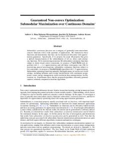
Fig. 1. (Left) The initial formation pose for a set of 100 nodes in (center, right) The final formation trajectory/pose that achieves the desired shape while minimizing the total distance that the team must travel. The optimal values were 107.612 for scale, −22.403 degrees for orientation and (9.059, 71.72)T for translation.
These 2(m − 2) constraints are now convex (in fact, linear) functions of our state vector q = (q1 , . . . , qm )T . They are also necessary and sufficient for describing the formation shape [19]. Writing these constraints in matrix form Aq = 0, we see a further advantage is that they implicitly define a low-dimensional representation for the formation, as the dimension of the nullspace dim(N (A)) = 4. The four free variables correspond to the translation, rotation, and scale of the shape as defined in (5). The problem of finding the formation pose Q can now be posed as either of the following constrained optimization problems m P min max k qi − pi k2 min k qi − pi k2 q i=1,...,m q i=1 (9) s.t. Aq = 0 s.t. Aq = 0 where the former corresponds to our minimax distance metric defined in Problem 3.2.1 and the latter our total distance metric. While both the constraints and objective functions of these problems are convex, the form of the latter does not lend itself to traditional optimization techniques. To remedy this, we augment the state vector q with an auxiliary variable t1 for our minimax metric, and with m auxiliary variables t = (t1 , . . . , tm )T for our total distance metric. The problems in (9) can thus be restated min t1
min 1Tm t
s.t. yi ≤ t1 , i = 1, . . . , m Aq = 0
s.t. yi ≤ ti , i = 1, . . . , m Aq = 0
q,t
q,t1
(10) where yi , k qi − pi k2 . Both forms are equivalent. However, the objectives in (10) are now twice differentiable. We have also introduced m convex second-order conic constraints. These problems are now secondorder cone programs, and they can be solved efficiently using modern interior point algorithms [22]. A. Regulating Shape Parameters Through the use of additional linear and second-order cone constraints, we can regulate the rotation, translation, and scale of the formation shape. Constraining the minimum and maximum orientation (θmin , θmax ) can be accomplished through a pair of linear constraints (q2 − q1 )T (− sin θmax , cos θmax ) ≤ 0 (q2 − q1 )T (sin θmin , cos θmin ) ≤ 0
(11)
Constraining the translation and the maximum scale of the formation can be respectively done using second-order cone constraints k q1 − p1 k2 ≤ tmax ,
k q2 − q1 k2 ≤ αmax
(12)
Note, however, that constraints of the form k q2 − q1 k2 ≥ αmin ,
k q2 − q1 k2 = α
(13)
are not convex. If regulating the minimum scale is required, we have developed an efficient approximation method based upon our results for fixed orientations in R2 and R3 . The interested reader is referred to [27] for further details. B. Simulation Results Figure 1 shows a simulation trial demonstrating the process. In this example, 100 nodes were tasked with transitioning to a new shape while minimizing the total distance traveled. While deliberately contrived, this example demonstrates the efficacy of our approach. The formation is able to optimally transition from an arbitrary shape to a very specific shape. This would typically be the case when a formation of robots was initially deployed. In this example, none of the shape parameters (i.e., translation, rotation, or scale) were regulated. V. O N C OMPLEXITY To be suitable for use in large-scale formations, the shape problem needs to feature low computational complexity as well as be solvable in real-time. In this section, we show that it can be solved in only O(m1.5 ) basic operations. To this end, we employ a simple logarithmic barrier approach [5]. For the sake of brevity, the results presented here are specific to the minimax distance problem. However, we have obtained similar results for the total distance problem variation as well [12]. This includes both the regulated and unregulated shape problem formulations. A. Reformulating the Shape Problem The original minimax shape planning problem can be restated in a relaxed form suitable for solving via the barrier approach. Conversion requires augmenting the objective function given in (10) with log-barrier terms corresponding to the problem’s conic constraints as follows: m P log (t21 − (qi − pi )T (qi − pi )) min τk t1 − q,t1 (14) i=1 s. t. Aq = 0 where τk is the inverse log-barrier scaler for the kth iteration. Essentially, solving our SOCPs reduces to solving a sequence of convex optimization problems of this form, where after each iteration τk+1 is chosen such that τk+1 = µk τk with µ ∈ R, µ > 1 being an algorithmic constant. B. Banding the Newton KKT System During each iteration of the log-barrier approach, we aim to minimize the second-order Taylor approximation of our objective as a function of the Newton step, δx, subject to Aδx = 0. As a result, obtaining δx is equivalent to analytically solving the Karush-Kuhn-Tucker (KKT) conditions associated with this
0
0
0
50
50
100
100
150
150
200
200
250
250
10
20
30
40
50
60
70
80 300
90
0
10
20
30
40
50 nz = 661
60
70
80
90
300
0
50
100
150 200 nz = 1149
250
300
0
50
100
150 200 nz = 1149
250
300
Fig. 2. (Left) The nominal Newton KKT system sparsity structure for the minimax motion planning problem in SE(2). (Center) Augmented Newton KKT system sparsity structure. (Right) The banded system with lower and upper bandwidths of 8. This system is now solvable in O(m) time.
equality-constrained sub-problem [5]. In other words, we must solve the following linear system of equations [5]: „ « « „ «„ H AT −g δx (15) = 0 w A 0 where H and g respectively denote the evaluated Hessian and gradient of the objective function given in (14) at x, w is the corresponding dual variable for δx, and A is as previously defined. Solving (15) is the bottleneck of the algorithm. However, we will show that it can be solved in linear time by reposing (14). Noting that the coefficient matrix of (15) is symmetric indefinite, we employ Gaussian elimination with non-symmetric partial pivoting. The performance of this technique suffers significantly when the linear system in question features dense rows and/or columns due to fill-in [26]. In particular, the algorithm would yield a worst-case performance of O(m3 ) when solving (15) for the problem formulation given in (14). Such a workload is highly impractical when considering large-scale configurations that feature 1000’s of decision variables. To address this issue, we instead employ an auxiliary formulation of (14) that facilitates transforming the Newton KKT system into a mono-banded form min q,t
s. t.
τk m
m P
i=1
ti −
s2 k2 (qlx s2 k2 (qly
m P
i=1
log (t2i − (qi − pi )T (qi − pi ))
dxj ) dyj )
(sxl , −syl )T (dj+1 − dj ) (syl , sxl )T (dj+1 − dj )
k − = k − = ti+1 = ti , i = 1, . . . , m − 1 d2i+1 = d2i−1 , i = 1, . . . , m − 3 d2(i+1) = d2i , i = 1, . . . , m − 3 di = qi , i ∈ {1, 2}
(16)
where the first equality holds due to the constraints placed on ti . 1) Banding the Linear System: Given this augmented formulation, our claim is that the system can be made mono-banded. To show this, we begin by defining the initial solution vector ordering for (15) as it corresponds to problem (16) as follows: “ ”T δη1T , δη2T , δκT1 , . . . , δκT(m−2) , µT (18) δηi =
δqi δti
«
1 0 1 w1 δd2(i−1)+1 C B .. δκi = @ δd2(i−1)+2 A µ = @ A . δη(i+2) w7m−13 0
̺1 , q1x = dx1 ̺2 , q1y = dy1 ̺ 3 , t1 = t2
̺4 , q2x = dx2 ̺5 , q2y = dy2
(19)
Similarly, for 3 ≤ i ≤ (m − 1), we define the constraints associated with qi as: ϕi1 ϕi2 ϕi3 ϕi4 ϕi5 ϕi6 ϕi7
, , , , , , ,
k s2 k2 (qix − dxj ) = (sxi , −syi )T (dj+1 − dj ) k s2 k2 (qiy − dyj ) = (syi , sxi )T (dj+1 − dj ) ti = ti−1 dxj+2 = dxj dyj+2 = dyj dxj+3 = dxj+1 dyj+3 = dyj+1
(20)
where j is as previously defined. With qm , we associate the remaining three constraints:
for l = 3, . . . , m and where j = 2(i − 3) + 1. Notice that the objective has changed; however, we see that both forms are equivalent since: m m “τ ” τk X τk X k mt1 = τk t1 (17) ti = t1 = m i=1 m i=1 m
„
where the δ variables correspond to the primal Newton step components associated with each of the system variables, and wj denotes the dual variable associated with the j th constraint. In order to yield the mono-banded form, we begin by stating the constraint/row permutation for A that yields the tri-banded system appearing Figure 2 (Center). We assume that A is already arbitrarily constructed with random row and column permutations. For the sake of clarity, we group constraints by associating them with the respective nodes that introduce them into the system. In doing so, we employ a slight abuse of notation by allowing qi to also denote the ith robot in the configuration. That stated, we now define the constraints associated with q1 and q2 as:
x k s2 k2 (qm − dxj ) = (sxm , −sym )T (dj+1 − dj ) y k s2 k2 (qm − dyj ) = (sym , sxm )T (dj+1 − dj ) tm = tm−1 (21) where j is as previously stated with i = m. Again employing a slight abuse of notation, we let each ϕij denote the initial row index of its associated constraint. As such, we provide the following row permutation for A. This ordering yields the tri-banded form appearing in Figure 2 (Center): “ ”T T ϑT , κ1T , . . . , κ(m−1) , ςT (22)
ϕm1 ϕm2 ϕm3
, , ,
0
B B ϑ=B @
̺1 ̺2 .. . ̺5
0 ϕ(i+2)1 C B ϕ(i+2)2 C B C κi = B .. A @ . ϕ(i+2)7 1
1
0 1 ϕm1 C C C ς = @ ϕm2 A A ϕm3
Given this definition of A as well as (18), the mono-banded form of (15) can be constructed. Symmetrically applying the
permutation that yields the following solution vector ordering: “ ”T T λT , ξ1T , . . . , ξ(m−3) , χT (23) 1 0 0 1 1 0 δd2(i−1)+1 δd2m−5 δη1 B δd2(i−1)+2 C B δd2m−4 C C B B w1 C B C C B w6+7(i−1) C B B w7m−15 C C B B . C B C χ = λ = B .. C ξi = B C .. B w7m−14 C C C B B B C . C B @ w5 A @ w7m−13 A @ w12+7(i−1) A δη2 δηm δη(i+2) produces a mono-banded coefficient structure having a total bandwidth of 17. Figure 2 illustrates this process of transforming the Newton KKT system. The “augmented” system derived from the permutations given in (18) and (22) is shown in Figure 2 (Center). Taking the coefficient structure of (15) in this form and symmetrically permuting its rows and columns according to (23) yields the mono-banded system appearing in Figure 2 (Right). It can now be solved in O(m) using a band-diagonal LU -based solver [25].
where δt denotes the time-step, and vimax denotes the velocity limits of the ith robot. This would allow less mobile or even fixed (anchor) nodes to be accommodated. Others might be expressed as linear constraints. As an example, a formation wanting to maintain positive velocity in the y-direction could ensure this by specifying a minimum forward distance traveled dmin for each node as qiy − pyi ≥ vimin δt, i ∈ {1, . . . , m}
(25)
In summary, if the constraints can be expressed in terms of some combination of feasible linear, second-order cone, or semidefinite constraints, they can be directly integrated into our framework. Furthermore, as with the environmental constraints discussed in Section VII, the motion constraints introduced by the ith node are only a function of its own initial and final positions. As a result, the mono-banded structure and complexity results derived in Section V will again be preserved.
C. Complexity in Practice
√ Modern interior-point methods (IPMs) require m iterations to converge [22]. However, it is well-known that this computational bound is extremely conservative and that iteration complexity in practice is O(1) [5]. Consequently, solving the shape problems requires only O(m) basic operations in practice.
(a)
(b)
Fig. 4. Shape transitions for two teams of 15 robots, each respectively aligned along an in-line path. In this case, the teams were charged with obtaining a triangular formation while minimizing the minimax distance metric. (a-Left) With no motion constraints. (a-Right) With qiy − pyi ≥ 0, i = 1, . . . , m. (b) The final configurations obtained by the respective teams. Including the motion constraints increased the minimax distance for the formation by 87% in this case.
Fig. 3. The mean CPU time required to solve the unregulated total distance metric shape problem using the Mosek industrial solver. Each point corresponds to the mean for a sample of 100 randomly generated shape SOCPs. The trend is strongly linear with r 2 = 0.9905.
Simulation Results: A total of 20,000 instances of the unregulated total distance problem were solved using the Mosek industrial package [24]. Values of m were considered between 10 and 2000 using a step size of 10. For each configuration size, a total of 100 random problem instances were solved. All problems were solved on standard desktop PC having a 3.0 GHz Pentium 4 processor. From Figure 3, we see the time complexity scales as O(m) with r 2 = 0.9905, where r is the correlation coefficient. Furthermore, the data indicates that for a team of up to 2000 robots, the problem can be solved in less than 300 milliseconds! VI. I NTEGRATING M OTION C ONSTRAINTS This framework relies upon the convexity of the underlying problem to efficiently solve coordination problems for large formations. As a consequence, motion constraints can also be accommodated so long as they can be expressed similarly. For example, to this point we have generated objective node positions without consideration for vehicle constraints. However, we could readily accommodate velocity constraints as second-order cone constraints of the form k qi − pi k2 ≤ vimax δt
(24)
Simulation Results: A sample simulation showing the same formation shape change with (triangles) and without (circles) motion constraints is presented in Figure 4. In both cases, the objective was for the teams to transition from an initial in-line path configuration to a triangular shaped formation. Optimization was over our minimax metric. In the former, the minimum forward distance traveled for each node was constrained as qiy − pyi ≥ 0, i ∈ {1, . . . , m}. Scale and orientation were fixed in both cases. In this case, the additional constraints increased the minimax distance for shape formation by 87%. VII. I NTEGRATING W ORKSPACE C ONSTRAINTS A straightforward extension to regulating the formation shape would be to ensure the final configuration resides within the bounds of the operational environment. If we assume that the workspace C can be modeled via k linear inequalities yielding a convex space, e.g. C = {x ∈ R2 : Ac x ≤ bc }
(26)
this will introduce km additional constraints where m again denotes the number of agents in the configuration. However, the core linear system will remain mono-banded, as the k constraints introduced for the ith team member’s position are only a function of the node’s position in the final formation (i.e. qi ). Moreover, the coefficients of these constraints can be chained locally by introducing 2k auxiliary variables for each robot [11]. As a consequence, the linear system is solvable in O(km) time, and the corresponding SOCP can be solved in O(km) time in practice – or linear time in the size of the formation and the environment.
25
0
20
1000
15
2000
10
3000
5
4000
0
5000
−5
6000
−10
7000
−15
8000
−20 −40
9000
−30
−20
−10
0
10
20
30
40
0
1000
2000
3000
4000 5000 nz = 20559
6000
7000
8000
9000
Fig. 5. (Left) Two problem instances with (stars) and without (circles) boundary constraints. In this example, the workspace limits constrained the scale of the optimal solution from α = 85 to α = 59.85. (Right) The mono-banded form of the problem instance with workspace constraints.
Simulation Results: In this example, we considered a variation of the shape problem where the objective function was modified to maximize the scale of the formation subject to workspace boundary constraints. Such a result might prove useful for tasks such as maximizing sensor network coverage while satisfying a desired shape geometry. In this example, the orientation of the shape was fixed. Figure 5 illustrates the results obtained for a team of 101 nodes in SE(2). Both constrained and unconstrained problem solutions are presented to illustrate the influence of the convex workspace model. The non-zero dot plot of the Newton KKT system is also shown to highlight that the mono-banded structure of the linear system remains intact. VIII. M OTION P LANNING IN P OLYGONAL E NVIRONMENTS Extending the results of Section VII, we now consider motion planning in a polygonal environment with obstacles. Obstacles highlight a significant limitation of convexification approaches. Recall the underlying assumption of (26) was that the workspace could be defined through a finite number of convex constraints. When we introduce obstacles into the workspace, we create voids in the feasible set. The result is a loss of convexity, and the corresponding optimization problem becomes significantly more difficult to solve. While convex relaxations present one potential remedy [9], we instead take inspiration from [2] and employ a hierarchical discrete-continuous optimization approach. We assume the configuration space for the robot team C is a polygonal environment with obstacle subspace O and free space Cf ree such that Cf ree = C − O. Using exact cell decomposition methods (e.g. triangulation, trapezoidal decomposition, etc.), Cf ree can be tessellated into convex polygonal cells C1 , . . . , Cz , S where Cf ree = zi=1 Ci [6]. The resulting partition induces an undirected graph G = (V, E), where vertex vi ∈ V corresponds to cell Ci , and edge eij ∈ E implies that there exists a common edge between Ci and Cj . Paths between cells can then be efficiently computed using traditional graph optimization algorithms (e.g. [13]). The motion planning problem can then be reposed as transitioning the formation from cell to cell along the specified path. In the sequel, we assume a triangulation partition of Cf reeS . We further assume that the union of adjacent cells Cij = Ci Cj ∀ (Ci , Cj ) ∈ E is convex. While this may appear restrictive, it is straightforward to refine any pair of adjacent triangles to three such triangles where both of the resulting adjacent pairs meet this constraint. RemarkS8.1: Given two adjacent cells (Ci , Cj ) ∈ E, where Cij = Ci Cj is convex, if node xi ∈ Ci and xj ∈ Cj , then by convexity λxi +(1−λ)xj ∈ Cij , λ ∈ [0, 1]. This implies that for a formation of m nodes with initial pose Xi = (xi1 , . . . , xim )T ∈ R2m in triangle Ci , and final pose Xj in triangle Cj , the paths of each node will remain entirely in Cij ⊆ Cf ree . This guarantees
against collisions with obstacles. Let us assume that such a path Cp = {C1 , . . . , Ck } ⊆ Cf ree has been specified by a higher level planner. Our motion planning problem can then be written as follows: Problem 8.2: Given a path specification Cp = {C1 , . . . , Ck }, a corresponding shape specification S = {S1 , . . . , Sk }, and an initial formation pose X0 , find a motion sequence X = {X1 , . . . , Xk } for the formation such that 1) Xi ∼ Si , i = 1, . . . , k 2) Xi ∈ Ci , i = 1, . . . , k 3) The distance traveled by the formation is minimized in accordance with the criteria from Problem 3.2. In solving Problem 8.2, we employ optimization techniques from model predictive control [18], [23]. In this context, however, the length of the horizon is not defined by time, but rather the length of the path over which the optimization problem is solved. To constrain the pose of the formation during each step of the horizon, each triangle can be modeled as a set of three linear inequality constraints on the position of each node: cTil xij ≤ 0, i = 1 . . . k, j = 1 . . . m, l = 1 . . . 3
(27)
In a slight abuse of notation, we also let Ci = (c11 , . . . , cm3 )T ∈ R3m× 2m denote the set of linear constraints on the formation pose such that Xi ∈ Ci . We can now write the solution to Problem 8.2 for our total distance metric as: k P m P tij , i = 1 . . . k, j = 1 . . . m min X
s.t.
i=1 j=1
k xij − xi−1,j k2 ≤ tij Ai Xi = 0 Ci Xi ≤ 0
(28)
where Ai are the constraints associated with shape Si as defined in Section IV. This problem is also a SOCP. More significantly perhaps, the corresponding Newton KKT matrix corresponds to the chaining of k instances of our single step problem. As a result, the associated linear system will remain mono-banded; however, in this case the bandwidth will grow as either a function of m or k depending upon the selected permutation of the augmented KKT system. As such, we conclude the theoretical complexity is O(k1.5 m3.5 ) or O(k3.5 m1.5 ) – once again depending upon the chosen ordering. Simulation Results: A sample simulation trial for a formation of 16 robots is shown at Figure 6. The path of the formation is specified by a higher level planner after a discrete optimization phase on the corresponding graph G (Left). The formation then solves the continuous optimization problem specified in (28). The resulting path of the formation is shown in Figure 6 (Center). In this example, the optimization was over the entire path length (k = 15), the shape was held constant, and the minimum scale of the formation was specified (as a premise for collision avoidance). IX. D ISCUSSION The thrust of this work was to highlight the potential for employing convex optimization techniques to coordinate the motion of large-scale robot formations. Recent advances in the underlying algorithms allow large-scale motion planning problems to be solved online, and with a complexity that in practice scales linearly in the size of the formation and/or the environment. Key to our results was a formal definition of shape for describing the formation pose. This provides an implicitly low-dimensional representation that can be defined via linear equality constraints. Optimal shape changes can then be solved as SOCPs.
0
500
1000
1500
2000
2500
3000
3500
4000
0
500
1000
1500
2000 2500 nz = 15378
3000
3500
4000
Fig. 6. (Left) Cpath as specified by the higher level planner. (Center) The corresponding motion sequence obtained from solving the associated SOCP. The formation is guaranteed to follow Cpath while minimizing the total distance traveled, avoiding obstacles, and maintaining the desired formation shape. In this example, the orientation and minimum scale for the formation were constrained. (Right) The linear system remains mono-banded.
Worth noting is that our framework also lends itself to a distributed implementation that affords expected per-node computational, message, and storage complexities of O(1) [10]. It can be adapted for use with any IPM that preserves the separability of the objective with respect to each team member. The convexity requirement has its limitations, such as when considering non-holonomic kinematic motion models. However, the optimal paths generated for the fully actuated robots can still be followed by differential drive/tracked vehicles, which see widespread use in mobile robotics. Although the results will no longer be optimal for such robots, they should still be quite good in practice. We should also point out that while the work presented in this paper focused on operations in the plane, we have similar results in R3 for fixed orientations [27]. Extending these results to operations in SE(3) is currently a topic of ongoing research. Other extensions to this work are also possible. One of our current interests is formation/network coverage and using robust estimation techniques to relax the shape constraints for improving system performance. We are also exploring ways to generalize our problem so as to provide optimal node assignments while yielding an optimal shape formation pose. Finally, the problem of finding optimal shape changes relates to the point pattern matching problem [28], and we are looking to apply our results to this as well as point-wise deformations in computer graphics. X. ACKNOWLEDGMENTS Special thanks to Ali Jadbabaie for discussions on IPM complexity, and Rafael Fierro on the coordination of robot formations. R EFERENCES [1] R. Bachmayer and N. E. Leonard. Vehicle networks for gradient descent in a sampled environment. In Proc. IEEE Conf. on Decision and Control, Las Vegas, NV, Dec 2002. [2] C. Belta, V. Isler, and G. Pappas. Discrete abstractions for robot motion planning and control in polygonal environments. TRO, 21(5):864–874, Oct 2005. [3] C. Belta and V. Kumar. Abstraction and control for groups of robots. IEEE Trans. on Robotics and Automation, 2004. [4] C. Belta and V. Kumar. Optimal motion generation for groups of robots: a geometric approach. ASME Journal of Mechanical Design, 126, 2004. [5] S. Boyd and L. Vandenberghe. Convex Optimization. Cambridge Unviersity Press, 2004. [6] H. Choset, K. Lynch, S. Hutchinson, G. Kantor, W. Burgard, L. Kavraki, and S. Thrun. Principles of Robot Motion Planning. MIT Press, 2005. [7] J. Cort´es, S. Mart´ınez, T. Karatas, and F. Bullo. Coverage control for mobile sensing networks. IEEE Trans. on Robotics and Automation, 20(2):243–255, April 2004. [8] A. K. Das, R. Fierro, V. Kumar, J. P. Ostrowski, J. Spletzer, and C. J. Taylor. A vision-based formation control framework. IEEE Trans. on Robotics and Automation, 18(5):813–825, October 2002.
[9] A. d’Aspremont and S. Boyd. Relaxations and randomized methods for nonconvex QCQPs. Stanford University, 2003. [10] J. Derenick, C. Mansley, and J.Spletzer. Efficient motion planning strategies for large-scale sensor networks. In Proceedings of the Seventh International Workshop on the Algorithmic Foundations of Robotics (WAFR 2006), New York, NY, USA, July 2006. [11] J. Derenick and J. Spletzer. to appear in Advances in Cooperative Control and Optimization, chapter Second-order Cone Programming (SOCP) Techniques for Coordinating Large-scale Robot Teams in Polygonal Environments. Springer. [12] J. Derenick and J. Spletzer. TR LU-CSE-05-029: Optimal shape changes for robot teams. Technical report, Lehigh University, 2005. [13] E. Dijkstra. A note on two problems in connexion with graphs. Numerische Mathematik, 1:269–272, 1959. [14] I. L. Dryden and K. V. Mardia. Statistical Shape Analysis. John Wiley and Sons, 1998. [15] J. T. Feddema, R. D. Robinett, and R. H. Byrne. An optimization approach to distributed controls of multiple robot vehicles. In Workshop on Control and Cooperation of Intelligent Miniature Robots, IEEE/RSJ IROS, Las Vegas, Nevada, October 31 2003. [16] N. Heo and P. K. Varshney. Energy-efficient deployment of intelligent mobile sensor networks. Systems, Man and Cybernetics, Part A, IEEE Transactions on, 35(1):78–92, 2005. [17] A. Howard, M. J. Mataric, and G. S. Sukhatme. An incremental self-deployment algorithm for mobile sensor networks. Autonomous Robots, 13(2):113–126, September 2002. [18] A. Jadbabaie, J. Yu, and J. Hauser. Unconstrained receding-horizon control of nonlinear systems. IEEE Trans. on Automatic Control, 46(5):776–783, May 2001. [19] D. Kendall, D. Barden, T. Carne, and H. Le. Shape and Shape Theory. John Wiley and Sons, 1999. [20] H. W. Kuhn. The Hungarian method for the assignment problem. Naval Research Logistics Quarterly 2, pages 83–97, 1955. [21] S. LaValle and S. Hutchinson. Optimal motion planning for multiple robots having independent goals. IEEE Trans. on Robotics and Automation, 14(6):912–925, Dec. 1998. [22] M. Lobo, L. Vandenberghe, S. Boyd, and H. Lebret. Applications of second-order cone programming. Linear Algebra and Applications, Special Issue on Linear Algebra in Control, Signals and Image Processing, 1998. [23] D. Mayne, J. Rawings, C. Rao, and P. Scokaert. Constrained model predictive control: Stability and optimality. Automatics, 36(6):789– 814, June 2000. [24] MOSEK ApS. The MOSEK Optimization Tools Version 3.2 (Revision 8) User’s Manual and Reference. http://www.mosek.com. [25] W. Press et al. Numerical Recipes in C. Cambridge University Press, 1993. [26] Y. Saad. Iterative Methods for Sparse Linear Systems. Society for Industrial and Applied Mathematics, Philadelphia, PA, USA, 2003. [27] J. Spletzer and R. Fierro. Optimal positioning strategies for shape changes in robot teams. In Proc. IEEE Int. Conf. Robot. Automat., 2005. [28] P. B. V. Wamelen, Z. Li, and S. S. Iyengar. A fast algorithm for the point pattern matching problem. Pattern Recognition, 37(8):1699– 1711, August 2004. [29] F. Zhang, M. Goldgeier, and P. S. Krishnaprasad. Control of small formations using shape coordinates. In Proc. IEEE Int. Conf. Robot. Automat., volume 2, Taipei, Sep 2003.