Contributions to Batch Mode Reinforcement Learning
PhD dissertation by Raphael Fonteneau
Department of Electrical Engineering and Computer Science, University of Li`ege, BELGIUM 2011
ii
Foreword When I was studying electrical engineering and computer science at the French Grande Ecole SUPELEC (Ecole Sup´erieure d’Electricit´e), I had the opportunity to work with Dr. Damien Ernst, who was professor there, on a research project dealing with the use of system theory for better understanding the dynamics of the HIV infection. This first experience was the trigger to pursue this research adventure at the University of Li`ege (Belgium) under the supervision of Dr. Damien Ernst and Prof. Louis Wehenkel on the practical problem of extracting decision rules from clinical data in order to better treat patients suffering from chronic-like diseases. This problem is often formalized as a batch mode reinforcement learning problem. The work done during my PhD thesis enriches this body of work in batch mode reinforcement learning so as to try to bring it to a level of maturity closer to the one required for finding decision rules from clinical data. Most of the research exposed in this dissertation has been done in collaboration with Prof. Susan A. Murphy from the University of Michigan who has pioneered the use of reinforcement learning techniques for inferring dynamic treatment regimes, and who has had the kindness to invite me in her lab in November 2008. This dissertation is a collection a several research publications that have emerged from this work.
iii
iv
Acknowledgements First and foremost, I would like to express my deepest gratitude and appreciation to Dr. Damien Ernst, for offering me the opportunity to discover the world of research. All along these four years, he proved to be a great collaborator on many scientific and human aspects. The present work is mostly due to his support, patience, enthusiasm, creativity and, of course, personal friendship. I would like to extend my deepest thanks to Prof. Louis Wehenkel for his up to the point suggestions and advice regarding every research contribution reported in this dissertation. His remarkable talent and research experience have been very valuable at every stage of this research. My deepest gratitude also goes to Prof. Susan A. Murphy for being such an inspiration in research, for her suggestions and for her enthusiasm. I would also like to thank her very much for welcoming me in her lab at the University of Michigan. I also address my warmest thanks to all the SYSTMOD research unit, the Department of Electrical Engineering and Computer Science, the GIGA and the University of Li`ege, where I found a friendly and stimulating research environment. Many thanks to the academic staff, especially to Dr. Pierre Geurts, Prof. Quentin Louveaux and Prof. Rodolphe Sepulchre. A special acknowledgement to my office neighbors, Bertrand Corn´elusse and Renaud Detry. Many additional thanks to Julien Becker, Vincent Botta, Anne Collard, Boris Defourny, Guillaume Drion, Fabien Heuze, Samuel Hiard, Vˆan-Anh Huynh-Thu, Michel Journ´ee, Thibaut Libert, David Lupien St-Pierre, Francis Maes, Alexandre Mauroy, Gilles Meyer, Laurent Poirrier, Pierre Sacr´e, Firas Safadi, Alain Sarlette, Franc¸ois Schnitzler, Olivier Stern, Laura Trotta, Wang Da and many other colleagues and friends from Montefiore and the GIGA that I forgot to mention here. I also would like to thank the administrative staff of the University of Li`ege, and, in particular, Marie-Berthe Lecomte, Charline Ledent-De Baets and Diane Zander for their help. I also would like to thank all the scientists, non-affiliated with the University of Li`ege, with whom I have had interesting scientific discussions, among others: Lucian v
Busoniu, Bibhas Chakraborty, Jing Dai, Matthieu Geist, Wassim Jouini, Eric Laber, Daniel Lizotte, Marie-Jos´e Mhawej, Mahdi Milani Fard, Claude Moog, Min Qian, Emmanuel Rachelson, Guy-Bart Stan and Peng Zhang. Many thanks to the members of the jury for carefully reading this dissertation and for their advice to improve its quality. I am very grateful to the FRIA (Fonds pour la Formation a` la Recherche dans l’Industrie et dans l’Agriculture) from the Belgium fund for scientific research FRSFNRS and to the PAI (Poles d’Attraction Interuniversitaires) BIOMAGNET (Bioinformatics and Modeling: from Genomes to Networks) and DYSCO (Dynamical Systems, Control and Optimization).
Finally, I would like to express my deepest personal gratitude to my parents for teaching me the value of knowledge and work, and of course, for their love. Many thanks to my sisters Adeline and Anne-Elise, my brother Emmanuel, my whole family and family-in-law, and longtime friends for their unconditional support before and during these last four years.
Thank you to my little Gabrielle for her encouraging smiles.
To you Florence, my beloved wife, no words can express how grateful I feel. Thank you for everything.
Raphael Fonteneau Li`ege, January 2011.
vi
Abstract This dissertation presents various research contributions published during these four years of PhD in the field of batch mode reinforcement learning, which studies optimal control problems for which the only information available on the system dynamics and the reward function is gathered in a set of trajectories. We first focus on deterministic problems in continuous spaces. In such a context, and under some assumptions related to the smoothness of the environment, we propose a new approach for inferring bounds on the performance of control policies. We also derive from these bounds a new inference algorithm for generalizing the information contained in the batch collection of trajectories in a cautious manner. This inference algorithm as itself lead us to propose a min max generalization framework. When working on batch mode reinforcement learning problems, one has also often to consider the problem of generating informative trajectories. This dissertation proposes two different approaches for addressing this problem. The first approach uses the bounds mentioned above to generate data tightening these bounds. The second approach proposes to generate data that are predicted to generate a change in the inferred optimal control policy. While the above mentioned contributions consider a deterministic framework, we also report on two research contributions which consider a stochastic setting. The first one addresses the problem of evaluating the expected return of control policies in the presence of disturbances. The second one proposes a technique for selecting relevant variables in a batch mode reinforcement learning context, in order to compute simplified control policies that are based on smaller sets of state variables.
vii
viii
R´esum´e Ce manuscrit rassemble diff´erentes publications scientifiques r´ealis´ees au cours de ces quatre ann´ees de th`ese dans le domaine de l’apprentissage par renforcement en mode “batch”, dans lequel on souhaite contrˆoler de mani`ere optimale un syst`eme pour lequel on ne connait qu’un ensemble fini de trajectoires donn´ees a priori. Dans un premier temps, cette probl´ematique a e´ t´e d´evelopp´ee dans un contexte d´eterministe, en consid´erant des espaces continus. En travaillant sous certaines hypoth`eses de r´egularit´e de l’environnement, une nouvelle approche de calcul de bornes sur les performances des lois de contrˆole a e´ t´e developp´ee. Cette approche a ensuite permis le d´evelopement d’un algorithme d’inf´erence de loi de contrˆole abordant le probl`eme de g´en´eralisation de mani`ere pr´ecautionneuse. De mani`ere plus formelle, une r´eflexion sur la possibilit´e de g´en´eraliser suivant le paradigme min max a e´ galement e´ t´e propos´ee. Lorsque l’on travaille en mode batch, on doit e´ galement souvent faire face au probl`eme relatif a` la g´en´eration de bases de donn´ees aussi informatives que possible. Ce probl`eme est abord´e de deux mani`eres diff´erentes dans ce manuscrit. La premi`ere consiste a` faire appel aux bornes d´ecrites ci-dessus dans le but de g´en´erer des donn´ees menant a` une augmentation de la pr´ecision de ces bornes. La deuxi`eme propose de g´en´erer des donn´ees en des endroits pour lesquels il est pr´edit (en utilisant un mod`ele de pr´ediction) qu’une modification de la loi de contrˆole courante sera induite. La majorit´e des contributions rassembl´ees dans ce manuscrit consid`erent un environnement d´eterministe, mais on y pr´esente e´ galement deux contributions se plac¸ant dans un environnement stochastique. La premi`ere traite de l’´evaluation de l’esp´erance du retour des lois de contrˆole sous incertitudes. La deuxi`eme propose une technique de s´election de variables qui permet de construire des lois de contrˆoles simplif´ees bas´ees sur des petits sous-ensembles de variables.
ix
x
Contents Foreword
iii
Acknowledgements
v
Abstract
vii
R´esum´e
ix
1
1 2 3 3
Overview 1.1 Introduction . . . . . . . . . . . . . . . . . . . . . . . . . . . 1.1.1 Batch mode reinforcement learning . . . . . . . . . . 1.1.2 Main contributions presented in this dissertation . . . 1.2 Chapter 2: Inferring bounds on the performance of a control from a sample of trajectories . . . . . . . . . . . . . . . . . . 1.3 Chapter 3: Towards min max generalization in reinforcement learning . . . . . . . . . . . . . . . . . . . . 1.4 Chapter 4: Generating informative trajectories by using bounds on the return of control policies . . . . . . . . 1.5 Chapter 5: Active exploration by searching for experiments that falsify the computed control policy . . . . . . . . . . . . . . . . . . . . . . . . . . 1.6 Chapter 6: Model-free Monte Carlo–like policy evaluation . . . . . . . . . . . . . . . . . . . . . . . . 1.7 Chapter 7: Variable selection for dynamic treatment regimes: a reinforcement learning approach . . . . . . . . . . . . . . . . . . . . . . . . . . . . . 1.8 List of publications . . . . . . . . . . . . . . . . . . . . . . . xi
. . . . . . . . . . . . policy . . . .
4
. . . .
6
. . . .
7
. . . .
8
. . . .
10
. . . . . . . .
12 14
2
3
4
5
Inferring bounds on the performance of a control policy from a sample of trajectories 2.1 Introduction . . . . . . . . . . . . . . . . . . . . . . . . . . . . . . . 2.2 Formulation of the problem . . . . . . . . . . . . . . . . . . . . . . . 2.3 Lipschitz continuity of the state-action value function . . . . . . . . . 2.4 Computing a lower bound on J h (x0 ) from a sequence of four-tuples . . . . . . . . . . . . . . . . . . . . . . . . . 2.5 Finding the highest lower bound . . . . . . . . . . . . . . . . . . . . 2.6 Tightness of the lower bound LhFn (x0 ) . . . . . . . . . . . . . . . . . 2.7 Conclusions and future research . . . . . . . . . . . . . . . . . . . . Towards min max generalization in reinforcement learning 3.1 Introduction . . . . . . . . . . . . . . . . . . . . . . . . . . . . . . . 3.2 Related work . . . . . . . . . . . . . . . . . . . . . . . . . . . . . . 3.3 Problem Statement . . . . . . . . . . . . . . . . . . . . . . . . . . . 3.4 Reformulation of the min max problem . . . . . . . . . . . . . . . . 3.5 Lower bound on the return of a given sequence of actions . . . . . . . 3.5.1 Computing a bound from a given sequence of one-step transitions 3.5.2 Tightness of highest lower bound over all compatible sequences of one-step transitions . . . . . . . . . . . . . . . . . . . . . 3.6 Computing a sequence of actions maximizing the highest lower bound 3.6.1 Convergence of (˜ u∗Fn ,0 (x0 ), . . . , u ˜∗Fn ,T −1 (x0 )) towards an optimal sequence of actions . . . . . . . . . . . . . . . . . . . . 3.6.2 Cautious Generalization Reinforcement Learning algorithm . 3.7 Illustration . . . . . . . . . . . . . . . . . . . . . . . . . . . . . . . . 3.8 Discussion . . . . . . . . . . . . . . . . . . . . . . . . . . . . . . . . 3.9 Conclusions . . . . . . . . . . . . . . . . . . . . . . . . . . . . . . .
21 22 24 26 29 33 34 38 43 45 46 47 50 54 56 61 64 65 68 69 74 75
Generating informative trajectories by using bounds on the return of control policies 4.1 Introduction . . . . . . . . . . . . . . . . . . . . . . . . . . . . . . . 4.2 Problem statement . . . . . . . . . . . . . . . . . . . . . . . . . . . 4.3 Algorithm . . . . . . . . . . . . . . . . . . . . . . . . . . . . . . . .
81 82 82 83
Active exploration by searching for experiments that falsify the computed control policy 5.1 Introduction . . . . . . . . . . . . . . . . . . . . . . . . . . . . . . . 5.2 Problem statement . . . . . . . . . . . . . . . . . . . . . . . . . . . 5.3 Iterative sampling strategy to collect informative system transitions . .
89 90 91 92
xii
5.4
5.5
5.6 5.7 6
7
5.3.1 Influence of the BM RL algorithm and the predictive model P M 94 5.3.2 Influence of the Ln sequence of parameters . . . . . . . . . . 95 BM RL/P M implementation based on nearest-neighbor approximations . . . . . . . . . . . . . . . . . . . . 95 5.4.1 Choice of the inference algorithm BM RL . . . . . . . . . . 95 Model learning–type RL . . . . . . . . . . . . . . . . . . . . 95 Voronoi tessellation-based RL algorithm . . . . . . . . . . . . 96 5.4.2 Choice of the predictive model P M . . . . . . . . . . . . . . 98 Experimental simulation results with the car-on-the-hill problem . . . 100 5.5.1 The car-on-the-hill benchmark . . . . . . . . . . . . . . . . . 100 5.5.2 Experimental protocol . . . . . . . . . . . . . . . . . . . . . 102 5.5.3 Results and discussions . . . . . . . . . . . . . . . . . . . . . 103 Performances of the control policies inferred from the samples of Nmax transitions . . . . . . . . . . . . . . . . . 103 Average performance and distribution of the returns of the inferred control policies . . . . . . . . . . . . . . . . 103 1 1 . . . . . . . . . . . . . . 104 and GN Representation of FN max max Related work . . . . . . . . . . . . . . . . . . . . . . . . . . . . . . 106 Conclusions . . . . . . . . . . . . . . . . . . . . . . . . . . . . . . . 109
Model-free Monte Carlo–like policy evaluation 6.1 Introduction . . . . . . . . . . . . . . . . . . . . . . 6.2 Related Work . . . . . . . . . . . . . . . . . . . . . 6.3 Problem statement . . . . . . . . . . . . . . . . . . 6.4 A model-free Monte Carlo–like estimator of J h (x0 ) 6.4.1 Model-based MC estimator . . . . . . . . . . 6.4.2 Model-free MC estimator . . . . . . . . . . 6.4.3 Analysis of the MFMC estimator . . . . . . Bias of the MFMC estimator. . . . . . . . . Variance of the MFMC estimator . . . . . . 6.5 Illustration . . . . . . . . . . . . . . . . . . . . . . . 6.5.1 Problem statement . . . . . . . . . . . . . . 6.5.2 Results . . . . . . . . . . . . . . . . . . . . 6.6 Conclusions . . . . . . . . . . . . . . . . . . . . . .
. . . . . . . . . . . . .
. . . . . . . . . . . . .
. . . . . . . . . . . . .
. . . . . . . . . . . . .
. . . . . . . . . . . . .
. . . . . . . . . . . . .
. . . . . . . . . . . . .
. . . . . . . . . . . . .
. . . . . . . . . . . . .
115 116 116 117 119 119 120 122 123 130 133 133 134 137
Variable selection for dynamic treatment regimes: a reinforcement learning approach 141 7.1 Introduction . . . . . . . . . . . . . . . . . . . . . . . . . . . . . . . 143 7.2 Learning from a sample . . . . . . . . . . . . . . . . . . . . . . . . . 144 xiii
7.3 7.4 7.5 8
Selection of clinical indicators . . . . . . . . . . . . . . . . . . . . . 146 Preliminary validation . . . . . . . . . . . . . . . . . . . . . . . . . . 147 Conclusions . . . . . . . . . . . . . . . . . . . . . . . . . . . . . . . 148
Conclusions and future works 8.1 Choices and assumptions . . . . . . . . . . . . . . . . . . . . . . . . 8.1.1 Finite optimization horizon . . . . . . . . . . . . . . . . . . . 8.1.2 Observability . . . . . . . . . . . . . . . . . . . . . . . . . . 8.1.3 Lipschitz continuity assumptions . . . . . . . . . . . . . . . . 8.1.4 Extensions to stochastic framework . . . . . . . . . . . . . . 8.2 Promising research directions . . . . . . . . . . . . . . . . . . . . . . 8.2.1 A Model-free Monte Carlo-based inference algorithm . . . . 8.2.2 Towards risk-sensitive formulations . . . . . . . . . . . . . . 8.2.3 Analytically investigating the policy falsification-based sampling strategy . . . . . . . . . . . . . . . . . . . . . . . . . . 8.2.4 Developing a unified formalization around the notion of artificial trajectories . . . . . . . . . . . . . . . . . . . . . . . . . 8.2.5 Testing algorithms on actual clinical data . . . . . . . . . . .
A Fitted Q iteration A.1 Introduction . . . . . . . . . . A.2 Problem statement . . . . . . A.3 The fitted Q iteration algorithm A.4 Finite-horizon version of FQI . A.5 Extremely randomized trees .
. . . . .
. . . . .
. . . . .
. . . . .
. . . . .
. . . . .
. . . . .
. . . . .
. . . . .
. . . . .
. . . . .
. . . . .
. . . . .
. . . . .
. . . . .
. . . . .
. . . . .
. . . . .
. . . . .
. . . . .
153 154 154 155 155 155 156 156 156 156 156 157
163 . 164 . 164 . 165 . 167 . 167
B Computing bounds for kernel–based policy evaluation in reinforcement learning 171 B.1 Introduction . . . . . . . . . . . . . . . . . . . . . . . . . . . . . . . 172 B.2 Problem statement . . . . . . . . . . . . . . . . . . . . . . . . . . . 172 B.3 Finite action space and open-loop control policy . . . . . . . . . . . . 173 B.3.1 Kernel-based policy evaluation . . . . . . . . . . . . . . . . . 173 B.4 Continuous action space and closed-loop control policy . . . . . . . . 179 B.4.1 Kernel-based policy evaluation . . . . . . . . . . . . . . . . . 180 C Voronoi model learning for batch mode reinforcement learning 189 C.1 Problem statement . . . . . . . . . . . . . . . . . . . . . . . . . . . 190 C.2 Model learning–type RL . . . . . . . . . . . . . . . . . . . . . . . . 191 C.3 The Voronoi Reinforcement Learning algorithm . . . . . . . . . . . . 192 xiv
C.3.1 Open-loop formulation . . . . . . . . . . . . C.3.2 Closed-loop formulation . . . . . . . . . . . C.4 Theoretical analysis of the VRL algorithm . . . . . . C.4.1 Consistency of the open-loop VRL algorithm
xv
. . . .
. . . .
. . . .
. . . .
. . . .
. . . .
. . . .
. . . .
. 193 . 194 . 194 . 197
xvi
Chapter 1
Overview In this first chapter, we introduce the general batch mode reinforcement learning setting, and we give a short summary of the different contributions exposed in the following chapters.
1
1.1
Introduction
Optimal control problems arise in many real-life applications, such as for instance engineering [21], medicine [4, 16, 17] or artificial intelligence [15]. Over the last decade, techniques developed by the reinforcement learning community have become more and more popular for addressing those types of problems. Initially, reinforcement learning was focusing on how to design intelligent agents able to interact with their environment so as to maximize a numerical criterion [1, 22, 23]. Since the end of the nineties, many researchers have focused on the resolution of a subproblem of reinforcement learning: computing a high-performance policy when the only information available on the environment is contained in a batch collection of trajectories of the agent [2, 3, 15, 19, 21]. This subfield of reinforcement learning is known as “batch mode reinforcement learning”, a term that was first coined in the work of Ernst et al. 2005 [3]. Among the different applications of batch mode reinforcement learning, a very promising but challenging one is the inference of dynamic treatment regimes from clinical data representing the evolution of patients [18, 20]. Dynamic treatment regimes are sets of sequential decision rules defining what actions should be taken at a specific instant to treat a patient based on the information observed up to that instant. Ideally, dynamic treatment regimes should lead to treatments which result in the most favorable clinical outcome possible. The information available to compute dynamic treatment regimes is usually provided by clinical protocols where several patients are monitored through different (randomized) treatments. While batch mode reinforcement learning appears to be a promising paradigm for learning dynamic treatment regimes, many challenges still need to be addressed for these methods to keep their promises: 1. Medical applications expect high guarantees on the performance of treatments, while these are usually not provided by batch mode reinforcement learning algorithms. Additionally, the problem of computing tight estimates of the performance of control policies is still challenging in some specific frameworks; 2. The experimental protocols for generating the clinical data should be designed so as to get highly informative data. Therefore, it would be desirable to have techniques for generating highly informative batch collections of trajectories; 3. The design of dynamic treatment regimes has to take into consideration the fact that treatments should be based on a limited number of clinical indicators to be easier to apply in real-life. Batch mode reinforcement learning algorithms do not address this problem of inferring “simplified” control policies; 2
4. Clinical data gathered from experimental protocols may be highly noisy or incomplete; 5. Confounding issues and partial observability occur frequently when dealing with specific types of chronic-like diseases, such as for instance psychotic diseases. These challenges, especially challenges 1., 2. and 3., have served as inspiration for the research in batch mode reinforcement learning reported in this dissertation. The different research contributions that have emerged from these challenges are briefly described in this introduction.
1.1.1
Batch mode reinforcement learning
All along this dissertation, we will consider a (possibly stochastic) discrete-time system, governed by a system dynamics f , which has to be controlled so as to collect high cumulated rewards induced by a reward function ρ. The optimization horizon is denoted by T , and this optimization horizon is assumed to be finite, i.e. T ∈ N0 . For every time t ∈ {0, . . . , T − 1}, the system is represented by a state xt that belongs to a continuous, normed state space X , and the system can be controlled through an action ut , that belongs to an action space U. For each optimal control problem, a batch collection of data is available. This collection of data is given in the form of a finite set of one-step system transitions, i.e., a set of four tuples � � n Fn = xl , ul , rl , y l ∈ X × U × R × X l=1 , (1.1) where, for all l ∈ {1, . . . , n}, (xl , ul ) is a state-action point, and rl and y l are the (eventually stochastic) values induced by the reward function ρ and the system dynamics f in the state-action point (xl , ul ). Within this general context, several frameworks (deterministic or stochastic, continuous action space or finite action space) and different objectives are considered in this dissertation. For each contribution, we will clearly specify in which setting we work, and which objectives are addressed.
1.1.2
Main contributions presented in this dissertation
The main contributions exposed in this dissertation are the following: • In a deterministic framework, we propose a new approach for computing, from a batch collection of system transitions Fn , bounds on the performance of control 3
policies when the system dynamics f , the reward function ρ and the control policies are Lipschitz continuous. This contribution is briefly described hereafter in Section 1.2, and fully detailed in Chapter 2; • We propose, in a deterministic framework, a min max approach to address the generalization problem in a batch mode reinforcement learning context. We also introduce a new batch mode reinforcement learning algorithm having cautious generalization properties; those contributions are briefly presented in Section 1.3 and fully reported in Chapter 3; • We propose, still in a deterministic framework, new sampling strategies to select areas of the state-action space where to sample additional system transitions to enrich the current batch sample Fn ; those contributions are summarized in Sections 1.4 and 1.5, and detailed in Chapters 4 and 5; • We propose, in a stochastic framework, a new approach for building an estimator of the performances of control policies in a model-free setting; this contribution is summarized in Section 1.6 and fully reported in Chapter 6; • We propose, in a stochastic framework, a variable ranking technique for batch mode reinforcement learning problems. The objective of this technique is to compute control policies that are based on smaller subsets of variables. This approach is briefly presented in Section 1.7 and fully developed in Chapter 7. Each of the following chapters (from 2 to 7) of this dissertation is a research publication that has been slightly edited. Each of these chapters can be read independently. Chapter 8 will conclude and discuss research directions suggested by this work. In the following sections of this introduction, we give a short technical summary of the different contributions of the present dissertation.
1.2
Chapter 2: Inferring bounds on the performance of a control policy from a sample of trajectories
In Chapter 2, we consider a deterministic discrete-time system whose dynamics over T stages is described by the time-invariant equation: xt+1 = f (xt , ut ) t = 0, 1, . . . , T − 1,
(1.2)
where for all t, the state xt is an element of the continuous normed state space (X , k.kX ) and the action ut is an element of the continuous normed action space (U, k.kU ). The 4
transition from t to t + 1 is associated with an instantaneous reward rt = ρ(xt , ut ) ∈ R.
(1.3)
We consider in this chapter deterministic time-varying T -stage policies h : {0, 1, . . . , T − 1} × X → U
(1.4)
which select at time t the action ut based on the current time and the current state (ut = h(t, xt )). The return over T stages of a policy h from a state x0 is denoted by J h (x0 ) =
T −1 X
ρ(xt , h(t, xt )).
(1.5)
t=0
We also assume that the unknown dynamics f , the unknown reward function ρ and the policy h are Lipschitz continuous, and that three constants Lf , Lρ , Lh satisfying the Lipschitz inequalities are known. Under these assumptions, we show how to compute a lower bound LhFn (x0 ) on the return over T stages of any given policy h when starting from a given initial state x0 : LhFn (x0 ) ≤ J h (x0 ) .
(1.6)
This lower bound is computed from a specific sequence of system transitions τ=
�
xlt , ult , rlt , y lt
��T −1 t=0
(1.7)
as follows LhFn (x0 ) =
T −1 X
(rlt − LQT −t δt ) ≤ J h (x0 ),
(1.8)
t=0
where
∀t ∈ {0, 1, . . . , T − 1}, δt = xlt − y lt−1 X + ult − h(t, y lt−1 ) U
(1.9)
with y l−1 = x0 , and LQT −t
� TX � −t−1 t = Lρ [Lf (1 + Lh )] . t=0
5
(1.10)
Moreover, we show that the lower bound LhFn (x0 ) converges towards the actual return ∗ J h (x0 ) when the sparsity αF of the set of system transitions converges towards zero: n ∗ ∃ C ∈ R+ : J h (x0 ) − LhFn (x0 ) ≤ CαF . n
(1.11)
The material presented in this Chapter 2 as been published in the Proceedings of the IEEE Symposium Series on Computational Intelligence - Adaptive Dynamic Programming and Reinforcement Learning (IEEE ADPRL 2009) [5].
1.3
Chapter 3: Towards min max generalization in reinforcement learning
In Chapter 3, we still consider a deterministic setting and a continuous normed state space (X , k.kX ), but the action space U is assumed to be finite. The approach developed in [5] (introduced above in Section 1.2) can also be derived in the context of discrete action spaces. In such a context, given an initial state x0 ∈ X and sequence of actions (u0 , . . . , uT −1 ) ∈ U T , we show how to compute, from a u ,...,uT −1 sample of system transitions Fn , a lower bound LF0n (x0 ) on the T −stage return of the sequence of actions (u0 , . . . , uT −1 ) ∈ U T : u ,...,uT −1
LF0n
u ,...,uT −1
This lower bound LF0n transitions
(x0 ) ≤ J u0 ,...,uT −1 (x0 ) .
(1.12)
(x0 ) is also computed from a specific sequence of system
τ=
�
xlt , ult , rlt , y lt
��T −1 t=0
(1.13)
under the condition that it is compatible with the sequence of actions (u0 , . . . , uT −1 ) as follows: ult = ut , ∀t ∈ {0, . . . , T − 1} . The lower bound
u ,...,uT −1 LF0n (x0 ) u ,...,uT −1
LF0n
(1.14)
then writes
T −1
� . X � lt (x0 ) = r − LQT −t y lt−1 − xlt X ,
(1.15)
t=0
y l−1 = x0 , LQT −t = Lρ
(1.16) TX −t−1
(Lf )i
i=0
6
(1.17)
where Lf and Lρ are upper bounds on the Lipschitz constants of the functions f and ρ. u ,...,uT −1 (x0 ) can be used in order to Furthermore, the resulting lower bound LF0n compute, from a sample of trajectories, a control policy (˜ u∗Fn ,0 (x0 ), . . . , u ˜∗Fn ,T −1 (x0 )) leading to the maximization of the previously mentioned lower bound: � u0 ,...,uT −1 (˜ u∗Fn ,0 (x0 ), . . . , u ˜∗Fn ,T −1 (x0 )) ∈ arg max LFn (x0 ) . (1.18) (u0 ,...,uT −1 )∈U T
Such a control policy is given by a sequence of actions extracted from a sequence of system transitions leading to the maximization of the previous lower bound. Due to the tightness properties of the lower bound, the sequence of actions is proved to converge towards an optimal control policy when the sparsity of the sample of transitions converges towards zero. The resulting batch mode reinforcement learning algorithm, called CGRL for “Cautious approach to Generalization in Reinforcement Learning”, was shown to have cautious generalization properties that turned out to be crucial in “dangerous” environments for which standard batch mode reinforcement learning algorithms would fail. This work was published in the Proceedings of the International Conference on Agents and Artificial Intelligence (ICAART 2010) [7], where it received a “Best Student Paper Award”. The cautious generalization properties of the CGRL algorithm were shown to be quite conservative, and we decided to better investigate how they could be “optimized” so as to result into a min max approach to generalization. The main results of this preliminary investigation have been published in an extended and revised version of [7] as a book chapter [6]. Both the CGRL algorithm [7] and the work about the min max approach towards generalization [6] are reported in Chapter 3, which can be seen as an extended version of the book chapter [6].
1.4
Chapter 4: Generating informative trajectories by using bounds on the return of control policies
Even if, in a batch mode reinforcement learning context, we assume that all the available information about the optimal control problem is contained in a set of system transitions, there are many interesting engineering problems for which one has to decide where to sample additional system transitions. In Chapter 4, we address this issue in a deterministic setting, and where the state space is continuous and the action space is finite. The system dynamics and the re7
ward function are assumed to be Lipschitz continuous. While the ideas developed in the previous sections [7, 6] rely on the computation of lower bounds on the return of control policies, one can, in a similar way, compute tight upper bounds from a samu ,...,uT −1 ple of system transitions Fn . The lower bound LF0n (x0 ) and the upper bound u0 ,...,uT −1 (x0 ), UFn u ,...,uT −1
LF0n
u ,...,uT −1
(x0 ) ≤ J u0 ,...,uT −1 (x0 ) ≤ UFn0
(x0 ) .
(1.19)
can be simultaneously exploited to select where to sample new system transitions in order to generate a significant decrease of current bounds width: u ,...,uT −1
∆F0n
u ,...,uT −1
(x0 ) = UFn0
u ,...,uT −1
(x0 ) − LF0n
(x0 ) .
(1.20)
The preliminary results of this research have been published as a 2-page highlight paper in the Proceedings of the Workshop on Active Learning and Experimental Design 2010 [8] (In conjunction with the International Conference on Artificial Intelligence an Statistics (AISTATS 2010)).
1.5
Chapter 5: Active exploration by searching for experiments that falsify the computed control policy
In this chapter, we still consider a deterministic setting, a continuous state space and a finite action space. The objective is similar to the one of the previous section: determining where to sample additional system transitions. While the preliminary approach [8] mentioned above in Section 1.4 suffers from its computational complexity, we present in this chapter a different strategy for selecting where to sample new information. This second sampling strategy does not require Lipschitz continuity assumptions on the system dynamics and the reward function. It is based on the intuition that interesting areas of the state-action space where to sample new information are those that are likely to lead to the falsification of the current inferred control policy. This sampling strategy uses a predictive model P M of the environment to predict the system transitions that are likely to be sampled in any state-action point. Given a state-action point and using predicted data in this point (computing from P M ) together with already sampled system transitions, a predicted inferred optimal control policy can be computed using a batch mode reinforcement learning algorithm BM RL. If this predicted control policy differs from the current control policy (inferred by BM RL 8
from the actual data), then we consider that we have found an interesting point to sample information. The procedure followed by this iterative sampling strategy to select a state-action point where to sample an additional system transition is summarized below: � � n • Using the sample Fn = xl , ul , rl , y l l=1 of already collected transitions, we first compute a sequence of actions � u ˜ ∗Fn (x0 ) = u ˜∗Fn ,0 (x0 ), . . . , u ˜∗Fn ,T −1 (x0 ) = BM RL(Fn , x0 ) . (1.21) • Next, we draw a state-action point (x, u) ∈ X × U according to a uniform probability distribution pX ×U (·) over the state-action space X × U: (x, u) ∼ pX ×U (·)
(1.22)
• Using the sample Fn and the predictive model P M , we then compute a “predicted” system transition by: (x, u, rˆFn (x, u), yˆFn (x, u)) = P M (Fn , x, u) .
(1.23)
• Using (x, u, rˆFn (x, u), yˆFn (x, u)), we build the “predicted” augmented sample by: Fˆn+1 (x, u) = Fn ∪ {(x, u, rˆFn (x, u), yˆFn (x, u))} ,
(1.24)
and use it to predict the revised policy by: u ˆ ∗Fˆ
n+1 (x,u)
(x0 ) = BM RL(Fˆn+1 (x, u), x0 ) .
(1.25)
– If u ˆ ∗Fˆ (x,u) (x0 ) 6= u ˜ ∗Fn (x0 ), we consider (x, u) as informative, because n+1 it is potentially falsifying our current hypothesis about the optimal control policy. We hence use it to make an experiment on the real-system so as to collect a new transition � xn+1 , un+1 , rn+1 , y n+1 (1.26) with
xn+1 = x, un+1 = u, n+1 r = ρ(x, u), n+1 y = f (x, u) . 9
(1.27)
and we augment the sample with it: � � Fn+1 = Fn ∪ xn+1 , un+1 , rn+1 , y n+1 .
(1.28)
– If u ˆ ∗Fˆ (x,u) (x0 ) = u ˜ ∗Fn (x0 ) , we draw another state-action point (x0 , u0 ) n+1 according to pX ×U (·): (x0 , u0 ) ∼ pX ×U (·)
(1.29)
and repeat the process of prediction followed by policy revision. – If Ln ∈ N0 state-action points have been tried without yielding a potential falsifier of the current � policy, we give up and merely draw a state-action point xn+1 , un+1 “at random” according to pX ×U (·): � xn+1 , un+1 ∼ pX ×U (·) , (1.30) and augment Fn with the transition � �� xn+1 , un+1 , ρ xn+1 , un+1 , f xn+1 , un+1 .
(1.31)
The paper describing this sampling strategy has been accepted for publication in the Proceedings of the IEEE Symposium Series on Computational Intelligence - Adaptive Dynamic Programming and Reinforcement Learning (IEEE ADPRL 2011) [11].
1.6
Chapter 6: Model-free Monte Carlo–like policy evaluation
The work mentioned in the previous sections was considering deterministic settings, for which the uncertainties come from the incomplete knowledge of the optimal control problem (system dynamics and reward function) in continuous spaces. In the work presented in Chapter 6, we consider a stochastic setting. We introduce a new way for computing an estimator of the performance of control policies, in a context where both the state and the action space are continuous and normed, and where the system dynamics f , the reward function ρ and the probability distribution of the disturbances are unknown (and hence inaccessible to simulation). In this setting, we chose to evaluate the performance of a given deterministic control policy h through its expected return, defined as follow: � h � J h (x0 ) = E R (x0 ) , (1.32) w0 ,...,wT −1 ∼pW (.)
10
where Rh (x0 ) =
T −1 X
ρ(xt , h(t, xt ), wt ) ,
(1.33)
t=0
xt+1 = f (xt , h(t, xt ), wt ) ,
(1.34)
and where the stochasticity of the control problem is induced by the unobservable random process wt ∈ W, which we suppose to be drawn i.i.d. according to a probability distribution pW (.), ∀t = 0, . . . , T − 1. In such a context, we propose an algorithm that computes from the sample Fn an estimator of the expected return J h (x0 ) of the given policy h for a given initial state x0 [9]. The estimator - called MFMC for Model-free Monte Carlo - works by selecting p ∈ N sequences of transitions of length T from this sample that we call “broken trajectories”. These broken trajectories will then serve as proxies for p “actual” trajectories that could be obtained by simulating the policy h on the given control problem. Our estimator averages the cumulated returns over these broken trajectories to compute its estimate of J h (x0 ). To build a sample of p substitute broken trajectories of length T starting from x0 and similar to trajectories that would be induced by a policy h, our algorithm uses each one-step transition in Fn at most once; we thus assume that pT ≤ n. The p broken trajectories of T one-step transitions are created sequentially. Every broken trajectory is grown in length by selecting, among the sample of not yet used one-step transitions, a transition whose first two elements minimize the distance − using a distance metric ∆ in X × U − with the couple formed by the last element of the previously selected transition and the action induced by h at the end of this previous transition. Under some Lipschitz continuity assumptions, the MFMC estimator is shown to behave similarly to a Monte Carlo estimator when the sparsity of the sample of trajectories decreases towards zero. More precisely, one can show that the expected value h h Ep,P (x0 ) of the MFMC estimator and the variance Vp,P (x0 ) of the MFMC estimator n n satisfy the following relationships: h h J (x0 ) − Ep,P (x0 ) ≤ CαpT (Pn ) (1.35) n �2 � σRh (x0 ) h + 2CαpT (Pn ) (1.36) Vp,P (x0 ) ≤ √ n p with C = Lρ
T −1 T X −t−1 X
[Lf (1 + Lh )]i .
t=0
i=0
11
(1.37)
where Lf , Lρ and Lh are upper bounds on the Lipschitz constants of the function f , ρ 2 h and h, respectively, σR h (x0 ) is the (supposed finite) variance of R (x0 ) � h � 2 σR V ar R (x0 ) < ∞, (1.38) h (x0 ) = w0 ,...,wT −1 ∼pW (.)
p is the number of sequences of transitions used to compute the MFMC estimator, αpT (Pn ) is a term that describes the sparsity of the sample of data Fn which is directly computed from the “projection” Pn of Fn on the state-action space. This work was published in the Proceedings of the International Conference on Artificial Intelligence and Statistics (AISTATS 2010). It also received the “Best Student Paper Award” from the French Conf´erence Francophone sur l’Apprentissage Artificiel (CAp2010) [10] where it was presented too.
1.7
Chapter 7: Variable selection for dynamic treatment regimes: a reinforcement learning approach
In this chapter, we consider a stochastic framework, and we propose an approach for ranking the relevance of state variables in a batch mode reinforcement learning problem, in order to compute “simplified” control policies that are based on the best ranked variables. This research was initially motivated by the design of dynamic treatment regimes, which may require variable selection techniques in order to simplify the decision rules [14] and lead to more convenient ways to specify treatment for patients. The approach we have developed for ranking the nX ∈ N0 state variables of the optimal control problem [12] exploits a variance reduction–type criterion which can be extracted from the solution of the batch mode reinforcement learning problem using the Fitted Q Iteration algorithm [3] with ensembles of regression trees [13] (the fitted Q iteration algorithm is fully specified in Appendix A). When running the fitted Q ˜1, . . . , Q ˜ T is built iteration algorithm, a sequence of approximated value functions Q from T ensembles of trees, and, using these ensembles of trees, the ranking approach evaluates the relevance of each state variable x(i) i = 1 . . . nX by the score function: PT S(x(i)) =
N =1
P
˜N τ ∈Q
PT
N =1
P
δ (ν, x(i)) ∆var (ν)|ν| P ν∈τ ∆var (ν)|ν|
ν∈τ
P
˜N τ ∈Q
(1.39)
where ν is a nonterminal node in a tree τ , δ(ν, x(i)) = 1 if x(i) is used to split at node ν or equal to zero otherwise, |ν| is the number of samples at node ν, ∆var (ν) is the 12
variance reduction when splitting node ν: ∆var (ν) = v(ν) −
|νL | |νR | v(νL ) − v(νR ) |ν| |ν|
(1.40)
where νL (resp. νR ) is the left-son node (resp. the right-son node) of node ν, and v(ν) (resp. v(νL ) and v(νR )) is the variance of the sample at node ν (resp. νL and νR ). The approach then sorts the state variables x(i) by decreasing values of their score so as to identify the mX ∈ N0 most relevant ones. A simplified control policy defined on this subset of variables is then computed by running the fitted Q iteration algorithm again on a modified sample of system transitions, where the state variables of xl and y l that are not among these mX most relevant ones are discarded. The algorithm for computing a simplified control policy defined on a small subset of state variables is thus as follows: ˜ N -functions (N = 1, . . . , T ) using the fitted Q iteration algo1. Compute the Q rithm on Fn ; 2. Compute the score function for each state variable, and determine the mX best ones; 3. Run the fitted Q iteration algorithm on n�∼l �on ∼ ∼l x , ul , rl , y Fn =
l=1
(1.41)
where ∼
∼
x = M x,
∼
(1.42) ∼
and M is a mX × nX boolean matrix where mi,j = 1 if the state variable x(j) is the i-th most relevant one and 0 otherwise. This work [12] was presented as a short paper at the European Workshop on Reinforcement Learning (EWRL 2008).
13
1.8
List of publications
As mentioned above, the present dissertation is a collection of research publications. These research publications are: • R. Fonteneau, L. Wehenkel, and D. Ernst. Variable selection for dynamic treatment regimes: a reinforcement learning approach. In European Workshop on Reinforcement Learning (EWRL 2008), Villeneuve d’Ascq, France, 2008. • R. Fonteneau, S. Murphy, L. Wehenkel, and D. Ernst. Inferring bounds on the performance of a control policy from a sample of trajectories. In Proceedings of the 2009 IEEE Symposium on Adaptive Dynamic Programming and Reinforcement Learning (IEEE ADPRL 2009), Nashville, TN, USA, 2009. • R. Fonteneau, S.A. Murphy, L. Wehenkel, and D. Ernst. A cautious approach to generalization in reinforcement learning. In Proceedings of the Second International Conference on Agents and Artificial Intelligence (ICAART 2010), Valencia, Spain, 2010. • R. Fonteneau, S. A. Murphy, L. Wehenkel, and D. Ernst. Towards min max generalization in reinforcement learning. In Agents and Artificial Intelligence: International Conference, ICAART 2010, Valencia, Spain, January 2010, Revised Selected Papers. Series: Communications in Computer and Information Science (CCIS), volume 129, pages 61-77. Springer, Heidelberg, 2011. • R. Fonteneau, S.A. Murphy, L. Wehenkel, and D. Ernst. Model-free Monte Carlo–like policy evaluation. In Proceedings of The Thirteenth International Conference on Artificial Intelligence and Statistics (AISTATS 2010), JMLR: W & CP 9, pages 217-224, Chia Laguna, Sardinia, Italy, 2010. • R. Fonteneau, S.A. Murphy, L. Wehenkel, and D. Ernst. Generating informative trajectories by using bounds on the return of control policies. In Proceedings of the Workshop on Active Learning and Experimental Design 2010 (in conjunction with AISTATS 2010), Chia Laguna, Sardinia, Italy, 2010. • R. Fonteneau, S.A. Murphy, L. Wehenkel, and D. Ernst. Model-free Monte Carlo–like policy evaluation. In Actes de la conf´erence francophone sur l’apprentissage automatique (CAP 2010), Clermont-Ferrand, France, 2010. • R. Fonteneau, S.A. Murphy, L. Wehenkel, and D. Ernst. Estimation Monte Carlo sans mod`ele de politiques de d´ecision. To be published in Revue d’Intelligence Artificielle. 14
• R. Fonteneau, S.A. Murphy, L. Wehenkel, and D. Ernst. Active exploration by searching for experiments falsifying an already induced policy. To be published in Proceedings of the 2011 IEEE Symposium on Adaptive Dynamic Programming and Reinforcement Learning (IEEE ADPRL 2011), Paris, France, 2011. In addition to the publications listed above, I have coauthored the following papers, not directly related to batch mode reinforcement learning, during my PhD thesis: • G.B. Stan, F. Belmudes, R. Fonteneau, F. Zeggwagh, M.A. Lefebvre, C. Michelet and D. Ernst. Modelling the influence of activation-induced apoptosis of CD4+ and CD8+ T-cells on the immune system response of a HIV infected patient. In IET Systems Biology 2008, March 2008 - Volume 2, Issue 2, p. 94-102. • M.J. Mhawej, C.B. Brunet-Franc¸ois, R. Fonteneau, D. Ernst, V. Ferr´e, G.B. Stan, F. Raffi and C.H. Moog. Apoptosis characterizes immunological failure of HIV infected patients. In Control Engineering Practice 17 (2009), p. 798-804. • P.S. Rivadeneira, M.-J. Mhawej, C.H. Moog, F. Biafore, D.A. Ouattara, C. BrunetFrancois, V. Ferre, D. Ernst, R. Fonteneau, G.-B. Stan, F. Bugnon, F. Raffi, X. Xia. Mathematical modeling of HIV dynamics after antiretroviral therapy initiation. Submitted.
15
16
Bibliography [1] D.P. Bertsekas and J.N. Tsitsiklis. Neuro-Dynamic Programming. Athena Scientific, 1996. [2] S.J. Bradtke and A.G. Barto. Linear least-squares algorithms for temporal difference learning. Machine Learning, 22:33–57, 1996. [3] D. Ernst, P. Geurts, and L. Wehenkel. Tree-based batch mode reinforcement learning. Journal of Machine Learning Research, 6:503–556, 2005. [4] D. Ernst, G.B. Stan, J. Goncalves, and L. Wehenkel. Clinical data based optimal STI strategies for HIV: a reinforcement learning approach. In Machine Learning Conference of Belgium and The Netherlands., pages page 65–72, 2006. [5] R. Fonteneau, S. Murphy, L. Wehenkel, and D. Ernst. Inferring bounds on the performance of a control policy from a sample of trajectories. In Proceedings of the 2009 IEEE Symposium on Adaptive Dynamic Programming and Reinforcement Learning (IEEE ADPRL 2009), Nashville, TN, USA, 2009. [6] R. Fonteneau, S. A. Murphy, L. Wehenkel, and D. Ernst. Towards min max generalization in reinforcement learning. In Agents and Artificial Intelligence: International Conference, ICAART 2010, Valencia, Spain, January 2010, Revised Selected Papers. Series: Communications in Computer and Information Science (CCIS), volume 129, pages 61–77. Springer, Heidelberg, 2011. [7] R. Fonteneau, S.A. Murphy, L. Wehenkel, and D. Ernst. A cautious approach to generalization in reinforcement learning. In Proceedings of the Second International Conference on Agents and Artificial Intelligence (ICAART 2010), Valencia, Spain, 2010. [8] R. Fonteneau, S.A. Murphy, L. Wehenkel, and D. Ernst. Generating informative trajectories by using bounds on the return of control policies. In Proceedings of 17
the Workshop on Active Learning and Experimental Design 2010 (in conjunction with AISTATS 2010), 2010. [9] R. Fonteneau, S.A. Murphy, L. Wehenkel, and D. Ernst. Model-free Monte Carlo–like policy evaluation. In Proceedings of The Thirteenth International Conference on Artificial Intelligence and Statistics (AISTATS) 2010, JMLR: W&CP 9, pages 217–224, Chia Laguna, Sardinia, Italy, 2010. [10] R. Fonteneau, S.A. Murphy, L. Wehenkel, and D. Ernst. Model-free Monte Carlo–like policy evaluation. In Actes de la conf´erence francophone sur l’apprentissage automatique (CAP 2010), Clermont-Ferrand (France), 2010. [11] R. Fonteneau, S.A. Murphy, L. Wehenkel, and D. Ernst. Active exploration by searching for experiments falsifying an already induced policy. To be published in the Proceedings of the 2011 IEEE Symposium on Adaptive Dynamic Programming and Reinforcement Learning (IEEE ADPRL 2011), Paris, France, 2011. [12] R. Fonteneau, L. Wehenkel, and D. Ernst. Variable selection for dynamic treatment regimes: a reinforcement learning approach. In European Workshop on Reinforcement Learning (EWRL 2008), Villeneuve d’Ascq, France, 2008. [13] P. Geurts, D. Ernst, and L. Wehenkel. Extremely randomized trees. Machine Learning., 36(Number 1):3–42, 2006. [14] L. Gunter, J. Zhu, and S.A. Murphy. Artificial Intelligence in Medicine., volume 4594/2007, chapter Variable Selection for Optimal Decision Making, pages 149– 154. Springer Berlin / Heidelberg, 2007. [15] M.G. Lagoudakis and R. Parr. Least-squares policy iteration. Jounal of Machine Learning Research, 4:1107–1149, 2003. [16] S.A. Murphy. Optimal dynamic treatment regimes. Journal of the Royal Statistical Society, Series B, 65(2):331–366, 2003. [17] S.A. Murphy. An experimental design for the development of adaptive treatment strategies. Statistics in Medicine, 24:1455–1481, 2005. [18] S.A. Murphy and D. Almirall. Dynamic Treatment Regimes. Encyclopedia of Medical Decision Making, 2008. [19] D. Ormoneit and S. Sen. Kernel-based reinforcement learning. Machine Learning, 49(2-3):161–178, 2002. 18
[20] M. Qian, I. Nahum-Shani, and S.A. Murphy. Dynamic treatment regimes. To appear as a book chapter in Modern Clinical Trial Analysis , edited by X. Tu and W. Tang, Springer Science, 2009. [21] M. Riedmiller. Neural fitted Q iteration - first experiences with a data efficient neural reinforcement learning method. In Proceedings of the Sixteenth European Conference on Machine Learning (ECML 2005), pages 317–328, Porto, Portugal, 2005. [22] R.S. Sutton. Learning to predict by the methods of temporal difference. Machine Learning, 3:9–44, 1988. [23] R.S. Sutton and A.G. Barto. Reinforcement Learning. MIT Press, 1998.
19
20
Chapter 2
Inferring bounds on the performance of a control policy from a sample of trajectories We propose an approach for inferring bounds on the finite-horizon return of a control policy from an off-policy sample of trajectories collecting state transitions, rewards, and control actions. In this chapter, the dynamics, control policy, and reward function are supposed to be deterministic and Lipschitz continuous. Under these assumptions, a polynomial algorithm, in terms of the sample size and length of the optimization horizon, is derived to compute these bounds, and their tightness is characterized in terms of the sample density. The work presented in this chapter has been published in the Proceedings of the IEEE Symposium Series in Computational Intelligence - Adaptive Dynamic Programming and Reinforcement Learning (IEEE ADPRL 2009) [6]. In this chapter, we consider: • a deterministic framework, • a continuous state-action space.
21
2.1
Introduction
In financial [7], medical [10] and engineering sciences [1], as well as in artificial intelligence [14], variants (or generalizations) of the following discrete-time optimal control problem arise quite frequently: a system, characterized by its state-transition function xt+1 = f (xt , ut )
(2.1)
should be controlled by using a policy ut = h(t, xt ) so as to maximize a cumulated reward T −1 X
ρ(xt , ut )
(2.2)
t=0
over a finite optimization horizon T . Among the solution approaches that have been proposed for this class of problems we have, on the one hand, dynamic programming [1] and model predictive control [3] which compute optimal solutions from an analytical or computational model of the real system, and, on the other hand, reinforcement learning approaches [14, 9, 5, 12] which compute approximations of optimal control policies based only on data gathered from the real system. In between, we have approximate dynamic programming approaches which use datasets generated by using a model (e.g. by Monte Carlo simulation) so as to derive approximate solutions while complying with computational requirements [2]. Whatever the approach (model-based, data-based, Monte Carlo-based, (or even finger-based)) used to derive a control policy for a given problem, one major question that remains open today is to ascertain the actual performance of the derived control policy [8, 13] when applied to the real system behind the model or the dataset (or the finger). Indeed, for many applications, even if it is perhaps not paramount to have a policy h which is very close to the optimal one, it is however crucial to be able to guarantee that the considered policy h leads for some initial states x0 to high-enough cumulated rewards on the real system that is considered. In this chapter, we thus focus on the evaluation of control policies on the sole basis of the actual behavior of the concerned real system. We use to this end a sample of trajectories (x0 , u0 , r0 , x1 , . . . , rT −1 , xT )
(2.3)
gathered from interactions with the real system, where states xt ∈ X , actions ut ∈ U and instantaneous rewards rt = ρ(xt , ut ) ∈ R 22
(2.4)
at successive discrete instants t = 0, 1, . . . , T − 1 will be exploited so as to evaluate bounds on the performance of a given control policy h : {0, 1, . . . , T − 1} × X → U
(2.5)
when applied to a given initial state x0 of the real system. Actually, our proposed approach does not require full-length trajectories since it relies only on a set of n ∈ N0 one-step system transitions � � n Fn = xl , ul , rl , y l l=1 , (2.6) each one providing the knowledge of a sample of information (x, u, r, y), named fourtuple, where y is the state reached after taking action u in state x and r the instantaneous reward associated with the transition. We however assume that the state and action spaces are normed and that the system dynamics (y = f (x, u)) and the reward function (r = ρ(x, u)) and control policy (u = h(t, x)) are deterministic and Lipschitz continuous. In a few words, the approach works by identifying in Fn a sequence of T fourtuples � l0 l0 l0 l0 � � �� x , u , r , y , xl1 , ul1 , rl1 , y l1 , . . . , xlT −1 , ulT −1 , rlT −1 , y lT −1 (2.7) (with lt ∈ {1, . . . , n}), which maximizes a specific numerical criterion. This criterion is made of the sum of the T rewards corresponding to these four-tuples T −1 X
rlt
(2.8)
t=0
and T negative terms. The negative term corresponding to the four-tuple (xlt , ult , rlt , y lt ) t ∈ {0, . . . , T − 1}
(2.9)
of the sequence represents an upper bound variation of the cumulated rewards over the remaining time steps that can occur by simulating the system from a state xlt rather than y lt−1 (with y l−1 = x0 ) and by using at time t the action ult rather than h(t, y lt−1 ). We provide a polynomial algorithm to compute this optimal sequence of tuples and derive a tightness characterization of the corresponding performance bound in terms of the density of the sample Fn . The rest of this chapter is organized as follows. In Section 2.2, we formalize the problem considered in this chapter. In Section 2.3, we show that the state-action value 23
function of a policy over the N last steps of an episode is Lipschitz continuous. Section 2.4 uses this result to compute from a sequence of four-tuples a lower bound on the cumulated reward obtained by a policy h when starting from a given x0 ∈ X , while Section 2.5 proposes a polynomial algorithm for identifying the sequence of four-tuples which leads to the best bound. Section 2.6 studies the tightness of this bound and shows ∗ ∗ that it can be characterized by CαF where C is a positive constant and αF is the n n maximum distance between any element of the state-action space X × U and its closest state-action pair (xl , ul ) ∈ Fn . Finally, Section 2.7 concludes and outlines directions for future research.
2.2
Formulation of the problem
We consider a discrete-time system whose dynamics over T stages is described by a time-invariant equation: xt+1 = f (xt , ut ) t = 0, 1, . . . , T − 1,
(2.10)
where for all t, the state xt is an element of the state space X and the action ut is an element of the action space U (both X and U are assumed to be normed vector spaces). T ∈ N0 is referred to as the optimization horizon. The transition from t to t + 1 is associated with an instantaneous reward rt = ρ(xt , ut ) ∈ R.
(2.11)
For every initial state x0 and for every sequence of actions (u0 , u1 , . . . , uT −1 ) ∈ U T , the cumulated reward over T stages (also named return over T stages) is defined as follows: Definition 2.2.1 (T −stage return of the sequence (u0 , . . . , uT −1 )) ∀(u0 , . . . , uT −1 ) ∈ U T , ∀x0 ∈ X , J
u0 ,...,uT −1
(x0 ) =
T −1 X
ρ(xt , ut ).
(2.12)
t=0
We consider in this chapter deterministic time-varying T -stage policies h : {0, 1, . . . , T − 1} × X → U
(2.13)
which select at time t the action ut based on the current time and the current state (ut = h(t, xt )). The return over T stages of a policy h from a state x0 is defined as follows: 24
Definition 2.2.2 (T −stage return of the policy h) ∀x0 ∈ X , J h (x0 ) =
T −1 X
ρ(xt , h(t, xt ))
(2.14)
t=0
where ∀t ∈ {0, . . . , T − 1}, xt+1 = f (xt , h(t, xt )) .
(2.15)
We also assume that the dynamics f , the reward function ρ and the policy h are Lipschitz continuous: Assumption 2.2.3 (Lipschitz continuity of f , ρ and h) There exist finite constants Lf , Lρ , Lh ∈ R such that: ∀(x, x0 ) ∈ X 2 , ∀(u, u0 ) ∈ U 2 , ∀t ∈ {0, . . . , T − 1}, kf (x, u) − f (x0 , u0 )kX 0
0
|ρ(x, u) − ρ(x , u )| kh(t, x) − h(t, x0 )kU
≤ ≤
� Lf kx − x0 kX + ku − u0 kU , � Lρ kx − x0 kX + ku − u0 kU ,
≤ Lh kx − x0 kX ,
(2.16) (2.17) (2.18)
where k.kX (resp. k.kU ) denotes the chosen norm over the space X (resp. U). The smallest constants satisfying those inequalities are named the Lipschitz constants. We further suppose that: Assumption 2.2.4 1. The system dynamics f and the reward function ρ are unknown, 2. An arbitrary set of n one-step system transitions (also named four-tuples) � n Fn = (xl , ul , rl , y l ) l=1 (2.19) is known. Each four-tuple is such that � l y = f (xl , ul ), rl = ρ(xl , ul ). 25
(2.20)
3. Three constants Lf , Lρ , Lh satisfying the above-written Lipschitz inequalities are known. These constants do not necessarily have to be the smallest ones satisfying these inequalities (i.e., the Lipschitz constants), even if, the smaller they are, the tighter the bound will be. Under these assumptions, we want to find for an arbitrary initial state x0 of the system a lower bound on the return over T stages of any given policy h.
2.3
Lipschitz continuity of the state-action value function
For N = 1, . . . , T , let us define the family of functions QhN : X × U → R as follows: Definition 2.3.1 (State-action value functions) ∀N ∈ {1, . . . , T } , ∀(x, u) ∈ X × U, QhN (x, u) = ρ(x, u) +
T −1 X
ρ (xt , h(t, xt )) ,
(2.21)
t=T −N +1
where xT −N +1 = f (x, u).
(2.22)
∀t ∈ {T − N + 1, . . . , T − 1} , xt+1 = f (xt , h(t, xt )) .
(2.23)
and
QhN (x, u) gives the sum of rewards from instant t = T − N to instant T − 1 when • The system is in state x at instant T − N , • The action chosen at instant T − N is u, • The actions are selected at subsequent instants according to the policy h: ∀t ∈ {T − N + 1, . . . , T − 1} , ut = h(t, xt ).
(2.24)
We have the following trivial propositions: Proposition 2.3.2 The function J h can be deduced from QhN as follows: ∀x0 ∈ X , J h (x0 ) = QhT (x0 , h(0, x0 )). 26
(2.25)
Proposition 2.3.3 ∀N ∈ {1, . . . , T − 1}, ∀(x, u) ∈ X × U, QhN +1 (x, u) = ρ(x, u) + QhN (f (x, u), h(T − N, f (x, u)).
(2.26)
We prove hereafter the Lipschitz continuity of QhN , ∀N ∈ {1, . . . , T }. Lemma 2.3.4 (Lipschitz continuity of QhN ) ∀N ∈ {1, . . . , T }, ∃LQN ∈ R+ , ∀(x, x0 ) ∈ X 2 , ∀(u, u0 ) ∈ U 2 , h � QN (x, u) − QhN (x0 , u0 ) ≤ LQ kx − x0 kX + ku − u0 kU . N
(2.27)
Proof. We consider the statement H(N ): ∃LQN ∈ R+ : ∀(x, x0 ) ∈ X 2 , ∀(u, u0 ) ∈ U 2 , h � QN (x, u) − QhN (x0 , u0 ) ≤ LQ kx − x0 kX + ku − u0 kU . N
(2.28)
We prove by induction that H(N ) is true ∀N ∈ {1, . . . , T }. For the sake of clarity, we use the notation: ∆N = QhN (x, u) − QhN (x0 , u0 ) . (2.29) • Basis: N = 1 We have ∆1 = |ρ(x, u) − ρ(x0 , u0 )|,
(2.30)
and the Lipschitz continuity of ρ allows to write � ∆1 ≤ LQ1 kx − x0 kX + ku − u0 kU ,
(2.31)
. with LQ1 = Lρ . This proves H(1). • Induction step: we suppose that H(N ) is true, 1 ≤ N ≤ T − 1. Using Proposition (2.3.3), we can write ∆N +1 = QhN +1 (x, u) − QhN +1 (x0 , u0 ) (2.32) 0 0 h = ρ(x, u) − ρ(x , u ) + QN (f (x, u), h(T − N, f (x, u))) − QhN (f (x0 , u0 ), h(T − N, f (x0 , u0 ))) (2.33) 27
and, from there, ∆N +1
≤ ρ(x, u) − ρ(x0 , u0 ) + QhN (f (x, u), h(T − N, f (x, u))) − QhN (f (x0 , u0 ), h(T − N, f (x0 , u0 ))) .
(2.34)
H(N ) and the Lipschitz continuity of ρ give ∆N +1
� ≤ Lρ kx − x0 kX + ku − u0 kU � + LQN kf (x, u) − f (x0 , u0 )kX 0
0
�
+ kh(T − N, f (x, u)) − h(T − N, f (x , u ))kU .
(2.35)
Using the Lipschitz continuity of f and h, we have � ∆N +1 ≤ Lρ kx − x0 kX + ku − u0 kU � � � � 0 0 0 0 + LQN Lf kx − x kX + ku − u kU + Lh Lf kx − x kX + ku − u kU , (2.36) and, from there, � ∆N +1 ≤ LQN +1 kx − x0 kX + ku − u0 kU ,
(2.37)
. LQN +1 = Lρ + LQN Lf (1 + Lh ) .
(2.38)
with
This proves that H (N + 1) is true, and ends the proof. Let L∗QN be the Lipschitz constant of the function QhN , that is the smallest value of LQN that satisfies inequality (2.27). We have the following result: Lemma 2.3.5 (Upper bound on L∗QN ) ∀N ∈ {1, . . . , T }, L∗QN ≤ Lρ
� NX −1
t
[Lf (1 + Lh )]
t=0
28
� (2.39)
Proof. A sequence of positive constants LQ1 , . . . , LQN is defined in the proof of Lemma 2.3.4. Each constant LQN of this sequence is an upper-bound on the Lipschitz constant related to the function QhN . These LQN constants satisfy the relationship LQN +1 = Lρ + LQN Lf (1 + Lh )
(2.40)
(with LQ1 = Lρ ) from which the lemma can be proved in a straightforward way. The value of the constant LQN will influence the lower bound on the return of the policy h that will be established later in this chapter. The larger this constant, the looser the bounds. When using these bounds, LQN should therefore preferably be chosen as small as possible while still ensuring that inequality (2.27) is satisfied. Later in this chapter, we will use the upper bound (2.39) to select a value for LQN . More specifically, we will choose LQN = Lρ
� NX −1
� [Lf (1 + Lh )]t .
(2.41)
t=0
2.4
Computing a lower bound on J h (x0 ) from a sequence of four-tuples
The algorithm described in Table 1 provides a way of computing from any T -length sequence of four-tuples τ=
�
xlt , ult , rlt , y lt
��T −1 t=0
(2.42)
a lower bound on J h (x0 ), provided that the initial state x0 , the policy h and three constants Lf , Lρ and Lh satisfying inequalities (2.16 - 2.18) are given. The algorithm is a direct consequence of Theorem 2.4.1 below. The lower bound on J h (x0 ) derived in Theorem 2.4.1 can be interpreted as follows. The sum of the rewards of the “broken” trajectory formed by the sequence of fourtuples τ can never be greater than J h (x0 ), provided that every reward rlt is penalized by a factor
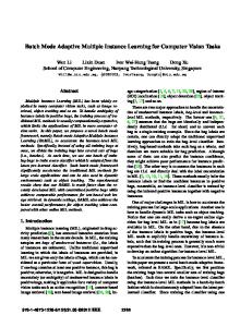
� LQT −t xlt − y lt−1 X + ult − h(t, y lt−1 ) U . (2.43) This factor is in fact an upper bound on the variation of the� function QhT −t that can � occur when “jumping” from y lt , h(t, y lt ) to xlt+1 , ult+1 . An illustration of this interpretation is given in Figure 2.1. 29
x0
x 1=f x 0 , h 0, x 0 x2
r 0 = x 0 ,h 0, x 0
0 l0
1
l0
x ,u l0
l0
l0
l0
T −1 l1
x , u , r , y
l1
l1
x
l1
x , u , r , y x
l0
x T −1
x T −2
l T −2
,u
l T −2
,r
l T −2
,y
xT
l T −1
l T −2
,u
l T −1
,r
l T −1
,y
l T −1
l0
0 =∣∣x −x 0∣∣X ∣∣u −h 0, x 0 ∣∣U , l l l l 1=∣∣ y −x ∣∣X ∣∣u −h1, y ∣ U ... 0
1
1
0
1
Figure 2.1: A graphical interpretation of the different terms composing the bound on J h (x0 ) inferred from a sequence of four-tuples (see Equation (2.45)). The bound is equal to the sum of all the rewards corresponding to this sequence of four-tuples (the terms rlt t = 0, 1, . . . , T − 1 on the figure) minus the sum of all the terms LQT −t δt .
30
Algorithm 1 An algorithm for computing from a sequence of four-tuples τ a lower bound on J h (x0 ). Inputs: An initial state x0 , A policy h, �T −1 � A sequence of four-tuples τ = (xlt , ult , rlt , y lt ) t=0 , Three constants Lf , Lρ , Lh which satisfy inequalities (2.16 - 2.18) ; Output: A lower bound on J h (x0 ); Algorithm: lb ← 0 ; y l−1 ← x0 ; for t = 0 to T −�1 do � PT −t−1 k LQT −t ← Lρ [Lf (1 + Lh )] ; k=0 � lb ← lb + rlt − LQT −t kxlt − y lt−1 kX + kult − h(t, y lt−1 )kU ; end for Return: lb.
Theorem 2.4.1 (Lower bound on J h (x0 )) Let x0 be an initial state of the system, h a policy, and τ a sequence of tuples: τ=
�
xlt , ult , rlt , y lt
��T −1 t=0
.
(2.44)
Then we have the following lower bound on J h (x0 ): T −1 X
(rlt − LQT −t δt ) ≤ J h (x0 ),
(2.45)
t=0
where
∀t ∈ {0, 1, . . . , T − 1}, δt = xlt − y lt−1 X + ult − h(t, y lt−1 ) U
(2.46)
with y l−1 = x0 . Proof. Using Proposition (2.3.2) and the Lipschitz continuity of QhT , we can write
� h � QT (x0 , u0 ) − QhT xl0 , ul0 ≤ LQ x0 − xl0 + u0 − ul0 , T X U 31
(2.47)
and, with u0 = h(0, x0 ), h � J (x0 ) − QhT xl0 , ul0 = ≤
h � QT (x0 , h(0, x0 )) − QhT xl0 , ul0 (2.48)
�
l0 l0
LQT x0 − x X + h(0, x0 ) − u U . (2.49)
It follows that � QhT xl0 , ul0 − LQT δ0 ≤ J h (x0 ).
(2.50)
By definition of the state-action evaluation function QhT , we have � � � ��� QhT xl0 , ul0 = ρ xl0 , ul0 + QhT −1 f xl0 , ul0 , h 1, f xl0 , ul0
(2.51)
and from there � � QhT xl0 , ul0 = rl0 + QhT −1 y l0 , h(1, y l0 ) .
(2.52)
� QhT −1 y l0 , h(1, y l0 ) + rl0 − LQT δ0 ≤ J h (x0 ).
(2.53)
Thus,
By using the Lipschitz continuity of the function QhT −1 , we can write h QT −1 (y l0 , h(1, y l0 )) − QhT −1 (xl1 , ul1 )
� ≤ LQT −1 y l0 − xl1 X + h(1, y l0 ) − ul1 U
(2.54)
= LQT −1 δ1 ,
(2.55)
which implies that � � QhT −1 xl1 , ul1 − LQT −1 δ1 ≤ QhT −1 y l0 , h(1, y l0 ) .
(2.56)
We have therefore � QhT −1 xl1 , ul1 + rl0 − LQT δ0 − LQT −1 δ1 ≤ J h (x0 ). By iterating this derivation, we obtain inequality (2.45).
32
(2.57)
2.5
Finding the highest lower bound
Let B h (τ, x0 ) =
T −1 X
� lt � r − LQT −t δt ,
(2.58)
t=0
with
δt = xlt − y lt−1 X + ult − h(t, y lt−1 ) U ,
(2.59)
be the function that maps a T -length sequence of four-tuples τ and the initial state of the system x0 into the lower bound on J h (x0 ) proved by Theorem 2.4.1. Let Fn T denote the set of all possible T -length sequences of four-tuples built from the elements of Fn , and let LhFn (x0 ) be defined as follows: LhFn (x0 ) = max B h (τ, x0 ) . τ ∈Fn T
(2.60)
In this section, we provide an algorithm for computing in an efficient way the value of LhFn (x0 ). A naive approach for computing this value would consist in doing an exhaustive search over all the elements of Fn T . However, as soon as the optimization horizon T grows, this approach becomes computationally impractical even if Fn has only a handful of elements. Our algorithm for computing LhFn (x0 ) is summarized in Table 2. It is in essence identical to the Viterbi algorithm [15], and we observe that its complexity is linear with respect to the optimization horizon T and quadratic with respect to the size n of the sample of four-tuples. The rationale behind this algorithm is the following. Let us first introduce some notations. Let τ (i) denote the index of the ith four-tuple of the sequence τ (τ (i) = li ), let B h (τ, x0 )(j) =
j X (rlt − LQT −t δt )
(2.61)
t=0
and let τ ∗ be a sequence of tuples such that τ ∗ ∈ arg max B h (τ, x0 ).
(2.62)
τ ∈Fn T
We have that LhFn (x0 ) = B h (τ ∗ , x0 )(T − 2) + V1 (τ ∗ (T − 1)) 33
(2.63)
where V1 is a n-dimensional vector whose i−th component is: 0
0
0
max ri − LQ1 kxi − y i kX + kui − h(T − 1, y i )kU 0 i
��
.
(2.64)
Now let use observe that: LhFn (x0 ) = B h (τ ∗ , x0 )(T − 3) + V2 (τ ∗ (T − 2))
(2.65)
where V2 is a n-dimensional vector whose ith component is: � � 0 0 0 max ri − LQ2 kxi − y i kX + kui − h(T − 2, y i )kU + V1 (i0 ) . 0 i
(2.66)
By proceeding recursively, it is therefore possible to determine the value of B h (τ ∗ , x0 ) = LhFn (x0 )
(2.67)
without having to screen all the elements of Fn T . Although this is rather evident, we want to stress the fact that LhFn (x0 ) can not decrease when new elements are added to Fn . In other words, the quality of this lower bound is monotonically increasing when new samples are collected. To quantify this behavior, we characterize in the next section the tightness of this lower bound as a function of the density of the sample of four-tuples.
2.6
Tightness of the lower bound LhFn (x0 )
In this section we study the relation of the tightness of LhFn (x0 ) with respect to the distance between the elements (x, u) ∈ X × U and the pairs (xl , ul ) formed by the two first elements of the four-tuples composing Fn . We prove in Theorem 2.6.1 that if X × U is bounded, then ∗ J h (x0 ) − LhFn (x0 ) ≤ CαF , n
(2.68)
∗ where C is a constant depending only on the control problem and where αF is the � l ln n maximum distance from any (x, u) ∈ X × U to its closest neighbor in (x , u ) l=1 . The main philosophy behind the proof is the following. First, a sequence of fourtuples whose state-action pairs (xlt , ult ) stand close to the different state-action pairs (xt , ut ) visited when the system is controlled by h is built. Then, it is shown that the lower bound B computed when considering this particular sequence is such that ∗ J h (x0 ) − B ≤ CαF . n
From there, the proof follows immediately. 34
(2.69)
Algorithm 2 A Viterbi-like algorithm for computing the highest lower bound LhFn (x0 ) (see Eqn (2.58)) over all the sequences of four-tuples τ made from elements of Fn . Inputs: An initial state x0 , A policy h, A set of four-tuples Fn = {(xl , ul , rl , y l )}nl=1 Three constants Lf , Lρ , Lh which satisfy inequalities (2.16 - 2.18) ; Output: A lower bound on J h (x0 ) equal to LhFn (x0 ) ; Algorithm: Create two n-dimensional vectors VA and VB ; VA (i) ← 0, ∀i = {1, . . . , n} ; VB (i) ← 0, ∀i = {1, . . . , n} ; for t = T − 1 to 1 do for i = 1 to n (update the value of VA ) do� � PT −t−1 LQT −t ← Lρ [Lf (1 + Lh )]k ; k=0 u ← h(t, y i ) ; � i0 i0 i i0 VA (i) ← max (r −L kx − y k +ku − uk +VB (i0 )) ; Q X U T −t 0 i
end for VB ← VA ; end for u0 ← h(0, x�0 );
i0
∗
i0
i0
lb ← max r − LQT kx − x0 kX + ku − u0 kU 0 i
�
� + VB (i ) ; 0
Return: lb∗ . Theorem 2.6.1 � n Let x0 be an initial state, h a policy, and Fn = (xl , ul , rl , y l ) l=1 a set of four-tuples. We suppose that ∃ α ∈ R+ : � � � l l sup min kx − xkX + ku − ukU ≤ α, (2.70) (x,u)∈X ×U
l∈{1,...,n}
∗ and we note αF the smallest constant which satisfies (2.70). n Then
∗ ∃ C ∈ R+ : J h (x0 ) − LhFn (x0 ) ≤ CαF . n
35
(2.71)
Proof. Let (x0 , u0 , r0 , x1 , u1 , . . . , xT −1 , uT −1 , rT −1 , xT )
(2.72)
be the trajectory of the system starting from x0 when the actions are selected ∀t ∈ � �T −1 {0, 1, . . . , T − 1} according to the policy h. Let τ = (xlt , ult , rlt , y lt ) t=0 be a sequence of four-tuples that satisfies ∀t ∈ {0, 1, . . . , T − 1},
l
x t − xt + ult − ut = X U
min l∈{1,...,n}
l
x − xt + ul − ut (2.73) U X
We have B h (τ, x0 ) =
T −1 X
� lt � r − LQT −t δt
(2.74)
t=0
where
∀t ∈ {0, 1, . . . , T − 1} , δt = xlt − y lt−1 X + ult − h(t, y lt−1 ) U . Let us focus on δt . We have that
δt = xlt − xt + xt − y lt−1 X + ult − ut + ut − h(t, y lt−1 ) U ,
(2.75)
(2.76)
and hence
δt ≤ xlt − xt X + xt − y lt−1 X + ult − ut U + ut − h(t, y lt−1 ) U . (2.77) Using inequality (2.70), we can write
l
∗
x t − xt + ult − ut ≤ αF , n X U
(2.78)
and so we have
∗ δt ≤ αF + xt − y lt−1 X + ut − h(t, y lt−1 ) U . n • On the one hand, we have
xt − y lt−1 = f (xt−1 , ut−1 ) − f (xlt−1 , ult−1 ) X X and the Lipschitz continuity of f implies that
�
xt − y lt−1 ≤ Lf xt−1 − xlt−1 + ut−1 − ult−1 . X X U 36
(2.79)
(2.80)
(2.81)
So, as
∗
xt−1 − xlt−1 + ut−1 − ult−1 ≤ αF , n X U
(2.82)
∗
xt − y lt−1 ≤ Lf αF . n X
(2.83)
we have
• On the other hand, we have
ut − h(t, y lt−1 ) = h(t, xt ) − h(t, y lt−1 ) U U
(2.84)
and the Lipschitz continuity of h implies that
ut − h(t, y lt−1 ) ≤ Lh xt − y lt−1 . U X
(2.85)
Since, according to Equation (2.83), we have
∗
xt − y lt−1 ≤ Lf αF , n X
(2.86)
we then obtain
∗
ut − h(t, y lt−1 ) ≤ Lh Lf αF . n U
(2.87)
Furthermore, (2.79), (2.83) and (2.87) imply that ∗ ∗ ∗ ∗ δt ≤ αF + Lf αF + Lh Lf αF = αF (1 + Lf (1 + Lh )) n n n n
(2.88)
and B h (τ, x0 ) ≥
T −1 X
� lt � . ∗ r − LQT −t αF (1 + Lf (1 + Lh )) = B. n
(2.89)
t=0
We also have, by definition of LhFn (x0 ), J h (x0 ) ≥ LhFn (x0 ) ≥ B h (τ, x0 ) ≥ B.
(2.90)
h J (x0 ) − LhF (x0 ) ≤ J h (x0 ) − B = J h (x0 ) − B, n
(2.91)
Thus,
37
and we have h
J (x0 ) − B
T −1 X � � � lt ∗ = rt − r + LQT −t αFn (1 + Lf (1 + Lh )) , (2.92) t=0
T −1 X
≤
� � ∗ rt − rlt + LQ αF (1 + Lf (1 + Lh )) . T −t n
(2.93)
t=0
The Lipschitz continuity of ρ allows to write � rt − rlt = ρ(xt , ut ) − ρ xlt , ult
�
≤ Lρ xt − xlt X + ut − ult U ,
(2.94) (2.95)
and using inequality (2.70), we have ∗ rt − rlt ≤ Lρ αF . n
(2.96)
Finally, we obtain J h (x0 ) − B
T −1 X
�
∗ ∗ Lρ αF + LQT −t αF (1 + Lf (1 + Lh )) n n
�
(2.97)
∗ LQT −t αF (1 + Lf (1 + Lh )) n
(2.98)
� � T −1 X � ∗ ≤ αF T L + L 1 + L (1 + L ) . ρ QT −t f h n
(2.99)
≤
t=0 ∗ ≤ T Lρ αF + n
T −1 X t=0
t=0
Thus h
J (x0 ) −
LhFn (x0 )
≤
∗ αF n
� � T −1 X � T Lρ + LQT −t 1 + Lf (1 + Lh ) ,
(2.100)
t=0
which completes the proof.
2.7
Conclusions and future research
We have introduced in this chapter an approach for deriving from a sample of trajectories a lower bound on the finite-horizon return of any policy from any given initial state. 38
We also have proposed a dynamic programming (Viterbi-like) algorithm for computing this lower bound whose complexity is linear in the optimization horizon and quadratic in the total number of state transitions of the sample of trajectories. This approach and algorithm may directly be transposed in order to compute an upper bound, so as to bracket the performance of the given policy, when applied to a given initial state. We also have derived a characterization of these bounds, in terms of the density of the coverage of the state-action space by the sample of trajectories used to compute them. This analysis shows that the lower (and upper) bound converges at least linearly towards the true value of the return with the density of the sample (measured by the maximal distance of any state-action pair to this sample). The Lipschitz continuity assumptions upon which the results have been built may seem restrictive, and they indeed are. Indeed, when facing a real-life problem, it may be difficult to establish whether its systems dynamics and reward function are indeed Lipschitz continuous. Secondly, even if one can guarantee that the Lipschitz assumptions are satisfied, it is still important to be able to establish some not too-conservative approximations of the Lipschitz constants. Indeed, the larger they are, the looser the bounds will be. In the same order of ideas, the choice of the norms on the state space and the action space might influence the value of the bounds and should thus also be chosen carefully. While the approach has been designed for computing some lower bounds on the cumulated reward obtained by a given policy, it could also serve as the base for designing new reinforcement learning algorithms which would output policies that lead to the maximization of these lower bounds. The proposed approach could also be used in combination with batch mode reinforcement learning algorithms for identifying the pieces of trajectories that influence the most the lower bounds of the RL policy and, from there, for selecting a concise set of four-tuples from which it is possible to extract a good policy. This problem is particularly important when batch mode RL algorithms are used to design autonomous intelligent agents. Indeed, after a certain time of interaction with their environment, the sample of information these agents collect may become so numerous that batch mode RL techniques may become computationally impractical [4]. Since there exist in this context many non-deterministic problems for which it would be interesting to be able to have a lower bound on the performances of a policy (e.g., those related to the inference from clinical data of decision rules for treating chronic-like diseases [11]), extending our approach to stochastic systems would certainly be relevant. Future research on this topic could follow several paths: the study of lower bounds on the expected cumulated rewards, the design of worst-case lower bounds, a study of the case where the disturbances are part of the trajectories, etc.
39
40
Bibliography [1] D. P. Bertsekas. Dynamic Programming and Optimal Control, volume 1, volume I. Athena Scientific, Belmont, MA, 3rd edition, 2005. [2] D.P. Bertsekas and J.N. Tsitsiklis. Neuro-Dynamic Programming. Athena Scientific, 1996. [3] E.F. Camacho and C. Bordons. Model Predictive Control. Springer, 2004. [4] D. Ernst. Selecting concise sets of samples for a reinforcement learning agent. In Proceedings of the Third International Conference on Computational Intelligence, Robotics and Autonomous Systems (CIRAS 2005), Singapore, 2005. [5] D. Ernst, P. Geurts, and L. Wehenkel. Tree-based batch mode reinforcement learning. Journal of Machine Learning Research, 6:503–556, 2005. [6] R. Fonteneau, S. Murphy, L. Wehenkel, and D. Ernst. Inferring bounds on the performance of a control policy from a sample of trajectories. In Proceedings of the 2009 IEEE Symposium on Adaptive Dynamic Programming and Reinforcement Learning (IEEE ADPRL 2009), Nashville, TN, USA, 2009. [7] J.E. Ingersoll. Theory of Financial Decision Making. Rowman and Littlefield Publishers, Inc., 1987. [8] M. Kearns and S. Singh. Finite-sample convergence rates for Q-learning and indirect algorithms. In Advances in Neural Information Processing Systems, pages 996–1002. MIT Press, 1999. [9] M.G. Lagoudakis and R. Parr. Least-squares policy iteration. Jounal of Machine Learning Research, 4:1107–1149, 2003. 41
[10] S.A. Murphy. Optimal dynamic treatment regimes. Journal of the Royal Statistical Society, Series B, 65(2):331–366, 2003. [11] S.A. Murphy. An experimental design for the development of adaptive treatment strategies. Statistics in Medicine, 24:1455–1481, 2005. [12] D. Ormoneit and S. Sen. Kernel-based reinforcement learning. Machine Learning, 49(2-3):161–178, 2002. [13] R.E. Schapire. On the worst-case analysis of temporal-difference learning algorithms. Machine Learning, 22(1/2/3), 1996. [14] R.S. Sutton and A.G. Barto. Reinforcement Learning. MIT Press, 1998. [15] A. Viterbi. Error bounds for convolutional codes and an asymptotically optimum decoding algorithm. IEEE Transactions on Information Theory, 13(2):260– 269, 1967.
42
Chapter 3
Towards min max generalization in reinforcement learning In this chapter, we introduce a min max approach for addressing the generalization problem in Reinforcement Learning. The min max approach works by determining a sequence of actions that maximizes the worst return that could possibly be obtained considering any dynamics and reward function compatible with the sample of trajectories and some prior knowledge on the environment. We consider the particular case of deterministic Lipschitz continuous environments over continuous state spaces, finite action spaces, and a finite optimization horizon. We discuss the non-triviality of computing an exact solution of the min max problem even after reformulating it so as to avoid search in function spaces. For addressing this problem, we propose to replace, inside this min max problem, the search for the worst environment given a sequence of actions by an expression that lower bounds the worst return that can be obtained for a given sequence of actions. This lower bound has a tightness that depends on the sample sparsity. From there, we propose an algorithm of polynomial complexity that returns a sequence of actions leading to the maximization of this lower bound. We give a condition on the sample sparsity ensuring that, for a given initial state, the proposed algorithm produces an optimal sequence of actions in open-loop. Our experiments show that this algorithm can lead to more cautious policies than algorithms combining dynamic programming with function approximators. Parts of this work have been published in the Proceedings of the International Conference on Agents and Artificial Intelligence (ICAART 2010) [13], where it received a 43
“Best Sudent Paper Award”. An extended version will be published as a book chapter by Springer [12]. This chapter is an extended version of [12]. In this chapter, we consider: • a deterministic setting, • a continuous state space and a finite action space.
44
3.1
Introduction
Since the late sixties, the field of Reinforcement Learning (RL) [28] has studied the problem of inferring from the sole knowledge of observed system trajectories, nearoptimal solutions to optimal control problems. The original motivation was to design computational agents able to learn by themselves how to interact in a rational way with their environment. The techniques developed in this field have appealed researchers trying to solve sequential decision making problems in many fields such as Finance [16], Medicine [20, 21] or Engineering [24]. RL algorithms are challenged when dealing with large or continuous state spaces. Indeed, in such cases they have to generalize the information contained in a generally sparse sample of trajectories. The dominating approach for generalizing this information is to combine RL algorithms with function approximators [2, 17, 9]. Usually, these approximators generalize the information contained in the sample to areas poorly covered by the sample by implicitly assuming that the properties of the system in those areas are similar to the properties of the system in the nearby areas well covered by the sample. This in turn often leads to low performance guarantees on the inferred policy when large state space areas are poorly covered by the sample. This can be explained by the fact that when computing the performance guarantees of these policies, one needs to take into account that they may actually drive the system into the poorly visited areas to which the generalization strategy associates a favorable environment behavior, while the environment may actually be particularly adversarial in those areas. This is corroborated by theoretical results which show that the performance guarantees of the policies inferred by these algorithms degrade with the sample sparsity where, loosely speaking, the sparsity can be seen as the radius of the largest non-visited state space area. 1 As in our previous work [13] from which this chapter is an extended version, we assume a deterministic Lipschitz continuous environment over continuous state spaces, finite action spaces, and a finite time-horizon. In this context, we introduce a min max approach to address the generalization problem. The min max approach works by determining a sequence of actions that maximizes the worst return that could possibly be obtained considering any dynamics and reward functions compatible with the sample of trajectories, and a weak prior knowledge given in the form of upper bounds on the Lipschitz constants of the environment. However, we show that finding an exact solu1 Usually, these theoretical results do not give lower bounds per se but a distance between the actual return of the inferred policy and the optimal return. However, by adapting in a straightforward way the proofs behind these results, it is often possible to get a bound on the distance between the estimate of the return of the inferred policy computed by the RL algorithm and its actual return and, from there, a lower bound on the return of the inferred policy.
45
tion of the min max problem is far from trivial, even after reformulating the problem so as to avoid the search in the space of all compatible functions. To circumvent these difficulties, we propose to replace, inside this min max problem, the search for the worst environment given a sequence of actions by an expression that lower bounds the worst return that can be obtained for a given sequence of actions. This lower bound is derived from [11] (also reported in Chapter 2) and has a tightness that depends on the sample sparsity. From there, we propose a Viterbi–like algorithm [29] for computing an open-loop sequence of actions to be used from a given initial state to maximize that lower bound. This algorithm is of polynomial computational complexity in the size of the dataset and the optimization horizon. It is named CGRL for Cautious Generalization (oriented) Reinforcement Learning since it essentially shows a cautious behavior in the sense that it computes decisions that avoid driving the system into areas of the state space that are not well enough covered by the available dataset, according to the prior information about the dynamics and reward function. Besides, the CGRL algorithm does not rely on function approximators and it computes, as a byproduct, a lower bound on the return of its open-loop sequence of decisions. We also provide a condition on the sample sparsity ensuring that, for a given initial state, the CGRL algorithm produces an optimal sequence of actions in open-loop, and we suggest directions for leveraging our approach to a larger class of problems in RL. The rest of this chapter is organized as follows. Section 3.2 briefly discusses related work. In Section 3.3, we formalize the min max approach to generalization, and we discuss its non trivial nature in Section 3.4. In Section 3.5, we exploit the results of [11] (also reported in Chapter 2) for lower bounding the worst return that can be obtained for a given sequence of actions. Section 3.6 proposes a polynomial algorithm for inferring a sequence of actions maximizing this lower bound and states a condition on the sample sparsity for its optimality. Section 3.7 illustrates the features of the proposed algorithm and Section 3.8 discusses its interest, while Section 3.9 concludes.
3.2
Related work
The min max approach to generalization followed by the CGRL algorithm results in the output of policies that are likely to drive the agent only towards areas well enough covered by the sample. Heuristic strategies have already been proposed in the RL literature to infer policies that exhibit such a conservative behavior. As a way of example, some of these strategies associate high negative rewards to trajectories falling outside of the well covered areas. Other works in RL have already developed min max strategies when the environment behavior is partially unknown [18, 4, 25]. However, these strategies usually consider problems with finite state spaces where the uncertainities come 46
from the lack of knowledge of the transition probabilities [7, 5]. In model predictive control (MPC) where the environment is supposed to be fully known [10], min max approaches have been used to determine the optimal sequence of actions with respect to the “worst case” disturbance sequence occuring [1]. The CGRL algorithm relies on a methodology for computing a lower bound on the worst possible return (considering any compatible environment) in a deterministic setting with a mostly unknown actual environment. In this, it is related to works in the field of RL which try to get from a sample of trajectories lower bounds on the returns of inferred policies [19, 23].
3.3
Problem Statement
We consider a discrete-time system whose dynamics over T stages is described by a time-invariant equation xt+1 = f (xt , ut ) t = 0, 1, . . . , T − 1,
(3.1)
where for all t, the state xt is an element of the compact state space X ⊂ RdX where RdX denotes the dX −dimensional Euclidean space and ut is an element of the finite (discrete) action space U. T ∈ N0 is referred to as the optimization horizon. An instantaneous reward rt = ρ(xt , ut ) ∈ R
(3.2)
is associated with the action ut taken while being in state xt . For every initial state x0 ∈ X and for every sequence of actions (u0 , . . . , uT −1 ) ∈ U T , the cumulated reward over T stages (also named T −stage return) is defined as Definition 3.3.1 (T −stage return of the sequence (u0 , . . . , uT −1 )) ∀(u0 , . . . , uT −1 ) ∈ U T , ∀x0 ∈ X , J u0 ,...,uT −1 (x0 ) =
T −1 X
ρ(xt , ut ) ,
(3.3)
t=0
where xt+1 = f (xt , ut ) , ∀t ∈ {0, . . . , T − 1}.
(3.4)
We assume that the system dynamics f and the reward function ρ are Lipschitz continuous: 47
Assumption 3.3.2 (Lipschitz continuity of f and ρ) There exist finite constants Lf , Lρ ∈ R such that: ∀(x, x0 ) ∈ X 2 , ∀u ∈ U, kf (x, u) − f (x0 , u)kX 0
|ρ(x, u) − ρ(x , u)|
≤ ≤
Lf kx − x0 kX , 0
Lρ kx − x kX ,
(3.5) (3.6)
where k.kX denotes the Euclidean norm over the space X . We further suppose that: Assumption 3.3.3 1. The system dynamics f and the reward function ρ are unknown, 2. A set of one-step transitions � n Fn = (xl , ul , rl , y l ) l=1 is known where each one-step transition is such that � l y = f (xl , ul ), rl = ρ(xl , ul ).
(3.7)
(3.8)
3. Each action a ∈ U appears at least once in Fn : ∀a ∈ U, ∃(x, u, r, y) ∈ Fn : u = a
(3.9)
4. Two constants Lf and Lρ satisfying the above-written inequalities are known. These constants do not necessarily have to be the smallest ones satisfying these inequalities (i.e., the Lipschitz constants). We define the set of functions LfFn (resp. LρFn ) from X × U into X (resp. into R) as follows : Definition 3.3.4 (Compatible environments) ∀x, x0 ∈ X , ∀u ∈ U , kf 0 (x, u) − f 0 (x0 , u)kX ≤ Lf kx − x0 kX , LfFn = f 0 : X × U → X , ∀l ∈ {1, . . . , n}, f 0 (xl , ul ) = f (xl , ul ) = y l (3.10) 48
LρFn
∀x, x0 ∈ X , ∀u ∈ U , |ρ0 (x, u) − ρ0 (x0 , u)| ≤ Lρ kx − x0 kX , . = ρ 0 : X × U → R ∀l ∈ {1, . . . , n}, ρ0 (xl , ul ) = ρ(xl , ul ) = rl (3.11)
In the following, we call a “compatible environment” any pair (f 0 , ρ0 ) ∈ LfFn × LρFn .
(3.12)
Given a compatible environment (f 0 , ρ0 ), a sequence of actions (u0 , . . . , uT −1 ) ∈ U T and an initial state x0 ∈ X , we introduce the (f 0 , ρ0 )−return over T stages when starting from x0 ∈ X : Definition 3.3.5 ((f 0 , ρ0 )−return over T stages) ∀(f 0 , ρ0 ) ∈ LfFn × LρFn , ∀(u0 , . . . , uT −1 ), ∀x0 ∈ X , u ,...,uT −1
J(f00 ,ρ0 )
(x0 ) =
T −1 X
ρ0 (x0t , ut ) ,
(3.13)
t=0
where x0t+1 = f 0 (x0t , ut ), ∀t ∈ {0, . . . , T − 1} ,
(3.14)
and x00 = x0 . u ,...,uT −1
We introduce IF0n
u ,...,uT −1
IF0n
(x0 ) such that
(x0 ) =
u ,...,uT −1
The existence of IF0n
min
(f 0 ,ρ0 )∈LfFn ×Lρ Fn
n o u ,...,u J(f00 ,ρ0 ) T −1 (x0 ) .
(3.15)
(x0 ) is ensured by the following arguments:
1. The space X is compact, 2. The set LfFn × LρFn is closed and bounded considering the k.k∞ norm k(f 0 , ρ0 )k∞ =
sup (x,u)∈X ×U
k(f 0 (x, u), ρ0 (x, u))kRdX +1
where k.kRdX +1 is the Euclidean norm over RdX +1 49
(3.16)
3. One can show that the mapping u ,...,uT −1
MF0n ,x0
: LfFn × LρFn → R
(3.17)
such that u ,...,uT −1
MF0n ,x0
u ,...,uT −1
(f 0 , ρ0 ) = J(f00 ,ρ0 )
(x0 )
(3.18)
is a continuous mapping. Furthermore, this also proves that ∀(u0 , . . . , uT −1 ) ∈ U T , ∀x0 ∈ X , u ,...,uT −1
∃(fFn0 ,x0 J
u ,...,uT −1
, ρF0n ,x0
u0 ,...,uT −1 u ,...,uT −1
0 (fFn ,x
0
) ∈ LfFn × LρFn : u ,...,uT −1
u ,...,uT −1
,ρF0n ,x
0
)
(x0 ) = IF0n
(x0 ).
(3.19)
Our goal is to compute, given an initial state x0 ∈ X , an open-loop sequence of actions (u˙ 0 (x0 ), . . . , u˙ T −1 (x0 )) ∈ U T that gives the highest return in the least favorable compatible environment. This problem can be formalized as the min max problem: � u0 ,...,uT −1 (u˙ 0 (x0 ), . . . , u˙ T −1 (x0 )) ∈ arg max IFn (x0 ) . (3.20) (u0 ,...,uT −1 )∈U T
3.4
Reformulation of the min max problem
Since U is finite, one could solve the min max problem by computing for each seu ,...,uT −1 quence of actions (u0 , . . . , uT −1 ) ∈ U T the value of IF0n (x0 ). As the latter computation is posed as an infinite-dimensional minimization problem over the function space LfFn × LρFn , we first show that it can be reformulated as a finite-dimensional u ,...,uT −1 problem over X T −1 × RT . This is based on the observation that IF0n (x0 ) is actually equal to the lowest sum of rewards that could be collected along a trajectory compatible with an environment from LfFn × LρFn , and is precisely stated by the following Theorem. Theorem 3.4.1 (Equivalence) u ,...,uT −1 Let (u0 , . . . , uT −1 ) ∈ U T and x0 ∈ X . Let KF0n (x0 ) be the solution of the following optimization problem: (T −1 ) X u0 ,...,uT −1 KFn (x0 ) = min rˆt , (3.21) rˆ0 . . . rˆT −1 ∈ R t=0 x ˆ0 . . . x ˆT −1 ∈ X 50
where the variables x ˆ0 , . . . , x ˆT −1 and rˆ0 , . . . , rˆT −1 satisfy the constraints
� lt Lρ x ˆt − xlt X ,
rˆt − r ≤ ∀lt ∈ {1, . . . , n|ult = ut } ,
x ˆt − xlt X ˆt+1 − y lt X ≤ Lf x (3.22) |ˆ rt − rˆt0 | ≤ Lρ kˆ xt − x ˆt0 kX , kˆ xt+1 − x ˆt0 +1 kX ≤ Lf kˆ xt − x ˆt0 kX
�
∀t, t0 ∈ {0, . . . , T − 1|ut = ut0 } , (3.23)
x ˆ 0 = x0 .
(3.24)
Then, u ,...,uT −1
KF0n
u ,...,uT −1
(x0 ) = IF0n
(x0 ) .
(3.25)
Proof. • Let us first prove that u ,...,uT −1
IF0n
u ,...,uT −1
(x0 ) ≤ KF0n
(x0 ) .
(3.26)
Let us assume that we know a set of variables x ˆ0 , . . . , x ˆT −1 and rˆ0 , . . . , rˆT −1 that are solution of the optimization problem. To each action u ∈ U, we associate the sets � Au = xl ∈ {x1 , . . . , xn }|ul = u (3.27) and Bu = {ˆ xt ∈ {ˆ x0 , . . . , x ˆT −1 }|ut = u} .
(3.28)
Let Su = Au ∪ Bu . For simplicity in the proof, we assume that the points of Su are in general position, i.e., no (dX + 1) points from Su lie in a (dX − 1)−dimensional plane (the points are affinely independent). This allows to compute a dX −dimensional triangulation {∆1 , . . . , ∆p } of the convex hull H(Su ) defined by the set of points Su [6]. We introduce for every value of u ∈ U two Lipschitz continuous functions f˜u : X → X and ρ˜u : X → R defined as follows: – Inside the convex hull H(Su ) Let guf : Su → X and guρ : Su → R be such that: ∀xl ∈ Au ,
�
guf (xl ) = f (xl , u) guρ (xl ) = ρ(xl , u)
� and ∀ˆ xt ∈ Bu \Au ,
guf (ˆ xt ) = x ˆt+1 guρ (ˆ xt ) = rˆt
. (3.29)
51
Then, we define the functions f˜u and ρ˜u inside H(Su ) as follows: ∀k ∈ {1, . . . , p}, ∀x0 ∈ ∆k , f˜u (x0 )
dX X +1
=
λki (x0 )guf (ski ) ,
(3.30)
λki (x0 )guρ (ski ) ,
(3.31)
i=1
ρ˜u (x0 )
dX X +1
=
i=1
where ski that
i = 1 . . . (dX + 1) are the vertices of ∆k and λki (x) are such x0 =
dX X +1
λki (x0 )ski
(3.32)
i=1
with dX X +1
λki (x0 ) = 1
(3.33)
λki (x0 ) ≥ 0, ∀i .
(3.34)
i=1
and
– Outside the convex hull H(Su ) According the Hilbert Projection Theorem [26], for every point x00 ∈ X , there exists a unique point y 00 ∈ H(Su ) such that kx00 −y 00 kX is minimized over H(Su ). This defines a mapping tu : X → H(Su )
(3.35)
which is 1−Lipschitzian. Using the mapping tu , we define the functions f˜u and ρ˜u outside H(Su ) as follows: ∀x00 ∈ X \H(Su ), f˜u (x00 ) 00
ρ˜u (x )
=
f˜u (tu (x00 ))
(3.36)
=
ρ˜u (tu (x00 )) .
(3.37)
We finally introduce the functions f˜ and ρ˜ over the space X × U as follows: ∀(x, u) ∈ X × U, f˜(x, u)
= f˜u (x)
(3.38)
ρ˜(x, u)
= ρ˜u (x) .
(3.39)
52
One can easily show that the pair (f˜, ρ˜) belongs to LfFn × LρFn and satisfies u ,...,uT −1
J(f˜0,ρ) ˜
(x0 )
T −1 X
=
ρ˜(ˆ xt , ut )
(3.40)
rˆt
(3.41)
t=0 T −1 X
=
t=0
with x ˆt+1 = f˜(ˆ xt , ut )
(3.42)
and x ˆ0 = x0 . This proves that u ,...,uT −1
IF0n
u ,...,uT −1
(x0 ) ≤ KF0n
(x0 ) .
(3.43)
(Note that one could still build two functions (f˜, ρ˜) ∈ LfFn × LρFn even if the sets of points (Su )u∈U are not in general position) • Then, let us prove that u ,...,uT −1
KF0n
u ,...,uT −1
(x0 ) ≤ IF0n u ,...,u
(x0 ) .
u ,...,uT −1
We consider the environment (fFn0 ,x0 T −1 , ρF0n ,x0 (3.19) at the end of Section 3.3. One has u ,...,uT −1
IF0n
(x0 )
= J =
(3.44)
) introduced in Equation
u0 ,...,uT −1 u ,...,uT −1
0 (fFn ,x
T −1 X
0
u ,...,uT −1
,ρF0n ,x
0
r˜t ,
)
(x0 )
(3.45) (3.46)
t=0
with, ∀t ∈ {0, . . . , T − 1} , r˜t x ˜t+1 x ˜0
u ,...,uT −1
= ρF0n ,x0
(3.47)
=
(3.48)
(˜ xt , ut ) , u0 ,...,uT −1 fFn ,x0 (˜ xt , ut ) ,
= x0 .
(3.49)
The variables x ˜0 , . . . , x ˜T −1 and r˜0 , . . . , r˜T −1 satisfy the constraints introduced in Theorem (3.4.1). This proves that u ,...,uT −1
KF0n
u ,...,uT −1
(x0 ) ≤ IF0n
and completes the proof.
53
(x0 )
(3.50)
Unfortunately, this latter minimization problem turns out to be non-convex in its generic form and, hence “off the shelf” algorithms will only be able to provide upper bounds on its value. Furthermore, the overall complexity of an algorithm that would be based on the enumeration of U T , combined with a local optimizer for the inner loop, may be intractable as soon as the cardinality of the action space U and/or the optimization horizon T become large. We leave the exploration of the above formulation for future research. Instead, in the following subsections, we use the results from [11] (reported in Chapter 2) to define a maximal lower bound u ,...,uT −1
LF0n
u ,...,uT −1
(x0 ) ≤ IF0n
(x0 )
(3.51)
for a given initial state x0 ∈ X and a sequence (u0 , . . . , uT −1 ) ∈ U T . Furthermore, u ,...,uT −1 we show that the maximization of this lower bound LF0n (x0 ) with respect to the choice of a sequence of actions lends itself to a dynamic programming type of decomposition. In the end, this yields a polynomial algorithm for the computation of a ˜∗Fn ,T −1 (x0 )) maximizing a lower bound of the sequence of actions (˜ u∗Fn ,0 (x0 ), . . . , u original min max problem, i.e. � u0 ,...,uT −1 LFn (x0 ) . (3.52) (˜ u∗Fn ,0 (x0 ), . . . , u ˜∗Fn ,T −1 (x0 )) ∈ arg max (u0 ,...,uT −1 )∈U T
3.5
Lower bound on the return of a given sequence of actions
In this section, we present a method for computing, from a given initial state x0 ∈ X , a sequence of actions (u0 , . . . , uT −1 ) ∈ U T , a dataset of transitions, and weak prior u ,...,uT −1 (x0 ). The method is knowledge about the environment, a lower bound on IF0n T adapted from [11] (reported in Chapter 2). In the following, we denote by Fn,(u 0 ,...,uT −1 ) the set of all sequences of T one-step system transitions that may be built from elements of Fn and that are compatible with (u0 , . . . , uT −1 ): Definition 3.5.1 (Compatible sequences of transitions) ∀(u0 , . . . , uT −1 ) ∈ U T , � � l0 l0 l0 l0 � �� T Fn,(u = x , u , r , y , . . . , xlT −1 , ulT −1 , rlT −1 , y lT −1 0 ,...,uT −1 ) � (3.53) ult = ut , ∀t ∈ {0, . . . , T − 1} 54
x0
x 1=f ' x 0 ,u 0 x2
r 0 = ' x 0 , u0
x T −1
x T −2
xT
l0
∥x 0 −x ∥X l0
l0
l0
l0
l0
l1
∥y −x ∥X
l0
x ,u l0
x , u , r , y
l1
l1
∥y l1
l T −2
l T −1
−x ∥X
l1
x , u , r , y x
lt
l T −2
,u
l T −2
,r
l T −2
x
,y
l T −1
l T −2
,u
l T −1
,r
l T −1
,y
l T −1
∀ t ∈{ 0,... ,T −1 } , u =u t T −1
u l l l l J u f ',..., , ' x 0 ≥ ∑ [r − LQ ∥ y −x ∥X ] with y = x 0 0
T −1
t
t=0
t−1
t
−1
T −t
1
Figure 3.1: A graphical interpretation of the different terms composing the bound on u ,...,u J(f00 ,ρ0 ) T −1 (x0 ) computed from a sequence of one-step transitions.
55
u ,...,u
T −1 First, we compute a lower bound on IF0n (x0 ) from any given element τ from T Fn,(u0 ,...,uT −1 ) . This lower bound B(τ, x0 ) is made of the sum of the T rewards corPT −1 responding to τ ( t=0 rlt ) and T negative terms. Every negative term is associated with a one-step transition. More specifically, the negative term corresponding to the transition (xlt , ult , rlt , y lt ) of τ represents an upper bound on the variation of the cumulated rewards over the remaining time steps that can occur by simulating the system from a state xlt rather than y lt−1 (with y l−1 = x0 ) and considering any compatible T environment (f 0 , ρ0 ) from LfFn × LρFn . By maximizing B(τ, x0 ) over Fn,(u , 0 ,...,uT −1 ) u0 ,...,uT −1 we obtain a maximal lower bound on IFn (x0 ). Furthermore, we prove that the distance from the maximal lower bound to the actual return J u0 ,...,uT −1 (x0 ) can be characterized in terms of the sample sparsity.
3.5.1
Computing a bound from a given sequence of one-step transitions
We have the following lemma. Lemma 3.5.2 Let (u0 , . . . , uT −1 ) ∈ U T be a sequence of actions and x0 ∈ X an initial state. Let τ be a sequence of one-step transitions: τ=
�
xlt , ult , rlt , y lt
��T −1
T ∈ Fn,(u . 0 ,...,uT −1 )
(3.54)
(x0 ) ≤ J u0 ,...,uT −1 (x0 ) ,
(3.55)
t=0
Then, u ,...,uT −1
B(τ, x0 ) ≤ IF0n with
T −1
� . X � lt B(τ, x) = r − LQT −t y lt−1 − xlt X ,
(3.56)
t=0
y l−1 = x0 , LQT −t = Lρ
(3.57) TX −t−1
(Lf )i .
(3.58)
i=0
Before proving Lemma 3.5.2, we prove a preliminary result related to the Lipschitz continuity of state-action value functions. 56
For any compatible environment (f 0 , ρ0 ) ∈ LfFn × LρFn , and for N = 1, . . . , T , let us define the family of (f 0 , ρ0 )−state-action value functions u ,...,u
0 T −1 :X ×U →R QN,(f 0 ,ρ0 )
(3.59)
as follows: Definition 3.5.3 ((f 0 , ρ0 )−state-action value functions) ∀(f 0 , ρ0 ) ∈ LfFn × LρFn , ∀N ∈ {1, . . . , T }, ∀(x, u) ∈ X × U, u0 ,...,uT −1 QN,(f (x, u) 0 ρ0 )
T −1 X
0
ρ0 (x0t , ut ),
(3.60)
x0t+1 = f 0 (x0t , ut ), ∀t ∈ {T − N + 1, . . . , T − 1} ,
(3.61)
x0T −N +1 = f 0 (x, u).
(3.62)
= ρ (x, u) +
t=T −N +1
where
and
u ,...,u
0 T −1 QN,(f (x, u) gives the sum of rewards from instant t = T − N to instant T − 1 0 ,ρ0 ) given the compatible environment (f 0 , ρ0 ) when
• The system is in state x ∈ X at instant T − N , • The action chosen at instant T − N is u, • The actions chosen at instants t > T − N are ut . We have the following trivial propositions: Proposition 3.5.4 ∀(f 0 , ρ0 ) ∈ LfFn × LρFn , ∀x0 ∈ X , u ,...,uT −1
J(f00 ,ρ0 )
u ,...,u
0 T −1 (x0 ) = QT,(f (x0 , u0 ). 0 ,ρ0 )
(3.63)
Proposition 3.5.5 ∀(f 0 , ρ0 ) ∈ LfFn × LρFn , ∀(x, u) ∈ X × U, ∀N ∈ {1, . . . , T − 1} u ,...,u
u ,...,u
0 −1 T −1 0 QN0+1,(fT0 ,ρ (f 0 (x, u), uT −N ) . 0 ) (x, u) = ρ (x, u) + QN,(f 0 ,ρ0 )
57
(3.64)
u ,...,u
0 T −1 ) Lemma 3.5.6 (Lipschitz continuity of QN,(f 0 ,ρ0 )
∀(f 0 , ρ0 ) ∈ LfFn × LρFn , ∀N ∈ {1, . . . , T }, ∀(x, x0 ) ∈ X 2 , ∀u ∈ U , u0 ,...,uT −1 u0 ,...,uT −1 (x0 , u) ≤ LQN kx − x0 kX , QN,(f 0 ,ρ0 ) (x, u) − QN,(f 0 ,ρ0 )
(3.65)
with LQN = Lρ
N −1 X
(Lf )i .
(3.66)
i=0
Proof. Let ∀(f 0 , ρ0 ) ∈ LfFn × LρFn be a compatible environment. We consider the statement H(N ): ∀(x, x0 ) ∈ X 2 , ∀u ∈ U, u0 ,...,uT −1 u0 ,...,uT −1 0 (x , u) (3.67) QN,(f 0 ,ρ0 ) (x, u) − QN,(f ≤ LQN kx − x0 kX . 0 ,ρ0 ) We prove by induction that H(N ) is true ∀N ∈ {1, . . . , T }. For the sake of clarity, we use the notation u0 ,...,uT −1 u0 ,...,uT −1 (x0 , u) = ∆N . (3.68) QN,(f 0 ,ρ0 ) (x, u) − QN,(f 0 ,ρ0 ) • Basis (N = 1) : We have ∆1 = |ρ0 (x, u) − ρ0 (x0 , u)| , 0
and since ρ ∈
LρFn ,
(3.69)
we can write ∆1 ≤ Lρ kx − x0 kX .
(3.70)
This proves H(1). • Induction step: We suppose that H(N ) is true, 1 ≤ N ≤ T − 1. Using Proposition (3.5.5), we can write u ,...,u −1 u0 ,...,uT −1 0 ∆N +1 = QN0+1,(fT0 ,ρ (x, u) − Q (x , u) (3.71) 0) N +1,(f 0 ,ρ0 ) 0 u0 ,...,uT −1 = ρ (x, u) − ρ0 (x0 , u) + QN,(f (f 0 (x, u), uT −N ) 0 ,ρ0 ) u0 ,...,uT −1 − QN,(f (f 0 (x0 , u), uT −N ) (3.72) 0 ,ρ0 ) and, from there, ∆N +1 ≤ ρ0 (x, u) − ρ0 (x0 , u) u0 ,...,uT −1 0 u0 ,...,uT −1 0 0 + QN,(f (f (x, u), u ) − Q (f (x , u), u ) 0 ,ρ0 ) T −N T −N . N,(f 0 ,ρ0 ) (3.73) 58
H(N ) and the Lipschitz continuity of ρ0 give ∆N +1 ≤ Lρ kx − x0 kX + LQN kf 0 (x, u) − f 0 (x0 , u)kX .
(3.74)
Since f 0 ∈ LfFn , the Lipschitz continuity of f 0 gives ∆N +1 ≤ Lρ kx − x0 kX + LQN Lf kx − x0 kX ,
(3.75)
∆N +1 ≤ LQN +1 kx − x0 kX
(3.76)
LQN +1 = Lρ + LQN Lf .
(3.77)
and then
since
This proves H(N + 1) and ends the proof.
Proof of Lemma 3.5.2. • The inequality u ,...,uT −1
IF0n
(x0 ) ≤ J u0 ,...,uT −1 (x0 )
(3.78)
is trivial since (f, ρ) belongs to LfFn × LρFn . • Let (f 0 , ρ0 ) ∈ LfFn × LρFn be a compatible environment. By assumption we have ul0 = u0 , then we use Proposition (3.5.4) and the Lipschitz continuity of u0 ,...,uT −1 QT,(f to write 0 ,ρ0 )
� u0 ,...,uT −1 u0 ,...,uT −1 (x0 ) − QT,(f xl0 , u0 ≤ LQT x0 − xl0 X . J(f 0 ,ρ0 ) 0 ,ρ0 )
(3.79)
It follows that
� u0 ,...,uT −1 u ,...,u QT,(f xl0 , u0 − LQT x0 − xl0 X ≤ J(f00 ,ρ0 ) T −1 (x0 ). 0 ,ρ0 )
(3.80)
According to Proposition (3.5.5), we have � � � u0 ,...,uT −1 u ,...,u 0 l0 QT,(f xl0 , u0 = ρ0 xl0 , u0 + QT0−1,(fT0 ρ−1 (3.81) 0 ,ρ0 ) 0 ) f (x , u0 ), u1 59
and from there � � u0 ,...,uT −1 QT,(f xl0 , u0 = rl0 + QhT −1,(f 0 ,ρ0 ) y l0 , u1 . 0 ,ρ0 )
(3.82)
Thus,
� u ,...,u u ,...,u −1 l0 l0 − LQT x0 − xl0 X ≤ J(f00 ,ρ0 ) T −1 (x0 ). (3.83) QT0−1,(fT0 ,ρ 0 ) y , u1 + r u ,...,u
−1 l1 The Lipschitz continuity of QT0−1,(fT0 ,ρ gives 0 ) with u1 = u
� � u0 ,...,uT −1 l0 u ,...,u −1 l1 l1 ≤ LQT −1 y l0 − xl1 X . QT −1,(f 0 ,ρ0 ) y , u1 − QT0−1,(fT0 ,ρ 0) x , u
(3.84) This implies that
l
� � u ,...,u −1 l1
y 0 − xl1 ≤ Qu0 ,...,uT0 −10 y l0 , u1 . QT0−1,(fT0 ,ρ 0 ) x , u1 − LQT −1 T −1,(f ,ρ ) X (3.85) We have therefore � u ,...,u −1 l1 l0 QT0−1,(fT0 ,ρ 0 ) x , u1 + r
− LQT x0 − xl0 X − LQT −1 y l0 − xl1 X u ,...,uT −1
≤ J(f00 ,ρ0 )
(x0 ).
(3.86)
� lt � r − LQT −t ky lt−1 − xlt kX .
(3.87)
By developing this iteration, we obtain u ,...,uT −1
J(f00 ,ρ0 )
(x0 ) ≥
T −1 X t=0
The right side of Equation (3.87) does not depend on the choice of (f 0 , ρ0 ) ∈ LfFn × LρFn ; Equation (3.87) is thus true for a compatible environment (f 0 , ρ0 ) such that u ,...,uT −1
(f 0 , ρ0 ) = (fFn0 ,x0
u ,...,uT −1
, ρF0n ,x0
).
(3.88)
(cf. Equation (3.19) in Section 3.3). This finally gives u ,...,uT −1
IF0n
(x0 ) ≥
T −1 X
� � lt r − LQT −t y lt−1 − xlt X
(3.89)
t=0
since u ,...,uT −1
IF0n
(x0 ) = J
u0 ,...,uT −1 u ,...,uT −1 u ,...,u ,ρF0n ,x T −1 ) 0 0
0 (fFn ,x
60
(x0 ) .
(3.90)
u ,...,u
T −1 The lower bound on IF0n (x0 ) derived in this lemma can be interpreted as follows. Given any compatible environment (f 0 , ρ0 ) ∈ LfFn × LρFn , the sum of the rewards of the “broken” trajectory formed by the sequence of one-step system transitions u ,...,u τ can never be greater than J(f00 ,ρ0 ) T −1 (x0 ), provided that every reward rlt is penal
l ized by a factor LQT −t y t−1 − xlt X . This factor is in fact an upper bound on the variation of the (T − t)-state-action value function given environment � any compatible � (f 0 , ρ0 ) that can occur when “jumping” from y lt−1 , ut to xlt , ut . An illustration of this is given in Figure 3.1.
3.5.2
Tightness of highest lower bound over all compatible sequences of one-step transitions
We define the highest lower bound over all compatible sequences of one-step transitions: Definition 3.5.7 (Highest lower bound) ∀x0 ∈ X , u ,...,uT −1
LF0n
(x0 ) =
max
T τ ∈Fn,(u
B(τ, x0 ) .
(3.91)
0 ,...,uT −1 )
u ,...,u
T −1 We analyze in this subsection the distance from the lower bound LF0n (x0 ) to the u0 ,...,uT −1 (x0 ) as a function of the sample sparsity. The sample sparsity actual return J is defined as follows:
Definition 3.5.8 (Sample sparsity) Let a ∈ U, and let Fn,a be defined as follows: � � Fn,a = xl , ul , rl , y l ∈ Fn |ul = a
(3.92)
(∀a, Fn,a 6= ∅ since each action a appears at least once in Fn ). Since X is a compact subset of RdX , it is bounded and there exists α ∈ R+ : � �
� l
x − x0 ∀a ∈ U , sup min ≤α. (3.93) X x0 ∈X
(xl ,ul ,r l ,y l )∈Fn,a
The smallest α which satisfies equation (3.93) is named the sample sparsity and is ∗ denoted by αF . n We have the following theorem. 61
Theorem 3.5.9 (Tightness of highest lower bound) ∃ C > 0 : ∀x0 ∈ X , ∀(u0 , . . . , uT −1 ) ∈ U T , u ,...,uT −1
J u0 ,...,uT −1 (x0 ) − LF0n
∗ (x0 ) ≤ CαF . n
(3.94) Proof. Let (x0 , u0 , r0 , x1 , u1 , . . . , xT −1 , uT −1 , rT −1 , xT )
(3.95)
be the trajectory of an agent starting from x0 = x when following the open-loop policy u0 , . . . , uT −1 under the (actual) environment (f, ρ). Using equation (3.93), we define the sequence of transitions τ : (3.96)
l
∗
x − xt ≤ αF . n X
(3.97)
� � lt r − LQT −t y lt−1 − xlt X
(3.98)
with y l−1 = x0 . Let us focus on y lt−1 − xlt X . We have
l
y t−1 − xlt = xlt − xt + xt − y lt−1 , X X
(3.99)
�
xlt , ult , rlt , y lt
��T −1
T ∈ Fn,(u 0 ,...,uT −1 )
τ=
that satisfies ∀t ∈ {0, 1, . . . , T − 1}
l
x t − xt = min X
t=0
l∈{1,...,n}
We have B(τ, x0 ) =
T −1 X t=0
and hence
l
y t−1 − xlt ≤ xlt − xt + xt − y lt−1 . X X X Using inequality (3.97), we can write
l
∗
y t−1 − xlt ≤ αF + xt − y lt−1 X . n X
(3.100)
(3.101)
For t = 0, one has
xt − y lt−1 X
=
kx0 − x0 kX
(3.102)
=
0.
(3.103)
62
For t > 0,
�
xt − y lt−1 = f (xt−1 , ut−1 ) − f xlt−1 , ut−1 X X and the Lipschitz continuity of f implies that
xt − y lt−1 ≤ Lf xt−1 − xlt−1 . X X
(3.104)
(3.105)
So, as ∗ kxt−1 − xlt−1 kX ≤ αF , n
(3.106)
∗ ∀t > 0, xt − y lt−1 X ≤ Lf αF . n
(3.107)
we have
Equations (3.101) and (3.107) imply that for t > 0,
l
∗
y t−1 − xlt ≤ αF (1 + Lf ) n X
(3.108)
and, for t = 0,
l
∗ ∗
y −1 − xl0 ≤ αF ≤ αF (1 + Lf ) . n n X
(3.109)
This gives B(τ, x0 ) ≥
T −1 X
� lt � . ∗ r − LQT −t αF (1 + Lf ) = B . n
(3.110)
t=0
We also have, by definition of Lu0 ,...,uT −1 (x0 ) , J u0 ,...,uT −1 (x0 ) ≥ Lu0 ,...,uT −1 (x0 ) ≥ B(τ, x0 ) ≥ B .
(3.111)
Thus, |J u0 ,...,uT −1 (x0 ) − Lu0 ,...,uT −1 (x0 )| ≤ |J u0 ,...,uT −1 (x0 ) − B|
(3.112)
u0 ,...,uT −1
=J (x0 ) − B −1 TX � � � lt ∗ = rt − r + LQT −t αFn (1 + Lf )
(3.113) (3.114)
t=0
≤
T −1 X
� rt − rlt + LQ
T −t
t=0
63
� ∗ αF (1 + Lf ) . n
(3.115)
The Lipschitz continuity of ρ allows to write � rt − rlt = ρ(xt , ut ) − ρ xlt , ut
≤ Lρ xt − xlt X ,
(3.116) (3.117)
and using inequality (3.97), we have 0 ∗ rt − rlt ≤ Lρ αF . n
(3.118)
Finally, we obtain J u0 ,...,uT −1 (x0 ) − B
≤
T −1 X
� � ∗ ∗ Lρ αF + LQT −t αF (1 + Lf ) n n
(3.119)
t=0 ∗ ≤ T Lρ αF + n
T −1 X
∗ LQT −t αF (1 + Lf ) n
(3.120)
t=0
≤
∗ αF n
T Lρ +
T −1 X
! LQT −t (1 + Lf ) .
(3.121)
t=0
Thus T −1 � � X ∗ J u0 ,...,uT −1 (x0 ) − Lu0 ,...,uT −1 (x0 ) ≤ T Lρ + (1 + Lf ) LQT −t αF , n t=0
(3.122) which completes the proof. u ,...,u
T −1 The lower bound LF0n (x0 ) thus converges to the T −stage return of the se∗ quence of actions (u0 , . . . , uT −1 ) ∈ U T when the sample sparsity αF decreases to n zero.
3.6
Computing a sequence of actions maximizing the highest lower bound
Let L∗Fn (x0 ) be the set of sequences of actions maximizing the highest lower bound: Definition 3.6.1 (Sequences of actions maximizing the highest lower bound) � u0 ,...,uT −1 ∀x0 ∈ X , L∗Fn (x0 ) = arg max LFn (x0 ) . (3.123) (u0 ,...,uT −1 )∈U T
64
The CGRL algorithm computes for each initial state x0 ∈ X a sequence of actions (˜ u∗Fn ,0 (x0 ), . . . , u ˜∗Fn ,T −1 (x0 )) that belongs to L∗Fn (x0 ). From what precedes, it fol∗ ∗ lows that the actual return J u˜Fn ,0 (x0 ),...,˜uFn ,T −1 (x0 ) (x0 ) of this sequence is lowerbounded as follows: u ,...,uT −1
max
(u0 ,...,uT −1 )∈U T
LF0n
∗
∗
(x0 ) ≤ J u˜Fn ,0 (x0 ),...,˜uFn ,T −1 (x0 ) (x0 ) .
(3.124)
u ,...,u
T −1 Due to the tightness of the lower bound LF0n (x0 ), the value of the return which ∗ is guaranteed will converge to the true return of the sequence of actions when αF n decreases to zero. Additionally, we prove in Section 3.6.1 that when the sample sparsity ∗ αF decreases below a particular threshold, the sequence n
(˜ u∗Fn ,0 (x0 ), . . . , u ˜∗Fn ,T −1 (x0 )) ∈ U T
(3.125)
is optimal. To identify a sequence of actions that belongs to L∗Fn (x0 ) without comu ,...,uT −1 puting for all sequences (u0 , . . . , uT −1 ) ∈ U T the value LF0n (x0 ), the CGRL algorithm exploits the fact that the problem of finding an element of L∗Fn (x0 ) can be reformulated as a shortest path problem.
3.6.1
Convergence of (˜ u∗Fn ,0 (x0 ), . . . , u˜∗Fn ,T −1 (x0 )) towards an optimal sequence of actions
∗ gets lower than a particular threshold, the CGRL We prove hereafter that when αF n algorithm can only output optimal policies.
Theorem 3.6.2 (Convergence of the CGRL algorithm) Let x0 ∈ X . Let � J∗ (x0 ) = (u0 , . . . , uT −1 ) ∈ U T |J u0 ,...,uT −1 (x0 ) = J ∗ (x0 ) ,
(3.126)
and let us suppose that J∗ (x0 ) 6= U T
(3.127)
(if J∗ (x0 ) = U T , the search for an optimal sequence of actions is indeed trivial). We define �(x0 ) =
min
(u0 ,...,uT −1 )∈U T \J∗ (x0 )
{J ∗ (x0 ) − J u0 ,...,uT −1 (x0 )} .
(3.128)
Then ∗ < �(x0 ) =⇒ (˜ u∗Fn ,0 (x0 ), . . . , u CαF ˜∗Fn ,T −1 (x0 )) ∈ J∗ (x0 ) . n
65
(3.129)
1
1
1
1
x ,u ,r , y
x 1 , u 1 , r 1 , y 1
1
1
1
1
x ,u ,r , y
c 1 1,2
c 0 0,1
x0
c 1 1,1
c 1 1, n
c 0 0,2
c T −1 i, j
c 1 2,1 x 2 , u 2 , r 2 , y 2
c 1 2,2 c 1 2, n c 1 n , 1
c 0 0,n
x n , un , r n , y n
c 1 n , 2 c 1 n , n
x 2 , u 2 , r 2 , y 2
x 2 , u 2 , r 2 , y 2
x n , un , r n , y n
x n , un , r n , y n
l ✶0 ,... , l ✶T−1 ∈argmax c 0 0, l 0 c1 l 0, l 1 ...c T −1 l T−2 ,l T−1 l 0 , ...,l T −1
with c t i , j=−LQ
T −t
∥ y i −x j∥X r j
✶ 0
, y 0= x 0
n
n
Figure 3.2: A graphical interpretation of the CGRL algorithm.
66
✶ T −1
u ✶F ,0 x 0 , ... , u ✶F , T−1 x 0 =u l , ... ,u l
Proof. Let us prove that by Reductio ad absurdum. Let us suppose that the algorithm does not return an optimal sequence of actions, which means that ∗
∗
J u˜Fn ,0 (x0 ),...,˜uFn ,T −1 (x0 ) (x0 ) ≤ J ∗ (x0 ) − �(x0 ) .
(3.130)
Let us consider a sequence u∗0 (x0 ), . . . , u∗T −1 (x0 ) such that (u∗0 (x0 ), . . . , u∗T −1 (x0 )) ∈ J∗ (x0 ) .
(3.131)
Then, ∗
∗
J u0 (x0 ),...,uT −1 (x0 ) (x0 ) = J ∗ (x0 ). ∗
(3.132)
∗
The lower bound Lu0 (x0 ),...,uT −1 (x0 ) (x0 ) satisfies the relationship ∗
∗
∗ J ∗ (x0 ) − Lu0 (x0 ),...,uT −1 (x0 ) (x0 ) ≤ CαF . n
(3.133)
∗ CαF < �(x0 ), n
(3.134)
Lu0 (x0 ),...,uT −1 (x0 ) (x0 ) > J ∗ (x0 ) − �(x0 ).
(3.135)
Knowing that
we have ∗
∗
By definition of �(x0 ), ∗
∗
J ∗ (x0 ) − �(x0 ) ≥ J u˜Fn ,0 (x0 ),...,˜uFn ,T −1 (x0 ) (x0 ),
(3.136)
and since ∗
∗
∗
∗
J u˜Fn ,0 (x0 ),...,˜uFn ,T −1 (x0 ) (x0 ) ≥ Lu˜Fn ,0 (x0 ),...,˜uFn ,T −1 (x0 ) (x0 ),
(3.137)
we have ∗
∗
∗
∗
Lu0 (x0 ),...,uT −1 (x0 ) (x0 ) > Lu˜Fn ,0 (x0 ),...,˜uFn ,T −1 (x0 ) (x0 ) ,
(3.138)
which contradicts the fact that the algorithm returns the sequence that leads to the highest lower bound.
67
3.6.2
Cautious Generalization Reinforcement Learning algorithm
The CGRL algorithm computes an element of the set L∗Fn (x0 ) defined previously. Definition 3.6.3 Let D : FnT → U T
(3.139)
be the operator that maps a sequence of one-step system transitions � �T −1 τ = (xlt , ult , rlt , y lt ) t=0 ∈ FnT
(3.140)
into the sequence of actions (ul0 , . . . , ulT −1 ): � �T −1 ∀τ = (xlt , ult , rlt , y lt ) t=0 ,
D(τ ) = (ul0 , . . . , ulT −1 ) .
(3.141)
Using this operator, we can write ∀x0 ∈ X , ( L∗Fn (x0 )
=
) ∃τ ∈ arg max {B(τ, x0 )} , T τ ∈Fn . (u0 , . . . , uT −1 ) ∈ U D(τ ) = (u , . . . , u 0 T −1 ) (3.142) T
Or, equivalently ∀x0 ∈ X , L∗Fn (x0 ) = � PT −1 � lt ∃τ ∈ arg max t=0 r − LQT −t ky lt−1 − xlt kX , T τ ∈Fn (u0 , . . . , uT −1 ) ∈ U T . D(τ ) = (u , . . . , u 0 T −1 ) (3.143)
From this expression, we can notice that a sequence of one-step transitions τ such that D(τ ) belongs to L∗Fn (x0 ) can be obtained by solving a shortest path problem on the graph given in Figure 3.2. The CGRL algorithm works by solving this problem using the Viterbi algorithm and by applying the operator D to the sequence of one-step transitions τ corresponding to its solution. Its complexity is quadratic with respect to the cardinality n of the input sample Fn and linear with respect to the optimization horizon T . 68
3.7
Illustration
x0
Goal
Figure 3.3: The puddle world benchmark. In this section, we illustrate the CGRL algorithm on a variant of the puddle world benchmark introduced in [27]. In this benchmark, a robot whose goal is to collect high cumulated rewards navigates on a plane. A puddle stands in between the initial position of the robot and the high reward area. If the robot is in the puddle, it gets highly negative rewards. An optimal navigation strategy drives the robot around the puddle to reach the high reward area. Two datasets of one-step transitions have been used in our example. The first set F contains elements that uniformly cover the area of the state space that can be reached within T steps. The set F 0 has been obtained by removing from F the elements corresponding to the highly negative rewards.2 2 Although
this problem might be treated by on-line learning methods, in some settings - for whatever reason - on-line learning may be impractical and all one will have is a batch of trajectories
69
Figure 3.4: CGRL with F.
The full specification of the puddle world benchmark and the exact procedure for generating F and F 0 is the following. The state space X is X = R2 .
(3.144)
The action space U is given by U = { 0.1
� 0 , −0.1
� 0 , 0
� 0.1 , 0
� −0.1 }.
(3.145)
The system dynamics f is defined as follows: f (x, u) = x + u ,
(3.146)
ρ(x, u) = k1 Nµ1 ,Σ1 (x) − k2 Nµ2 ,Σ2 (x) − k3 Nµ3 ,Σ3 (x) ,
(3.147)
and the reward function ρ:
70
Figure 3.5: FQI with F. where 0 −(x−µ)Σ−1 (x−µ) 1 2 p e , 2π |Σ| � µ1 = 1 1 , � µ2 = 0.225 0.75 , � µ3 = 0.45 0.6 , � � 0.005 0 Σ1 = , 0 0.005 � � 0.05 0 Σ2 = , 0 0.001 � � 0.001 0 Σ3 = , 0 0.05
Nµ,Σ (x) =
(3.148) (3.149) (3.150) (3.151) (3.152) (3.153) (3.154)
and k1 = 1, k2 = k3 = 20.
(3.155)
The Lipschitz constants Lf and Lρ are Lf = 1, Lρ = 1.3742 ∗ 106 . 71
(3.156)
The time horizon T is set to T = 25, and the initial state of the system to x0 = (0.35, 0.65).
(3.157)
The sets of one-step system transitions are F= � � � x ∈ −2.15 + (x, u, ρ(x, u), f (x, u))
5i , −1.85 203
+ u∈U
5j 203
�
|i, j = 1 : 203
�� , (3.158)
F 0 = F\ {(x, u, r, y) ∈ F1 |x ∈ [0.4, 0.5] × [0.25, 0.95] ∪ [−0.1, 0.6] × [0.7, 0.8]} . (3.159)
Figure 3.6: CGRL with F 0 . On Figure 3.4, we have drawn the trajectory of the robot when following the sequence of actions computed by the CGRL algorithm. Every state encountered is represented by a white square. The plane upon which the robot navigates has been colored such that the darker the area, the smaller the corresponding rewards are. In particular, the puddle area is colored in dark grey/black. We see that the CGRL policy drives the robot around the puddle to reach the high-reward area − which is represented by the 72
Figure 3.7: FQI with F 0 . light-grey circles. The CGRL algorithm also computes a lower bound on the cumulated rewards obtained by this action sequence. Here, we found out that this lower bound was rather conservative. Figure 3.5 represents the policy inferred from F by using the (finite-time version of the) Fitted Q Iteration algorithm (FQI) combined with extremely randomized trees as function approximators [9] (the FQI algorithm is also described in Appendix A). The FQI algorithm combined with extremely randomized trees is run using its default parameters given in [9]. The trajectories computed by the CGRL and FQI algorithms are very similar and so are the sums of rewards obtained by following these two trajectories. However, by using F 0 rather that F, the CGRL and FQI algorithms do not lead to similar trajectories, as it is shown on Figures 3.6 and 3.7. Indeed, while the CGRL policy still drives the robot around the puddle to reach the high reward area, the FQI policy makes the robot cross the puddle. In terms of optimality, this latter navigation strategy is much worse. The difference between both navigation strategies can be explained as follows. The FQI algorithm behaves as if it were associating to areas of the state space that are not covered by the input sample, the properties of the elements of this sample that are located in the neighborhood of these areas. This in turn explains why it computes a policy that makes the robot cross the puddle. The same behavior could probably be observed by using other algorithms that combine dynamic programming strategies with kernel-based approximators or averagers [3, 15, 22]. The CGRL 73
algorithm generalizes the information contained in the dataset, by assuming, given the initial state, the most adverse behavior for the environment according to its weak prior knowledge about the environment. This results in the fact that the CGRL algorithm penalizes sequences of decisions that could drive the robot in areas not well covered by the sample, and this explains why the CGRL algorithm drives the robot around the puddle when run with F 0 .
3.8
Discussion
The CGRL algorithm outputs a sequence of actions as well as a lower bound on its return. When Lf > 1 (e.g. when the system is unstable), this lower bound will decrease exponentially with T . This may lead to very low performance guarantees when the optimization horizon T is large. However, one can also observe that the terms LQT −t − which are responsible for the exponential decrease of the lower bound with the optimization horizon − are multiplied by the distance between the end state of a one-step transition and the beginning state of the next one-step transition of the sequence τ ∗ ∗ (ky lt−1 − xlt kX ) solution of the shortest path problem of Figure 3.2. Therefore, if ∗ ∗ these states y lt−1 and xlt are close to each other, the CGRL algorithm can lead to good performance guarantees even for large values of T . It is also important to notice that ∗ , but depends this lower bound does not depend explicitly on the sample sparsity αF n rather on the initial state for which the sequence of actions is computed. Therefore, this may lead to cases where the CGRL algorithm provides good performance guarantees for some specific initial states, even if the sample does not cover every area of the state space well enough. Other RL algorithms working in a similar setting as the CGRL algorithm, while not exploiting the weak prior knowledge about the environment, do not output a lower bound on the return of the policy h they infer from the sample of trajectories Fn . However, some lower bounds on the return of h can still be computed. For instance, this can be done by exploiting the results of [11] (reported in Chapter 2) upon which the CGRL algorithm is based. However, one can show that following the strategy described in [11] would necessarily lead to a bound lower than the lower bound associated to the sequence of actions computed by the CGRL algorithm. Another strategy would be to design global lower bounds on their policy by adapting proofs used to establish the consistency of these algorithms. As a way of example, by proceeding like this, we can design a lower bound on the return of the policy given by the FQI algorithm when combined with some specific approximators which have, among others, Lipschitz con74
tinuity properties. These algorithms compute a sequence of state-action value functions ˜1, Q ˜2, . . . , Q ˜T Q
(3.160)
and compute the policy h : {0, 1, . . . , T − 1} × X defined as follows : ˜ T −t (x, u). ∀(x, t) ∈ X × {0, . . . , T − 1}, h(t, x) ∈ arg maxQ
(3.161)
u∈U
For instance when using kernel-based approximators [22], we have as result that the return of h when starting from a state x0 is bounded as follows: ˜ T (x0 , h(0, x0 )) − (C1 T + C2 T 2 ) · b ∀x0 ∈ X , J h (x0 ) ≥ Q
(3.162)
where C1 and C2 depends on Lf , Lρ , the Lipschitz constants of the class of approximation and an upper bound on ρ, and b is the bandwidth parameter (the proof of this result can be found in [14], also reported in Appendix B). The dependence of this lower ∗ bound on αF (through the choice of the bandwidth parameter b) as well as the large n values of C1 and C2 tend to lead to a very conservative lower bound, especially when Fn is sparse.
3.9
Conclusions
In this chapter, we have considered min max-based approaches for addressing the generalization problem in RL. In particular, we have proposed and studied an algorithm that outputs a policy that maximizes a lower bound on the worst return that may be obtained with an environment compatible with some observed system transitions. The proposed algorithm is of polynomial complexity and avoids regions of the state space where the sample density is too low according to the prior information. A simple example has illustrated that this strategy can lead to cautious policies where other batchmode RL algorithms fail because they unsafely generalize the information contained in the dataset. From the results given in [11], it is also possible to derive in a similar way tight upper bounds on the return of a policy. In this respect, it would also be possible to adopt a “max max” generalization strategy by inferring policies that maximize these tight upper bounds. We believe that exploiting together the policy based on a min max generalization strategy and the one based on a max max generalization strategy could offer interesting possibilities for addressing the exploitation-exploration trade-off faced when designing intelligent agents. For example, if the policies coincide, it could be an indication that further exploration is not needed. 75
When using batch mode reinforcement learning algorithms to design autonomous intelligent agents, a problem arises. After a long enough time of interaction with their environment, the sample the agents collect may become so large that batch mode RLtechniques may become computationally impractical, even with small degree polynomial algorithms. As suggested by [8], a solution for addressing this problem would be to retain only the most “informative samples”. In the context of the proposed algorithm, the complexity for computing the optimal sequence of decisions is quadratic in the size of the dataset. We believe that it would be interesting to design lower complexity algorithms based on sub-sampling the dataset based on the initial state information. The work reported in this chapter has been carried out in the particular context of deterministic Lipschitz continuous environments. We believe that extending this work to environments which satisfy other types of properties (for instance, H¨older continuity assumptions or properties that are not related with continuity) or which are possibly also stochastic is a natural direction for further research.
76
Bibliography [1] A. Bemporad and M. Morari. Robust model predictive control: A survey. Robustness in Identification and Control, 245:207–226, 1999. [2] D.P. Bertsekas and J.N. Tsitsiklis. Neuro-Dynamic Programming. Athena Scientific, 1996. [3] J.A. Boyan and A.W. Moore. Generalization in reinforcement learning: Safely approximating the value function. In Advances in Neural Information Processing Systems 7 (NIPS 1995), pages 369–376, Denver, CO, USA, 1995. MIT Press. [4] Suman Chakratovorty and David Hyland. Minimax reinforcement learning. In Proceedings of AIAA Guidance, Navigation, and Control Conference and Exhibit, San Francisco, CA, USA, 2003. [5] Bal´azs Csan´ad Cs´aji and L´aszl´o Monostori. Value function based reinforcement learning in changing Markovian environments. Journal of Machine Learning Research, 9:1679–1709, 2008. [6] Mark De Berg, Otfried Cheong, Marc Van Kreveld, and Mark Overmars. Computational Geometry: Algorithms and Applications. Springer-Verlag, 2008. [7] E. Delage and S. Mannor. Percentile optimization for Markov decision processes with parameter uncertainty. Operations Research, 2006. [8] D. Ernst. Selecting concise sets of samples for a reinforcement learning agent. In Proceedings of the Third International Conference on Computational Intelligence, Robotics and Autonomous Systems (CIRAS 2005), Singapore, 2005. [9] D. Ernst, P. Geurts, and L. Wehenkel. Tree-based batch mode reinforcement learning. Journal of Machine Learning Research, 6:503–556, 2005. 77
[10] D. Ernst, M. Glavic, F. Capitanescu, and L. Wehenkel. Reinforcement learning versus model predictive control: a comparison on a power system problem. IEEE Transactions on Systems, Man, and Cybernetics - Part B: Cybernetics, 39:517– 529, 2009. [11] R. Fonteneau, S. Murphy, L. Wehenkel, and D. Ernst. Inferring bounds on the performance of a control policy from a sample of trajectories. In Proceedings of the 2009 IEEE Symposium on Adaptive Dynamic Programming and Reinforcement Learning (IEEE ADPRL 2009), Nashville, TN, USA, 2009. [12] R. Fonteneau, S. A. Murphy, L. Wehenkel, and D. Ernst. Towards min max generalization in reinforcement learning. In Agents and Artificial Intelligence: International Conference, ICAART 2010, Valencia, Spain, January 2010, Revised Selected Papers. Series: Communications in Computer and Information Science (CCIS), volume 129, pages 61–77. Springer, Heidelberg, 2011. [13] R. Fonteneau, S.A. Murphy, L. Wehenkel, and D. Ernst. A cautious approach to generalization in reinforcement learning. In Proceedings of the Second International Conference on Agents and Artificial Intelligence (ICAART 2010), Valencia, Spain, 2010. [14] Raphael Fonteneau, Susan A. Murphy, Louis Wehenkel, and Damien Ernst. Computing bounds for kernel-based policy evaluation in reinforcement learning. Technical report, Arxiv, 2010. [15] G.J. Gordon. Approximate Solutions to Markov Decision Processes. PhD thesis, Carnegie Mellon University, 1999. [16] J.E. Ingersoll. Theory of Financial Decision Making. Rowman and Littlefield Publishers, Inc., 1987. [17] M.G. Lagoudakis and R. Parr. Least-squares policy iteration. Jounal of Machine Learning Research, 4:1107–1149, 2003. [18] Michael L. Littman. Markov games as a framework for multi-agent reinforcement learning. In Proceedings of the Eleventh International Conference on Machine Learning (ICML 1994), New Brunswick, NJ, USA, 1994. [19] S. Mannor, D. Simester, P. Sun, and J.N. Tsitsiklis. Bias and variance in value function estimation. In Proceedings of the Twenty-first International Conference on Machine Learning (ICML 2004), Banff, Alberta, Canada, 2004. 78
[20] S.A. Murphy. Optimal dynamic treatment regimes. Journal of the Royal Statistical Society, Series B, 65(2):331–366, 2003. [21] S.A. Murphy. An experimental design for the development of adaptive treatment strategies. Statistics in Medicine, 24:1455–1481, 2005. [22] D. Ormoneit and S. Sen. Kernel-based reinforcement learning. Machine Learning, 49(2-3):161–178, 2002. [23] M. Qian and S.A. Murphy. Performance guarantees for individualized treatment rules. Technical Report 498, Department of Statistics, University of Michigan, 2009. [24] M. Riedmiller. Neural fitted Q iteration - first experiences with a data efficient neural reinforcement learning method. In Proceedings of the Sixteenth European Conference on Machine Learning (ECML 2005), pages 317–328, Porto, Portugal, 2005. [25] Maria Rovatous and Michail Lagoudakis. Minimax search and reinforcement learning for adversarial tetris. In Proceedings of the 6th Hellenic Conference on Artificial Intelligence (SETN’10), Athens, Greece, 2010. [26] Walter Rudin. Real and Complex Analysis. McGraw-Hill, 1987. [27] R.S. Sutton. Generalization in reinforcement learning: Successful examples using sparse coding. In Advances in Neural Information Processing Systems 8 (NIPS 1996), pages 1038–1044, Denver, CO, USA, 1996. MIT Press. [28] R.S. Sutton and A.G. Barto. Reinforcement Learning. MIT Press, 1998. [29] A. Viterbi. Error bounds for convolutional codes and an asymptotically optimum decoding algorithm. IEEE Transactions on Information Theory, 13(2):260– 269, 1967.
79
80
Chapter 4
Generating informative trajectories by using bounds on the return of control policies We propose new methods for guiding the generation of informative trajectories when solving discrete-time optimal control problems. These methods exploit recently published results that provide ways for computing bounds on the return of control policies from a set of trajectories. The work presented in this chapter as been published as a 2-page highlight paper in the Proceedings of the Workshop on Active Learning and Experimental Design [4] (In conjunction with AISTATS 2010). In this chapter, we consider: • a deterministic setting, • a continuous state space and a finite action space.
81
4.1
Introduction
Discrete-time optimal control problems arise in many fields such as finance, medicine, engineering as well as artificial intelligence. Whatever the techniques used for solving such problems, their performance is related to the amount of information available on the system dynamics and the reward function of the optimal control problem. In this chapter, we consider settings in which information on the system dynamics must be inferred from trajectories and, furthermore, due to cost and time constraints, only a limited number of trajectories can be generated. We assume that a regularity structure - given in the form of Lipschitz continuity assumptions - exists on the system dynamics and the reward function. Under such assumptions, we exploit recently published methods for computing bounds on the return of control policies from a set of trajectories ([1, 3, 2], reported in Chapters 2 and 3) in order to sample the state-action space so as to be able to discriminate between optimal and non-optimal policies.
4.2
Problem statement
We consider a discrete-time system whose dynamics over T stages is described by a time-invariant equation xt+1 = f (xt , ut ) t = 0, . . . , T − 1,
(4.1)
where for all t, the state xt is an element of the compact normed state space X and ut is an element of the finite (discrete) action space U. T ∈ N0 is referred to as the optimization horizon. An instantaneous reward rt = ρ(xt , ut ) ∈ R
(4.2)
is associated with the action ut taken while being in state xt . The initial state of the system is fixed to x0 ∈ X . For every policy (u0 , . . . , uT −1 ) ∈ U T , the T −stage return of (u0 , . . . , uT −1 ) is defined as follows: Definition 4.2.1 (T −stage return of the sequence (u0 , . . . , uT −1 )) ∀(u0 , . . . , uT −1 ) ∈ U T , ∀x0 ∈ X , J u0 ,...,uT −1 (x0 ) =
T −1 X
ρ(xt , ut ) ,
(4.3)
t=0
where xt+1 = f (xt , ut ) , ∀t ∈ {0, . . . , T − 1} . 82
(4.4)
Definition 4.2.2 (Optimal policies) � For a given initial state x0 ∈ X , an optimal policy is a policy u∗0 (x0 ), . . . , u∗T −1 (x0 ) such that � u∗0 (x0 ), . . . , u∗T −1 (x0 ) ∈ (4.5) arg max {J u0 ,...,uT −1 (x0 )} . (u0 ,...,uT −1 )∈U T
Here, the functions f and ρ are assumed to be Lipschitz continuous: Assumption 4.2.3 (Lipschitz continuity of f and ρ) ∃Lf , Lρ > 0 : ∀(x, x0 ) ∈ X 2 , ∀u ∈ U, kf (x, u) − f (x0 , u)kX 0
|ρ(x, u) − ρ(x , u)|
≤ ≤
Lf kx − x0 kX , 0
Lρ kx − x kX ,
(4.6) (4.7)
where k.kX denotes the chosen norm over the state space X . We also assume that we have access to two constants Lf , Lρ > 0 satisfying the above inequalities. Initially, the values of f and ρ are only known for n state-action pairs. These values are given in a set of one-step transitions � � n Fn = xl , ul , rl , y l l=1 (4.8) where ∀l ∈ {1, . . . , n}, �
y l = f (xl , ul ), rl = ρ(xl , ul ).
(4.9)
We suppose that additional transitions can be sampled, and we detail hereafter a sampling strategy to select state-action pairs (x, u) for generating f (x, u) and ρ(x, u) so as to be able to discriminate rapidly − as new one-step transitions are generated − between optimal and non-optimal policies.
4.3
Algorithm
The work presented in [3] and reported in Chapter 3 proposes a method for computing from any set of transitions F such that each action u ∈ U appears at least once in F u ,...,uT −1 and for any policy (u0 , . . . , uT −1 ) ∈ U T a lower bound LF0 (x0 ) and an upper u0 ,...,uT −1 bound UF (x0 ) on J u0 ,...,uT −1 (x0 ): 83
Lemma 4.3.1 (Bounds on J u0 ,...,uT −1 (x0 )) ∀(u0 , . . . , uT −1 ) ∈ U T , ∀x0 ∈ X , u ,...,uT −1
LF0
u ,...,uT −1
(x0 ) ≤ J u0 ,...,uT −1 (x0 ) ≤ UF0
(x0 ) .
(4.10)
Furthermore, these bounds converge towards J u0 ,...,uT −1 (x0 ) when the sparsity of F decreases towards zero. Before describing our proposed sampling strategy, let us introduce a few definitions. First, note that a policy can only be optimal given a set of one-step transitions F if its upper bound is not lower than the lower bound of any element of U T . We qualify as “candidate optimal policies given F” and we denote by Π(F, x0 ) the set of policies which satisfy this property: Definition 4.3.2 (Candidate optimal policies given F) ∀x0 ∈ X , � Π(F, x0 ) = (u0 , . . . , uT −1 ) ∈ U T | u ,...,uT −1
∀(u00 , . . . , u0T −1 ) ∈ U T , UF0
u0 ,...,u0T −1
(x0 ) ≥ LF0
� (x0 ) . (4.11)
We also define the set of “compatible transitions given F” as follows: Definition 4.3.3 (Compatible transitions given F) A transition (x, u, r, y) ∈ X × U × R × X is said compatible with the set of transitions F if: ∀(xl , ul , rl , y l ) ∈ F, ul = u =⇒
� l
r − rl
y − y X
≤ Lρ kx − xl kX , ≤ Lf kx − xl kX .
(4.12)
We denote by C(F) ⊂ X × U × R × U the set that gathers all transitions that are compatible with the set of transitions F. Our sampling strategy generates new one-step transitions iteratively. Given an existing set Fm of m one-step transitions, which is made of the elements of the initial set Fn and the m-n one-step transitions generated during the first m-n iterations of this algorithm, it selects as next sampling point (xm+1 , um+1 ) ∈ X × U, the point 84
that minimizes in the worst conditions the largest bound width among the candidate optimal policies at the next iteration: ( (x
m+1
m+1
,u
) ∈
arg min (x,u)∈X ×U
� max (r, y) ∈ R × X s.t. (x, u, r, y) ∈ C(Fm ) max (u0 , . . . , uT −1 ) ∈ Π(Fm ∪ {(x, u, r, y)}, x0 )
u ,...,uT −1 ∆F0m ∪{(x,u,r,y)} (x0 )
�) (4.13)
where u ,...,uT −1
∆F0
u ,...,uT −1
(x0 ) = UF0
u ,...,uT −1
(x0 ) − LF0
(x0 ) .
(4.14)
Based on the convergence properties of the bounds, we conjecture that the sequence (Π (Fm , x0 ))m∈N converges towards the set of all optimal policies in a finite number of iterations: Conjecture 4.3.4 (Finite convergence of (Π (Fm , x0 ))m∈N ) ∀x0 ∈ X , ∃m0 ∈ N0 : ∀m ∈ N, m ≥ m0 =⇒ Π (Fm , x0 ) =
arg max
{J u0 ,...,uT −1 (x0 )} .
(u0 ,...,uT −1 )∈U T
(4.15) The analysis of the theoretical properties of the sampling strategy and its empirical validation are left for future work.
85
86
Bibliography [1] R. Fonteneau, S. Murphy, L. Wehenkel, and D. Ernst. Inferring bounds on the performance of a control policy from a sample of trajectories. In Proceedings of the 2009 IEEE Symposium on Adaptive Dynamic Programming and Reinforcement Learning (IEEE ADPRL 2009), Nashville, TN, USA, 2009. [2] R. Fonteneau, S. A. Murphy, L. Wehenkel, and D. Ernst. Towards min max generalization in reinforcement learning. In Agents and Artificial Intelligence: International Conference, ICAART 2010, Valencia, Spain, January 2010, Revised Selected Papers. Series: Communications in Computer and Information Science (CCIS), volume 129, pages 61–77. Springer, Heidelberg, 2011. [3] R. Fonteneau, S.A. Murphy, L. Wehenkel, and D. Ernst. A cautious approach to generalization in reinforcement learning. In Proceedings of the Second International Conference on Agents and Artificial Intelligence (ICAART 2010), Valencia, Spain, 2010. [4] R. Fonteneau, S.A. Murphy, L. Wehenkel, and D. Ernst. Generating informative trajectories by using bounds on the return of control policies. In Proceedings of the Workshop on Active Learning and Experimental Design 2010 (in conjunction with AISTATS 2010), 2010.
87
88
Chapter 5
Active exploration by searching for experiments that falsify the computed control policy We propose a strategy for experiment selection - in the context of reinforcement learningbased on the idea that the most interesting experiments to carry out at some stage are those that are the most liable to falsify the current hypothesis about the optimal control policy. We cast this idea in a context where a policy learning algorithm and a model identification method are given a priori. Experiments are selected if, using the learned environment model, they are predicted to yield a revision of the learned control policy. Algorithms and simulation results are provided for a deterministic system with discrete action space. They show that the proposed approach is promising. The work presented in this chapter has been accepted for publication in theProceedings of the IEEE Symposium Series in Computational Intelligence - Adaptive Dynamic Programming and Reinforcement Learning (IEEE ADPRL 2011) [12]. In this chapter, we consider: • a deterministic setting, • a continuous state space and a finite action space.
89
5.1
Introduction
Many relevant decision problems in the field of engineering [20], finance [13], medicine ([16, 17]) or artificial intelligence [21] can be formalized as optimal control problems, which are problems where one seeks to compute a control policy so as to maximize a numerical performance criterion. Often, for solving these problems, one has to deal with an incomplete knowledge of the two key elements of the optimal control problem, which are the system dynamics and the reward function. A vast literature has already proposed ways for computing approximate optimal solutions to these problems when the only information available on these elements is in the form of a set of system transitions, where every system transition is made of a state, the action taken while being in this state, and the values of the reward function and system dynamics observed in this state-action point. In particular, researchers in the field of reinforcement learning (RL) - where the goal was initially to design intelligent agents able to interact with an environment so as to maximize a numerical reward signal - have developed efficient algorithms to address this particular problem, commonly known as batch mode reinforcement learning (BMRL) algorithms. In this chapter, we consider the problem of choosing additional data gathering experiments on the real system in order to complete an already available sample of system trajectories, so as to improve the policy learned by a given BMRL algorithm as much as possible, i.e. by using a minimum number of additional data gathering experiments. Our strategy is based on using a predictive model (PM) of the system performance inferred from the already collected datasets. The PM allows us to predict the outcome of new putative experiments with the real system in terms of putative trajectories, and hence to predict the effect of including these putative trajectories into the sample used by the BMRL algorithm in terms of their impact on the policy inferred by this algorithm. In order to choose the next experiment, we suggest that a good strategy is to select an experiment which (putatively) would lead to a revision of the policy learned from the augmented dataset. In essence, this strategy consists in always trying to find experiments which are likely to falsify the current hypothesis about the optimal control policy. This approach relies on two intuitions backed by many works/numerical experiments in the field of optimal control. The first intuition is that if when adding a new system transition to the set of existing ones, the BMRL algorithm run on this new set outputs a policy that falsifies the previously computed policy, then this new system transition may be particularly informative. The second intuition is related to the fact that for many problems, one may easily use the already collected information on the dynamics and reward function to build a PM of the system. Based on these two observations, our approach (i) iteratively screens a set of potential sampling locations, i.e. 90
a set of state-action points candidate for sampling, (ii) computes for each one of these points a predicted system transition, and (iii) analyzes the influence that each such predicted transition would have on the policy computed by the BMRL algorithm when combined with the “true” system transitions previously collected. The output of this analysis is then used to (iv) select a sampling location which is “predicted” to generate a new system transition that falsifies the policy computed by the BMRL algorithm. After detailing this approach and the context in which it is proposed in sections 5.2, 5.3 and 5.4, we report in section 5.5 simulation results with the car-on-the-hill problem. Section 5.6 discusses related work and Section 5.7 concludes.
5.2
Problem statement
We consider a deterministic time-invariant system whose discrete-time dynamics over T stages is described by xt+1 = f (xt , ut ) t = 0, 1, . . . , T − 1,
(5.1)
where for all t ∈ {0, . . . , T − 1}, the state xt is an element of� the normed state space (X , k.kX ) and ut is an element of a finite action space U = a1 , . . . , am with m ∈ N0 . T ∈ N0 denotes the finite optimization horizon. An instantaneous reward rt = ρ(xt , ut ) ∈ R
(5.2)
is associated with the action ut ∈ U taken while being in state xt ∈ X . We assume that the initial state of the system x0 ∈ X is known. For a given sequence of actions u = (u0 , . . . , uT −1 ) ∈ U T , we denote by J u (x0 ) the T −stage return of the sequence of actions u when starting from x0 , defined as follows: Definition 5.2.1 (T −stage return of the sequence of actions u) ∀x0 ∈ X , ∀u ∈ U T , u
J (x0 ) =
T −1 X
ρ(xt , ut )
(5.3)
t=0
with xt+1 = f (xt , ut ), ∀t ∈ {0, . . . , T − 1} . We denote by J ∗ (x0 ) the maximal value of J u (x0 ) over U T : 91
(5.4)
Definition 5.2.2 (Maximal T −stage return and optimal sequences of actions) ∀x0 ∈ X , J ∗ (x0 ) = max J u (x0 ) . u∈U T
(5.5)
An optimal sequence of actions u∗ (x0 ) is a sequence for which ∗
Ju
(x0 )
(x0 ) = J ∗ (x0 ) .
(5.6)
In the following, we call “system transition” a 4−tuple (x, u, ρ(x, u), f (x, u)) ∈ X × U × R × X
(5.7)
that gathers information on the functions f and ρ in a point (x, u) of the state-action space X × U. Batch mode RL algorithms ([8, 18, 20]) have been introduced to infer near optimal control policies from the sole knowledge of a sample of system transitions � � n Fn = xl , ul , rl , y l l=1 (5.8) where �
rl = ρ(xl , ul ), y l = f (xl , ul ).
(5.9)
In the rest of this chapter, we denote by BM RL a generic batch mode RL algorithm and by BM RL(Fn , x0 ) the policy it computes. The problem we address is to find a sampling strategy which allows to collect a set of system transitions Fn from which a high quality sequence of actions u ˜ ∗Fn (x0 ) ∈ U T can be inferred by BM RL, i.e. a sequence of actions u ˜ ∗Fn (x0 ) ∈ U T such that u ˜∗ (x ) ∗ 0 J Fn (x0 ) is as close as possible to J (x0 ). The sampling process is limited to Nmax ∈ N transitions, i.e. one can afford to collect at most Nmax system transitions.
5.3
Iterative sampling strategy to collect informative system transitions
In this section we describe one way to implement the general falsification strategy presented in Section 5.1 for addressing the problem stated in Section 5.2. Assuming that we are given a batch mode RL algorithm, BM RL, a predictive model P M , and a sequence of numbers Ln ∈ N0 , we proceed iteratively, by carrying out the following computations at any iteration n < Nmax : 92
� � n • Using the sample Fn = xl , ul , rl , y l l=1 of already collected transitions, we first compute a sequence of actions u ˜ ∗Fn (x0 ) = BM RL(Fn , x0 ) .
(5.10)
• Next, we draw a state-action point (x, u) ∈ X × U according to a uniform probability distribution pX ×U (·) over the state-action space X × U: (x, u) ∼ pX ×U (·)
(5.11)
• Using the sample Fn and the predictive model P M , we then compute a “predicted” system transition by: (x, u, rˆFn (x, u), yˆFn (x, u)) = P M (Fn , x, u) .
(5.12)
• Using (x, u, rˆFn (x, u), yˆFn (x, u)), we build the “predicted” augmented sample by: Fˆn+1 (x, u) = Fn ∪ {(x, u, rˆFn (x, u), yˆFn (x, u))} ,
(5.13)
and use it to predict the revised policy by: u ˆ ∗Fˆ
n+1 (x,u)
(x0 ) = BM RL(Fˆn+1 (x, u), x0 ) .
(5.14)
– If u ˆ ∗Fˆ (x,u) (x0 ) 6= u ˜ ∗Fn (x0 ), we consider (x, u) as informative, because n+1 it is potentially falsifying our current hypothesis about the optimal control policy. We hence use it to make an experiment on the real-system so as to collect a new transition � xn+1 , un+1 , rn+1 , y n+1 (5.15) with
xn+1 = x, un+1 = u, rn+1 = ρ(x, u), n+1 y = f (x, u) . and we augment the sample with it: � � Fn+1 = Fn ∪ xn+1 , un+1 , rn+1 , y n+1 . 93
(5.16)
(5.17)
– If u ˆ ∗Fˆ (x,u) (x0 ) = u ˜ ∗Fn (x0 ) , we draw another state-action point (x0 , u0 ) n+1 according to pX ×U (·): (x0 , u0 ) ∼ pX ×U (·)
(5.18)
and repeat the process of prediction followed by policy revision. – If Ln state-action points have been tried without yielding a potential falsifier of the current policy, we give up and merely draw a state-action point � xn+1 , un+1 “at random” according to pX ×U (·): � xn+1 , un+1 ∼ pX ×U (·) , (5.19) and augment Fn with the transition � �� xn+1 , un+1 , ρ xn+1 , un+1 , f xn+1 , un+1 .
5.3.1
(5.20)
Influence of the BM RL algorithm and the predictive model PM
For this iterative sampling strategy to behave well, the inference capabilities of the BM RL algorithm it uses should obviously be as good as possible. Usually, BMRL algorithms rely on the training of function approximators [4] that either represent the system dynamics and the reward function of the underlying control problem, a (stateaction) value function or a policy. Given the fact that here, at any iteration of the algorithm, the only knowledge on the problem is given in the form of a sample of system transitions, we advocate using BMRL algorithms with non-parametric function approximators such as, for example, nearest neighbor or tree-based methods. The best predictive model P M would be an algorithm that would, given a state action pair (x, u), output a predicted transition equal to (x, u, ρ(x, u), f (x, u)). Since predicting with great accuracy ρ(x, u) and f (x, u) may be difficult, one could also imagine an algorithm that computes a set of predictions rather than a single “best guess”. Indeed, with such a choice, it would be more likely that at least one of these predicted transitions would also lead to a predicted policy falsification if the exact one leads to a true policy falsification. However, working with a large predicted set may also increase the likelihood that a sampling location would be predicted as a policy falsifier while it is actually not the case. Notice also that if some prior knowledge on the problem is available, it may be possible to exploit it to define for a given sampling location, a set of transitions which is “compatible” with the previous samples collected (see, e.g., [10] where a compatible set is defined when assuming that the problem is Lipschitz continuous with known Lipschitz constants). This could be used to increase the performance of a prediction algorithm by avoiding incompatible predictions. 94
5.3.2
Influence of the Ln sequence of parameters
Ln sets the maximal number of trials for searching a new experiment when n transitions have already been collected. Its value should be chosen large enough so as to ensure that, if there exist transitions that indeed lead to a policy falsification, one of those would be identified with high probability. It may however happen that, at some iteration n, there doesn’t exist any (predicted) transition that would lead to a (predicted) policy falsification. In this case, our algorithm will conduct Ln trials, which may be problematic from the computational point of view if Ln is very large. Thus the choice of Ln is a trade-off between the desirability to have at any iteration a high probability to find a sample that leads to a policy falsification, and the need to avoid excessive computations when such a sampling location does not exist.
5.4
BM RL/P M implementation based on nearest-neighbor approximations
In this section, we present the batch mode RL algorithm BM RL and the predictive model P M to which our iterative sampling strategy will be applied in the context of simulations reported in Section 5.5. As BM RL algorithm, we have chosen a model learning–type RL algorithm. It first approximates the functions f and ρ from the available sample of system transitions, and then solves “exactly” the optimal control problem defined by these approximations. This algorithm is fully detailed in Section 5.4.1. In Section 5.4.2, we present the P M used in our experiments. It computes its predictions based on the same approximations as those used by the BM RL algorithm.
5.4.1
Choice of the inference algorithm BM RL
Model learning–type RL Model learning–type RL aims at solving optimal control problems by approximating the unknown functions f and ρ and solving the so approximated optimal control problem instead of the unknown actual optimal control problem. The values y l (resp. rl ) of the function f (resp. ρ) in the state-action points (xl , ul ) l = 1 . . . n are used to learn a function f˜Fn (resp. ρ˜Fn ) over the whole space X × U. The approximated optimal control problem defined by the functions f˜Fn and ρ˜Fn is solved and its solution is kept as an approximation of the solution of the optimal control problem defined by the actual functions f and ρ. 95
Given a sequence of actions u ∈ U T and a model learning–type RL algorithm, we denote by J˜Fun (x0 ) the approximated T −stage return of the sequence of actions u, i.e. the T −stage return when considering the approximations f˜Fn and ρ˜Fn : Definition 5.4.1 (Approximated T −stage return) ∀u ∈ U T , ∀x0 ∈ X , J˜Fun (x0 ) =
T −1 X
ρ˜Fn (˜ xt , ut )
(5.21)
t=0
with x ˜t+1 = f˜Fn (˜ xt , ut ) , ∀t ∈ {0, . . . , T − 1}
(5.22)
and x ˜ 0 = x0 . We denote by J˜F∗ n (x0 ) the maximal approximated T −stage return when starting from the initial state x0 ∈ X according to the approximations f˜Fn and ρ˜Fn : Definition 5.4.2 (Maximal approximated T −stage return) ∀x0 ∈ X , J˜F∗ n (x0 ) = max J˜Fun (x0 ) . u∈U T
(5.23)
Using these notations, model learning–type RL algorithms aim at computing a seu ˜ ∗ (x0 ) (x0 ) is as close as possible (and quence of actions u ˜ ∗Fn (x0 ) ∈ U T such that J˜FnFn ideally equal to) to J˜F∗ n (x0 ). These techniques implicitly assume that an optimal policy for the learned model leads also to high returns on the real problem. Voronoi tessellation-based RL algorithm We describe here the model-learning type of RL algorithm that will be used later in our simulations. This algorithm approximates the reward function ρ and the system dynamics f using piecewise constant approximations on a Voronoi–like [2] partition of the state-action space (which is equivalent to a nearest-neighbour approximation) and will be referred to by the VRL algorithm. Given an initial state x0 ∈ X , the VRL algorithm computes an open-loop sequence of actions which corresponds to an “optimal navigation” among the Voronoi cells. � Before nfully describing this algorithm, we first assume that all the state-action pairs (xl , ul ) l=1 given by the sample of transitions Fn are unique: 96
Assumption 5.4.3 0
0
∀l, l0 ∈ {1, . . . , n}, (xl , ul ) = (xl , ul ) =⇒ l = l0 .
(5.24)
We also assume that each action of the action space U has been tried at least once: Assumption 5.4.4 ∀u ∈ U, ∃l ∈ {1, . . . , n}, ul = u . (5.25) � l n The model is based on the creation of n Voronoi cells V l=1 which define a partition of size n of the state-action space. The Voronoi cell V l associated to the element (xl , ul ) of Fn is defined as the set of state-action pairs (x, u) ∈ X × U that satisfy: (i)
u = ul ,
(ii)
n o 0 l ∈ arg min kx − xl kX ,
(5.26) (5.27)
l0 :ul0 =u
(
n 0 0 l ∈ arg min (iii) l = min kx − xl kX 0 l
) o
.
(5.28)
l0 :ul0 =u
� n One can verify that V l l=1 is indeed a partition of the state-action space X × U since every state-action (x, u) ∈ X × U belongs to one and only one Voronoi cell. The function f (resp. ρ) is approximated by a piecewise constant function f˜Fn (resp. ρ˜Fn ) defined as follows: Definition 5.4.5 (Approximations of f and ρ) ∀l ∈ {1, . . . , n}, ∀(x, u) ∈ V l ,
f˜Fn (x, u) ρ˜Fn (x, u)
= yl , l
= r .
(5.29) (5.30)
Using the approximations f˜Fn and ρ˜Fn , we define a sequence of approximated � �T −1 ˜∗ optimal state-action value functions Q as follows : T −t
t=0
Definition 5.4.6 (Approximated optimal state-action value functions) ∀t ∈ {0, . . . , T − 1} , ∀(x, u) ∈ X × U , ˜ ∗T −t (x, u) Q
= ρ˜Fn (x, u) +
� � ˜F (x, u), u0 , ˜∗ arg max Q f T −t−1 n
(5.31)
u0 ∈U
with Q∗1 (x, u) = ρ˜Fn (x, u),
∀(x, u) ∈ X × U. 97
(5.32)
� �T −1 ˜∗ , Using the sequence of approximated optimal state-action value functions Q T −t t=0 one can infer an open-loop sequence of actions u ˜ ∗Fn (x0 ) = (˜ u∗Fn ,0 (x0 ), . . . , u ˜∗Fn ,T −1 (x0 )) ∈ U T
(5.33)
which is an exact solution of the approximated optimal control problem, i.e. which is such that ∗
u ˜ (x0 ) J˜FnFn (x0 ) = J˜F∗ n (x0 )
(5.34)
as follows: u ˜∗Fn ,0 (x0 ) ∈
˜ ∗T (˜ x∗0 , u0 ) , arg max Q
(5.35)
u0 ∈U
and, ∀t ∈ {0, . . . , T − 2} , u ˜∗Fn ,t+1 (x0 ) ∈
� � � ˜ ˜∗ arg max Q ˜∗t , u ˜∗Fn ,t (x0 ) , u0 T −(t+1) fFn x
(5.36)
u0 ∈U
where x ˜∗t+1 = f˜Fn (˜ x∗t , u ˜∗Fn ,t (x0 )), ∀t ∈ {0, . . . , T − 1}.
(5.37)
and x ˜∗0 = x0 .
� �T −1 ˜∗ All the approximated optimal state-action value functions Q are pieceT −t t=0 wise constant over each Voronoi cell, a property that can be exploited for computing them easily as it is shown in Figure 3. The VRL algorithm has linear complexity with respect to the cardinality n of the sample of system transitions Fn , the optimization horizon T and the cardinality m of the action space U. Furthermore, the VRL algorithm has consistency properties in Lipschitz continuous environments, for which the open-loop sequence of actions computed by the VRL algorithm converges towards an optimal sequence of actions when the sparsity of the sample of system transitions converges towards zero [9].
5.4.2
Choice of the predictive model P M
Model learning–type RL uses a predictive model of the environment. Our predictive model P M is thus given by the approximated system dynamics f˜Fn and reward function ρ˜Fn computed by the VRL algorithm. Given a sample of transitions Fn and a 98
Algorithm 3 The Voronoi Reinforcement Learning (VRL) algorithm. QT −t,l is the ˜ ∗ in the Voronoi cell V l . value taken by the function Q T −t � � n Inputs: an initial state x0 ∈ X , a sample of transitions Fn = xl , ul , rl , y l l=1 ; Output: a sequence of actions u ˜ ∗Fn (x0 ) and J˜F∗ n (x0 ) ; Initialization: Create a n ×� m matrix V such � that V (i, j) contains the index of the Voronoi cell i i j ˜ (VC) where fF (x , u ), a lies ; n
for i = 1 to n do Q1,i ← ri ; end for Algorithm: for t = T − 2 to 0 do for i = 1 to n do � l ← arg max QT −t−1,V (i,l0 ) ; l0 ∈{1,...,m} QT −t,i ← ri +
QT −t−1,V (i,l) ; end for end for 0 l ← arg max QT,i0 where i0 denotes the index of the VC where (x0 , al ) lies ; l0 ∈{1,...,m} ∗ l0 ← index of the VC J˜F∗ n (x0 ) ← QT,l0∗ ; i ← l0∗ ; ∗ u ˜∗Fn ,0 (x0 ) ← ul0 ;
where (x0 , al ) lies ;
for t = 0 to T − 2 do� ∗ lt+1 ← arg max QT −t−1,V (i,l0 ) ; l0 ∈{1,...,m} ∗ ∗ u ˜Fn ,t+1 (x0 ) ← alt+1 ∗ ); i ← V (i, lt+1
;
end for Return: u ˜ ∗Fn (x0 ) = (˜ u∗Fn ,0 (x0 ), . . . , u ˜∗Fn ,T −1 (x0 )) and J˜F∗ n (x0 ).
99
state-action point (x, u) ∈ X × U, the P M algorithm computes a predicted system transition (x, u, rˆFn (x, u), yˆFn (x, u)) = P M (Fn , x, u)
(5.38)
such that: ∀(x, u) ∈ X × U :
rˆFn (x, u) = ρ˜Fn (x, u) , yˆF (x, u) = f˜F (x, u) . n
5.5
n
(5.39) (5.40)
Experimental simulation results with the car-on-thehill problem
We propose in this section to illustrate the sampling strategy proposed in the previous sections on the car-on-the-hill problem [7] which has been vastly used as benchmark for validating RL algorithms. First we describe the benchmark. Afterwards we detail the experimental protocol and finally, we present and discuss our simulation results.
5.5.1
The car-on-the-hill benchmark
In the car-on-the-hill benchmark, a point mass - which represents a car - has to be driven past the top of a hill by applying a horizontal force. For some initial states, the maximum available force is not sufficient to drive the car directly up the right hill. Instead, the car has to first be driven up the opposite (left) slope in order to gather energy prior to accelerating towards the goal. An illustration of the car-on-the-hill benchmark is given below in Figure 5.1. The continuous-time dynamics of the car is given by � � 2 u dH(z) 1 2 dH(z) d H(z) − g − z ˙ (5.41) z¨ = � �2 mc dz dz dz 2 1 + dH(z) dz where z ∈ [−1, 1] is the horizontal position of the car (expressed in m), z˙ ∈ [−3, 3] is the velocity of the car (given in m/s), u ∈ {−4, 4} is the horizontal force applied to the car (expressed in N ), g = 9.81m/s2 is the gravitational acceleration and H denotes the slope of the hill: � H(z) =
z2 + z √ z 1+5z 2
100
if if
z<0, z≥0.
(5.42)
u mg
Initial position
Figure 5.1: Illustration of the car-on-the-hill benchmark.
We assume that the car has a mass mc = 1kg. The discrete time step is set to Ts = 0.1s and the discrete time dynamics f is obtained by integrating the continuous-time dynamics between subsequent time steps. The action space U is made of the two elements: −4 and 4. Whenever the position z or velocity z˙ exceeds the bounds, the car reaches an absorbing state in which it stays whatever the control actions taken. If zt+1 < −1 or if |z˙t+1 | > 3, then the car reaches a “loosing” absorbing state s−1 and gets a −1 reward at each time-step till the end of the trial. If zt+1 ≥ 1 and |z˙t+1 | ≤ 3, then the car reaches a “winning” absorbing state s1 , and gets a +1 reward at each timestep till the end of the trial. We have assumed in our simulation that we know that s−1 and s+1 are two absorbing states. The state space of the system is equal to X = [−1, 1] × [−3, 3] ∪ {s1 , s−1 } .
(5.43)
The goal is to find a sequence of actions that leads to the highest sum of rewards over an optimization horizon T = 20 when the car starts in x0 = [−0.5, 0]. Such a sequence of actions also drives the car in a minimum amount of time to the top of the hill. The VRL algorithm was described in Section 5.4.1 for problems with no absorbing states. It can easily be amended to handle the absorbing states of the car-on-the-hill 101
problem. This can be done for example by modifying the set of system transitions used as input of the algorithm by adding m × nabs “fake system transitions”, where nabs is the number of absorbing states of the problem. With respect to the car-on-the-hill problem, this results in the addition of the following four fake system transitions into any sample of transitions � (s1 , 4, 1, s1 ), (s1 , −4, 1, s1 ), (s−1 , 4, −1, s−1 ), (s−1 , −4, −1, s−1 ) (5.44) The definition of the Voronoi cells remains the same as in Equations (5.26), (5.27) and (5.28) if xl is not an absorbing state. Otherwise, the norm k.kX can be (abusively) “extended” to absorbing states as follows: ( 0 if x = xl , l kx − x kX = (5.45) +∞ if x 6= xl .
5.5.2
Experimental protocol
We propose to compare the performance of our sampling strategy described in Section 5.3 with the performance of a uniform sampling strategy. To this end, we run q = 50 times our sampling strategy, where each run k = 1 . . . q is initialized with a sample k that contains m = 2 system transitions (one transition for each action of the action Fm space) as follows: k ∀k ∈ {1, . . . , q}, Fm = {(x0 , −4, ρ(x0 , −4), f (x0 , −4)) ,
(x0 , +4, ρ(x0 , +4), f (x0 , +4))} .
(5.46)
k k = We sequentially run our sampling strategy on each sample of transitions Fm 1 . . . q until it gathers Nmax = 1000 system transitions. These runs lead to q sequences of (Nmax − m + 1) samples of system transitions: 1 1 Fm , Fm+1 ,
...
1 , FN max
... q q Fm , Fm+1 ,
...
(5.47) q , FN . max
We also generate q sequences of (Nmax − m + 1) samples of system transitions 1 1 Gm , Gm+1 ,
...
1 , GN max
... q q Gm , Gm+1 ,
... 102
(5.48) q , GN max
k where, for all k = 1 . . . q, for all n = m . . . Nmax − 1, each sample Gn+1 is obtained k by adding one system transition (x, u, ρ(x, u), f (x, u)) to Gn for which (x, u) is drawn according to pX ×U (·). The sequence of parameters Ln used for these experiments is defined as follows:
∀n ∈ {m, . . . , Nmax }, Ln = mn .
(5.49)
The probability distribution pX ×U (·) is such that the probability of drawing a stateaction point (x, u) with x = s1 or x = s−1 is zero, and uniform elsewhere.
5.5.3
Results and discussions
Performances of the control policies inferred from the samples of Nmax transitions We first compute the returns of the 2q control policies respectively inferred by the VRL k algorithm from the samples of Nmax system transitions FN and with the randomly max k generated samples GNmax k = 1 . . . q. The obtained results are reported on Figure 5.2 in terms of the distribution of returns of the inferred control policy over the 50 runs. We observe that the VRL algorithm manages to compute for 28% of the runs a control policy for which the return is equal to 2, whereas not even a single control k policy with a return greater than 0 was inferred from the q samples GN k = 1...q max generated using the uniform sampling strategy. Notice that in order to obtain results of similar quality to those of our iterative sampling strategy, we found that one would need to use about 10, 000 randomly generated system transitions. Average performance and distribution of the returns of the inferred control policies For a given cardinality n (m ≤ n ≤ Nmax ), we compute the average actual performance M(n) of the q sequences of actions u ˜ ∗F k (x0 ) k = 1 . . . q computed by the n VRL algorithm from the sample of system transitions Fnk k = 1 . . . q: q
M(n) =
1 X u˜∗F k (x0 ) J n (x0 ) . q
(5.50)
k=1
The average performance M(n) n = m . . . Nmax is compared with the average performance Munif (n) of the q sequences of actions u ˜ ∗G k (x0 ) k = 1 . . . q inferred n
103
62%
38% 30%
8% 0%2% 0%2% 0%
-6
-5
-4
12% 0%
8% 2%
2%
-3
28%
-2
-1
6% 0%
0
1
0%
2
Returns of inferred control policies
Figure 5.2: Distribution of the returns of the control policies inferred from k k FN k = 1 . . . q (blue histogram, on the left) and GN k = 1 . . . q (red hismax max togram, on the right).
by the VRL algorithm from samples of system transitions Gnk according to a uniform sampling strategy:
k = 1 . . . q gathered
q
1 X u˜∗Gk (x0 ) Munif (n) = J n (x0 ) . q
(5.51)
k=1
The values of M(n) and Munif (n) for n = m . . . Nmax are reported on Figure 5.3. We also report the distribution of the return of the policies u ˜ ∗F k (x0 ) k = 1 . . . q, n = n ∗ m . . . Nmax (resp. u ˜ G k (x0 ) k = 1 . . . q, n = m . . . Nmax ) on Figure 5.4 (resp. Figure n 5.5). We observe that, with our sampling strategy, control policies leading to a return of 2 can be inferred from samples of less than 200 system transitions. We also notice that no policy leading to a return of 2 could be inferred from any of the uniformly sampled system transitions Gnk k = 1 . . . q. 1 1 Representation of FN and GN max max 1 1 We finally plot the system transitions gathered in the sample FN (resp. GN ) on max max l l l l Figure 5.6 (resp. on Figure 5.7). Each system transition (x , u , r , y ) is represented
104
Figure 5.3: Evolution of the average performance of our sampling strategy M(n) (blue crosses) compared with the average performance of the uniform sampling strategy Munif (n) (red dots).
by a colored symbol located at xl = [z, z]. ˙ A ‘+’ sign indicates that ul = +4, whereas l a ‘•’ sign indicates that u = −4. The symbol is colored in blue if rl = 0. Larger symbols colored in black (green) are used if rl = −1 (rl = 1). The red curve represents the trajectory of the car when driven according to the inferred policy u ˜ ∗F 1 (x0 ) n ∗ (resp. u ˜ G 1 (x0 )). One can observe on Figure 5.6 that our sampling strategy tends to n sample state-action points that are located in the neighborhood of high-performance trajectories. 105
Distribution of the return of inferred policies
2 0 ï2 ï4 ï6 ï8 ï10 0
200
400
600
800
1000
Cardinality of the samples of transitions (n)
Figure 5.4: Distribution of the return of the control policies u ˜ ∗F k (x0 ) k=1 . . . q, n = n m . . . Nmax . For each value of n, the area covered by a bullet to which corresponds a return r = −10 . . . 2 is proportional to the number of control policies from n o u ˜ ∗F k (x0 ) n
5.6
q
k=1
whose return is equal to r.
Related work
The problem of sampling parsimoniously the state-action space of an optimal control problem for identifying good policies has already been addressed by several authors. The approach detailed in [6] is probably the closest to ours. In this chapter, the authors propose a sequential sampling strategy which also favours sampling locations that are predicted to have a high-influence on the policy that will be inferred. While we focus in this chapter on deterministic problems with continuous state spaces, their approach is particularized to stationary stochastic problems with finite state spaces. In [11] (reported in Chapter 4), another sequential sampling strategy is proposed. It works by computing bounds on the return of control policies and selects as sampling area the one which is expected to lead to the highest increase of the bounds’ tightness. The approach requires the system dynamics and the reward function to be Lipschitz continuous and, relies at its heart on the resolution of a complex optimization problem. Most of the works in the field of RL related to the generation of informative samples have focused on the problem of controlling a system so as to generate samples that can be used to increase the performance of the control policy while at the same 106
Distribution of the return of inferred policies
2 0 ï2 ï4 ï6 ï8 ï10 0
200
400
600
800
1000
Cardinality of the samples of transitions (n)
Figure 5.5: Distribution of the return of the control policies u ˜ ∗G k (x0 ) k=1 . . . q, n = n m . . . Nmax . For each value of n, the area covered by a bullet to which corresponds a return r = −10 . . . 2 is proportional to the number of control policies from n o u ˜ ∗G k (x0 ) n
q
k=1
whose return is equal to r.
time generating high-rewards. One common approach for addressing this “explorationexploitation” dilemma ([1, 5]) is to use a so-called �-Greedy policy which is a policy that deviates with a certain probability from the estimate of the optimal one ([22, 14, 21]). The problem has been recently well-studied for stochastic Markov Decision Processes having one single state ([3]). There is a considerable body of work in the field of adaptive discretization techniques in dynamic programming which is also related to our approach. In these works, the state-action space is iteratively sampled so as to lead rapidly to an optimal policy (see e.g., [15]). If at the inner loop of our approach, exact samples rather than predicted samples were used, it could certainly be assimilated to this body of work. The amount of computation required by our approach to identify at every iteration a new sample would however not make it necessarily a good adaptive discretization technique. Indeed, the efficiency of an adaptive discretization technique does not depend solely only on the number of samples it uses to identify a good policy, but well on its overall computational complexity. Finally, it is worth mentioning that the problem of identifying a concise set of samples from which a good policy can be inferred has also been addressed in other 107
1 Figure 5.6: Representation of the sample of system transitions FN (obtained max through inferred policy variations-based sampling strategy).
contexts than the one considered in this chapter. For example, [7] proposes a strategy for extracting from a given sample of system transitions, a much smaller subset that can still lead to a good policy. The strategy relies on the computation of errors in a Bellman equation and showed good results on problems having a smooth environment. In [19], the authors focus on the identification of a small sample of transitions that can lead to a good policy when combined with a BMRL algorithm without assuming any constraints on the number of samples that can be generated. The simulation results given in this chapter show that for the car-on-the-hill benchmark, less than twenty well chosen samples can lead to an optimal policy. However, for identifying these samples, the state-action space had to be sampled a very large number of times (about hundreds of thousands of times). 108
1 Figure 5.7: Representation of the sample of system transitions GN (obtained through max uniform sampling strategy).
5.7
Conclusions
We have proposed a sequential strategy for sampling informative collections of system transitions for solving deterministic optimal control problems in continuous state spaces. This sampling strategy uses the ability of predicting system transitions, in order to identify experiments whose outcome would be likely to falsify the current hypothesis about the solution of the optimal control problem. Algorithms have been fully specified for the case of finite horizon deterministic optimal control problems with finite action spaces, by using nearest-neighbor approximations of the optimal control problem both in the RL algorithm and for predicting the outcome of experiments in terms of hypothetical system transitions. The simulations were carried out on the car-on-the-hill problem and the results were promising. In particular, our sampling strategy was found to be much more efficient 109
than a uniform sampling one. These results motivate further study of the algorithms proposed in this chapter. In particular, it would be interesting to establish under which conditions policy falsification caused by new samples also corresponds to actual policy improvements and what may be the influence of the prediction errors done when generating the “predicted system transitions” on the “predicted policy changes”. This should be very helpful for analytically investigating the convergence speed of the proposed sampling strategy towards a sample of system transitions from which optimal or near-optimal policies could be inferred. Finally, while an instance of this policy falsification concept for generating new experiments has been fully specified and validated for deterministic problems with discrete action spaces, we believe that it would also be interesting to investigate ways to exploit it successfully in other settings.
110
Bibliography [1] P. Auer. Using confidence bounds for exploitation-exploration trade-offs. Journal of Machine Learning Reserch, 3:397 – 422, 2003. [2] F. Aurenhammer. Voronoi diagrams − a survey of a fundamental geometric data structure. ACM Computing Surveys (CSUR), 23(3):345–405, 1991. [3] S. Bubeck, R. Munos, G. Stoltz, and C. Szepesv´ari. Online optimization in Xarmed bandits. In Advances in Neural Information Processing Systems 21, pages 201–208. MIT Press, 2009. [4] L. Busoniu, R. Babuska, B. De Schutter, and D. Ernst. Reinforcement Learning and Dynamic Programming using Function Approximators. Taylor & Francis CRC Press, 2010. [5] J.D. Cohen, S.M. McClure, and A.J. Yu. Should I stay or should I go? How the human brain manages the trade-off between exploitation and exploration. Philosophical Transactions of the Royal Society B 29, 362(1481):933–942, 2007. [6] A. Ephsteyn, A. Vogel, and G. DeJong. Active reinforcement learning. In Proceedings of the 25th international conference on Machine learning (ICML 2008), volume 307, 2008. [7] D. Ernst. Selecting concise sets of samples for a reinforcement learning agent. In Proceedings of the Third International Conference on Computational Intelligence, Robotics and Autonomous Systems (CIRAS 2005), Singapore, 2005. [8] D. Ernst, P. Geurts, and L. Wehenkel. Tree-based batch mode reinforcement learning. Journal of Machine Learning Research, 6:503–556, 2005. [9] R. Fonteneau and D. Ernst. Voronoi model learning for batch mode reinforcement learning. Technical report, University of Li`ege, 2010. 111
[10] R. Fonteneau, S. A. Murphy, L. Wehenkel, and D. Ernst. Towards min max generalization in reinforcement learning. In Agents and Artificial Intelligence: International Conference, ICAART 2010, Valencia, Spain, January 2010, Revised Selected Papers. Series: Communications in Computer and Information Science (CCIS), volume 129, pages 61–77. Springer, Heidelberg, 2011. [11] R. Fonteneau, S.A. Murphy, L. Wehenkel, and D. Ernst. Generating informative trajectories by using bounds on the return of control policies. In Proceedings of the Workshop on Active Learning and Experimental Design 2010 (in conjunction with AISTATS 2010), 2010. [12] R. Fonteneau, S.A. Murphy, L. Wehenkel, and D. Ernst. Active exploration by searching for experiments falsifying an already induced policy. To be published in the Proceedings of the 2011 IEEE Symposium on Adaptive Dynamic Programming and Reinforcement Learning (IEEE ADPRL 2011), Paris, France, 2011. [13] J.E. Ingersoll. Theory of Financial Decision Making. Rowman and Littlefield Publishers, Inc., 1987. [14] L.P. Kaelbling. Learning in Embedded Systems. MIT Press, 1993. [15] R. Munos and A. Moore. Variable resolution discretization in optimal control. Machine Learning, 49:291–323, 2002. [16] S.A. Murphy. Optimal dynamic treatment regimes. Journal of the Royal Statistical Society, Series B, 65(2):331–366, 2003. [17] S.A. Murphy. An experimental design for the development of adaptive treatment strategies. Statistics in Medicine, 24:1455–1481, 2005. [18] D. Ormoneit and S. Sen. Kernel-based reinforcement learning. Machine Learning, 49(2-3):161–178, 2002. [19] E. Rachelson, F. Schnitzler, L. Wehenkel, and D. Ernst. Optimal sample selection for batch-mode reinforcement learning. In 3rd International Conference on Agents and Artificial Intelligence (ICAART 2011), Roma, Italy, 2011. [20] M. Riedmiller. Neural fitted Q iteration - first experiences with a data efficient neural reinforcement learning method. In Proceedings of the Sixteenth European Conference on Machine Learning (ECML 2005), pages 317–328, Porto, Portugal, 2005. [21] R.S. Sutton and A.G. Barto. Reinforcement Learning. MIT Press, 1998. 112
[22] S. Thrun. The role of exploration in learning control. In D. White and D. Sofge, editors, Handbook for Intelligent Control: Neural, Fuzzy and Adaptive Approaches. Van Nostrand Reinhold, 1992.
113
114
Chapter 6
Model-free Monte Carlo–like policy evaluation We propose an algorithm for estimating the finite-horizon expected return of a closed loop control policy from an a priori given (off-policy) sample of one-step transitions. It averages cumulated rewards along a set of “broken trajectories” made of one-step transitions selected from the sample on the basis of the control policy. Under some Lipschitz continuity assumptions on the system dynamics, reward function and control policy, we provide bounds on the bias and variance of the estimator that depend only on the Lipschitz constants, on the number of broken trajectories used in the estimator, and on the sparsity of the sample of one-step transitions. The work presented in this chapter has been published in the Proceedings of the International Conference on Artificial Intelligence and Statistics (AISTATS 20010) [7]. This work has also been presented at the Conf´erence francophone sur l’Apprentissage Automatique (CAp 2010) [8] where it received the “Best Student Paper Award”. In this chapter, we consider: • a stochastic framework, • a continuous state-action space.
115
6.1
Introduction
Discrete-time stochastic optimal control problems arise in many fields such as finance, medicine, engineering as well as artificial intelligence. Many techniques for solving such problems use an oracle that evaluates the performance of any given policy in order to navigate rapidly in the space of candidate optimal policies to a (near-)optimal one. When the considered system is accessible to experimentation at low cost, such an oracle can be based on a Monte Carlo (MC) approach. With such an approach, several “on-policy” trajectories are generated by collecting information from the system when controlled by the given policy, and the cumulated rewards observed along these trajectories are averaged to get an unbiased estimate of the performance of that policy. However if obtaining trajectories under a given policy is very costly, time consuming or otherwise difficult, e.g. in medicine or in safety critical problems, the above approach is not feasible. In this chapter, we propose a policy evaluation oracle in a model-free setting. In our setting, the only information available on the optimal control problem is contained in a sample of one-step transitions of the system, that have been gathered by some arbitrary experimental protocol, i.e. independently of the policy that has to be evaluated. Our estimator is inspired by the MC approach. Similarly to the MC estimator, it evaluates the performance of a policy by averaging the sums of rewards collected along several trajectories. However, rather than “real” on-policy trajectories of the system generated by fresh experiments, it uses a set of “broken trajectories” that are rebuilt from the given sample and from the policy that is being evaluated. Under some Lipschitz continuity assumptions on the system dynamics, reward function and policy, we provide bounds on the bias and variance of our model-free policy evaluator, and show that it behaves like the standard MC estimator when the sample sparsity decreases towards zero. The core of the chapter is organized as follows. Section 6.2 discusses related work, Section 6.3 formalizes the problem, and Section 6.4 states our algorithm and its theoretical properties. Section 6.5 provides some simulation results. Proofs of our main theorems are sketched in the Appendix.
6.2
Related Work
Model-free policy evaluation has been well studied, in particular in reinforcement learning. This field has mostly focused on the estimation of the value function that maps initial states into returns of the policy from these states. Temporal Difference 116
methods ([13, 16, 12, 2]) are techniques for estimating value functions from the sole knowledge of one-step transitions of the system, and their underlying theory has been well investigated, e.g., ([4, 15]). In large state-spaces, these approaches have to be combined with function approximators to compactly represent the value function ([14]). More recently, batch mode approximate value iteration algorithms have been successful in using function approximators to estimate value functions in a model-free setting ([10, 6, 11]), and several papers have analyzed some of their theoretical properties ([1, 9]). The Achilles’ heel of all these techniques is their strong dependence on the choice of a suitable function approximator, which is not straightforward ([3]). Contrary to these techniques, the estimator proposed in this chapter does not use function approximators. As mentioned above, it is an extension of the standard MC estimator to a model-free setting, and in this, it is related to current work seeking to build computationally efficient model-based Monte Carlo estimators, e.g., ([5]).
6.3
Problem statement
We consider a discrete-time system whose behavior over T stages is characterized by a time-invariant dynamics xt+1 = f (xt , ut , wt ) t = 0, 1, . . . , T − 1,
(6.1)
where xt belongs to a normed vector space X of states, and ut belongs to a normed vector space U of control actions. An instantaneous reward rt = ρ(xt , ut , wt ) ∈ R
(6.2)
is associated with the transition from t to t+1. The stochasticity of the control problem is induced by the unobservable random process wt ∈ W, which we suppose to be drawn i.i.d. according to a probability distribution pW (.), ∀t = 0, . . . , T − 1. In the following, we signal this by wt ∼ pW (.) and, as induced by the notation, we assume that pW (.) depends neither on (xt , ut ) nor on t ∈ {0, . . . , T − 1} . T ∈ N0 is referred to as the optimization horizon of the control problem. Let h : {0, . . . , T − 1} × X → U
(6.3)
be a deterministic closed-loop time-varying control policy that maps the time t and the current state xt into the action ut = h(t, xt ), and let J h (x0 ) denote the expected return of this policy h, defined as follows : 117
Definition 6.3.1 (Expected T −stage return of the policy h) ∀x0 ∈ X , � h � J h (x0 ) = E R (x0 ) , w0 ,...,wT −1 ∼pW (.)
(6.4)
where Rh (x0 ) =
T −1 X
ρ(xt , h(t, xt ), wt )
(6.5)
t=0
and xt+1 = f (xt , h(t, xt ), wt ).
(6.6)
A realization of the random variable Rh (x0 ) corresponds to the cumulated reward of h when used to control the system from the initial condition x0 over T stages while disturbed by the random process wt ∼ pW (.). We suppose that Rh (x0 ) has a finite variance: Assumption 6.3.2 (Finite variance of Rh (x0 )) ∀x0 ∈ X , � � h 2 σR V ar R (x0 ) < ∞. h (x0 ) = w0 ,...,wT −1 ∼pW (.)
(6.7)
In our setting, f , ρ and pW (.) are fixed but unknown (and hence inaccessible to simulation). The only information available on the control problem is gathered in a given sample of n one-step transitions � � n Fn = xl , ul , rl , y l l=1 , (6.8) where: • The first two elements (xl and ul ) of every one-step transition are chosen in an arbitrary way, • The pairs (rl , y l ) are consistently determined by (ρ(xl , ul , .), f (xl , ul , .)), drawn according to pW (.). We want to estimate from such a sample Fn , the expected return J h (x0 ) of the given policy h for a given initial state x0 . 118
6.4
A model-free Monte Carlo–like estimator of J h (x0 )
We first remind the classical model-based MC estimator and its bias and variance in Section 6.4.1. In Section 6.4.2 we explain our estimator which mimics the MC estimator in a model-free setting, and in Section 6.4.3 we provide a theoretical analysis of the bias and variance of this estimator.
6.4.1
Model-based MC estimator
The MC estimator works in a model-based setting (i.e., in a setting where f , ρ and pW (.) are known). It estimates J h (x0 ) by averaging the returns of several (say p ∈ N0 ) trajectories of the system which have been generated by simulating the system from x0 using the policy h. More formally, the MC estimator of the expected return of the policy h when starting from the initial state x0 writes as follows: Definition 6.4.1 (Model-based Monte Carlo estimator) ∀p ∈ N0 , ∀x0 ∈ X , p T −1
Mhp (x0 ) =
� � 1XX ρ xit , h t, xit , wti p i=1 t=0
(6.9)
with ∀t ∈ {0, . . . , T − 1}, ∀i ∈ {1, . . . , p} : wti xi0 xit+1
∼ pW (.) ,
(6.10)
= x0 , = f
xit , h
(6.11) t, xit
�
, wti
�
. (6.12)
It is well known that the bias and variance of the MC estimator are: Proposition 6.4.2 (Bias of the MC estimator) ∀p ∈ N0 , ∀x0 ∈ X , h i h h E M (x ) − J (x ) =0. 0 0 p i
(6.13)
wt ∼pW (.),i=1...p,t=0...T −1
Proposition 6.4.3 (Variance of the MC estimator) ∀p ∈ N0 , ∀x0 ∈ X , V ar
h
wti ∼pW (.),i=1...p,t=0...T −1
i σ 2 (x ) h 0 . Mhp (x0 ) = R p
119
(6.14)
6.4.2
Model-free MC estimator
From a sample Fn , our model-free MC (MFMC) estimator works by selecting p sequences of transitions of length T from this sample that we call “broken trajectories”. These broken trajectories will then serve as proxies of p “actual” trajectories that could be obtained by simulating the policy h on the given control problem. Our estimator averages the cumulated returns over these broken trajectories to compute its estimate of J h (x0 ). The main idea behind our method consists of selecting the broken trajectories so as to minimize the discrepancy of these trajectories with a classical MC sample that could be obtained by simulating the system with policy h. To build a sample of p substitute broken trajectories of length T starting from x0 and similar to trajectories that would be induced by a policy h, our algorithm uses each one-step transition in Fn at most once; we thus assume that pT ≤ n. The p broken trajectories of T one-step transitions are created sequentially. Every broken trajectory is grown in length by selecting, among the sample of not yet used one-step transitions, a transition whose first two elements minimize the distance − using a distance metric ∆ in X × U − with the couple formed by the last element of the previously selected transition and the action induced by h at the end of this previous transition. Algorithm 4 MFMC algorithm to generate a set of size p of T −length broken trajectories from a sample of n one-step transitions. Input: Fn , h(., .), x0 , ∆(., .), T, p Let G denote the current set of not yet used one-step transitions in Fn ; Initially, G ← Fn ; for i = 1 to p (extract a broken trajectory) do t ← 0; xit ← x0 ; while t < T do�do uit ← h t, xit ; ��� H ← arg min ∆ (x, u), xit , uit ; (x,u,r,y)∈G
lti ← lowest index in Fn of the transitions that belong to H; t ← t + 1; i xit ← y lt ;n� �o i i i i G ← G \ xlt , ult , rlt , y lt ; end while end for � i=p,t=T −1 Return the set of indices lti i=1,t=0 . 120
1 1
1
1
l0
1
l0
1
l0
l0
x , u , r , y wl w
l
1 0
11 w
l
x
1 1
i
l0
w w
0p
1 2
i
l1
wl
x
w wl
p 0
wl
1 T −1 1
1 T −2
w wl
x 1T −1
l T −2
T −1
1 T −1
wl
x 1T
i t
i
l T −1
x 2T
1 T −2
Real trajectory under disturbances
i 0
w l ,... , wl
x 2p
t =0
T −1
∑ rl
2 t
t =0
MFMC Estimator
i T −1
p T −1
1 ∑ ∑ rl p i=1 t=0
x Tp−1
Tp −1 p
1 t
Transition generated i lt under disturbance w
p 0
1p x 1
∑ rl
1 T −1
x 11=f x , h0, x , w l
wl
1 1
1 0
1 0
x0
1 1
1 1
wl
1 0
1 1
x l , ul , r l , y l
T −1
∑ rl
i t
p−1 t
t =0
x Tp −2
x
p T −1
T −1
x
p T
∑ rl
p t
t =0
Figure 6.1: The MFMC estimator builds p broken trajectories made of one-step transitions.
A tabular version of the algorithm for building the broken trajectories is given on � i=p,t=T −1 Table 4. It returns a set of indices of one-step transitions lti i=1,t=0 from Fn based on h, x0 , the distance metric ∆ and the parameter p. Based on this set of indices, we define our MFMC estimate of the expected return of the policy h when starting from the initial state x0 by: Definition 6.4.4 (Model-free Monte Carlo estimator) p T −1
∀x0 ∈ X , Mhp (Fn , x0 )
=
1 X X lti r . p i=1 t=0
(6.15)
Figure 6.1 illustrates the MFMC estimator. Note that the computation of the MFMC estimator Mhp (Fn , x0 ) has a linear complexity with respect to the cardinality n of Fn and the length T of the broken trajectories.
121
6.4.3
Analysis of the MFMC estimator
In this section we characterize some main properties of our estimator. To this end, we proceed as follows: 1. we first abstract away from the given sample Fn by instead considering an ensemble of samples of pairs which are “compatible” with Fn in the following sense: from the sample � � n Fn = xl , ul , rl , y l l=1 , (6.16) we keep only the sample Pn =
�
xl , ul
� n l=1
∈ (X × U)n
(6.17)
of state-action pairs, and we then consider the ensemble of samples of one-step transitions of size n that could be generated by completing each pair (xl , ul ) of Pn by drawing for each l a disturbance signal wl at random from pW (.), and by recording the resulting values of f (xl , ul , wl ) and ρ(xl , ul , wl ). We denote by F˜n one such “random” set of one-step transitions defined by a random draw of n disturbance signals wl l = 1 . . . n. The sample of one-step transitions Fn is thus a realization of the random set F˜n ; 2. we then study the distribution of our estimator Mhp (F˜n , x0 ), seen as a function of the random set F˜n ; in order to characterize this distribution, we express its bias and its variance as a function of a measure of the density of the sample Pn , defined by its “k−sparsity”; this is the smallest radius such that all ∆-balls in X × U of this radius contain at least k elements from Pn . The use of this notion implies that the space X × U is bounded (when measured using the distance metric ∆). The bias and variance characterization will be done under some additional assumptions detailed below. After that, we state the main theorems formulating these characterizations. Proofs are given in the Appendix. Assumption 6.4.5 (Lipschitz continuity of the functions f , ρ and h) We assume that the dynamics f , the reward function ρ and the policy h are Lipschitz continuous, i.e., ∃Lf , Lρ , Lh ∈ R+ : ∀ (x, x0 , u, u0 , w) ∈ X 2 × U 2 × W, ∀t ∈ {0, . . . , T − 1}, kf (x, u, w) − f (x0 , u0 , w)kX 0
0
|ρ(x, u, w) − ρ(x , u , w)| 0
kh(t, x) − h(t, x )kU
≤ ≤
Lf (kx − x0 kX + ku − u0 kU ), 0
Lρ (kx − x kX + ku − u kU ), 0
≤ Lh kx − x kX , 122
0
(6.18) (6.19) (6.20)
where k.kX and k.kU denote the chosen norms over the spaces X and U, respectively. Definition 6.4.6 (Distance metric ∆) ∀(x, x0 , u, u0 ) ∈ X 2 × U 2 , ∆((x, u), (x0 , u0 )) = (kx − x0 kX + ku − u0 kU ) .
(6.21)
Definition 6.4.7 (k−sparsity of a sample Pn ) We suppose that X × U is bounded when measured using the distance metric ∆, and, given k ∈ N0 with k ≤ n, we define the k−sparsity, αk (Pn ) of the sample Pn by � Pn ∆k (x, u) , (6.22) αk (Pn ) = sup (x,u)∈X ×U
n where ∆P k (x, u) denotes the distance of (x, u) to its k−th nearest neighbor (using the distance metric ∆) in the Pn sample.
We propose to compute an upper bound of the bias and variance of the MFMC h estimator. To this end, we denote by Ep,P (x0 ) the expected value: n Definition 6.4.8 (Expected value of the MFMC estimator) ∀x0 ∈ X , � h � h Ep,P (x0 ) = 1 E Mp (F˜n , x0 ) . n n w ,...,w ∼pW (.)
(6.23)
Bias of the MFMC estimator. We have the following theorem: Theorem 6.4.9 (Bias of the MFMC estimator) h h J (x0 ) − Ep,P ∀x0 ∈ X , (x0 ) ≤ CαpT (Pn ) n with C = Lρ
T −1 T X −t−1 X
[Lf (1 + Lh )]i .
t=0
(6.24) (6.25)
i=0
Proof. Before giving the proof of Theorem 6.4.9, we first give three preliminary lemmas. Given a disturbance vector Ω = [Ω(0), . . . , Ω(T − 1)] ∈ W T ,
(6.26)
we define the Ω-disturbed state-action value function Qh,Ω T −t (x, u) for t ∈ {0, . . . , T − 1} as follows: 123
Definition 6.4.10 ( Ω-disturbed state-action value function) ∀t ∈ {0, . . . , T − 1}, ∀(x, u) ∈ X × U, ∀Ω ∈ W T , Qh,Ω T −t (x, u) = ρ(x, u, Ω(t)) +
T −1 X
ρ(xt0 , h(t0 , xt0 ), Ω(t0 ))
(6.27)
t0 =t+1
with xt+1 = f (x, u, Ω(t))
(6.28)
∀t0 ∈ {t + 1, . . . , T − 1} , xt0 +1 = f (xt0 , h(t0 , xt0 ), Ω(t0 )).
(6.29)
and
Then, we define the expected return given Ω the quantity Definition 6.4.11 (Expected return given Ω) ∀x0 ∈ X , ∀Ω ∈ W T , E[Rh (x0 )|Ω] =
E
[Rh (x0 )|w0 = Ω(0), . . . , wT −1 = Ω(T − 1)].
w0 ,...,wT −1 ∼pW (.)
(6.30) From there, we have the two following trivial results: Proposition 6.4.12 ∀x0 ∈ X , ∀Ω ∈ W T , E[Rh (x0 )|Ω] = QTh,Ω (x0 , h(0, x0 )) .
(6.31)
Proposition 6.4.13 ∀(x, u) ∈ X × U, ∀Ω ∈ W T , Qh,Ω T −t+1 (x, u)
= ρ(x, u, Ω(t − 1)) � �� . (6.32) + Qh,Ω T −t f x, u, Ω(t − 1) , h t, f (x, u, Ω(t − 1))
Then, we have the following lemma. Lemma 6.4.14 (Lipschitz Continuity of Qh,Ω T −t ) ∀t ∈ {0, . . . , T − 1}, ∀(x, x0 , u, u0 ) ∈ X 2 × U 2 , h,Ω h,Ω QT −t (x, u) − QT −t (x0 , u0 ) ≤ LQT −t ∆((x, u), (x0 , u0 )) 124
(6.33)
with LQT −t = Lρ
TX −t−1
� �i Lf (1 + Lh ) .
(6.34)
i=0
Proof. We denote by H(T − t) the proposition: H(T − t) : ∀(x, x0 , u, u0 ) ∈ X 2 × U 2 , h,Ω h,Ω QT −t (x, u) − QT −t (x0 , u0 ) ≤ LQT −t ∆((x, u), (x0 , u0 )) .
(6.35)
We prove by induction that H(T − t) is true ∀t ∈ {0, . . . , T − 1}. For the sake of conciseness, we denote use the notation h,Ω h,Ω 0 0 ∆Q (6.36) T −t = QT −t (x, u) − QT −t (x , u ) . • Basis: t = T − 1 We have 0 0 ∆Q 1 = |ρ(x, u, Ω(T − 1)) − ρ(x , u , Ω(T − 1)|,
and the Lipschitz continuity of ρ allows to write � 0 0 ∆Q = Lρ ∆((x, u), (x0 , u0 )) . 1 ≤ Lρ kx − x kX + ku − u kU
(6.37)
(6.38)
This proves H(1). • Induction step: We suppose that H(T − t) is true, 1 ≤ t ≤ T − 1. Using Equation 6.4.13, one has h,Ω h,Ω 0 0 ∆Q T −t+1 = QT −t+1 (x, u) − QT −t+1 (x , u ) = ρ(x, u, Ω(t − 1)) − ρ(x0 , u0 , Ω(t − 1)) +
Qh,Ω T −t (f (x, u, Ω(t − 1)), h(t, f (x, u, Ω(t − 1))))
−
0 0 0 0 Qh,Ω (f (x , u , Ω(t − 1)), h(t, f (x , u , Ω(t − 1)))) T −t
≤ +
ρ(x, u, Ω(t − 1)) − ρ(x0 , u0 , Ω(t − 1)) h,Ω Q T −t (f (x, u, Ω(t − 1)), h(t, f (x, u, Ω(t − 1))))
−
0 0 0 0 Qh,Ω T −t (f (x , u , Ω(t − 1)), h(t, f (x , u , Ω(t − 1)))) .
(6.39)
(6.40)
and, from there, ∆Q T −t+1
125
(6.41)
H(T − t) and the Lipschitz continuity of ρ give ∆Q T −t+1
≤ Lρ ∆((x, u), (x0 , u0 )) + LQT −t ∆((f (x, u, Ω(t − 1)), h(t, f (x, u, Ω(t − 1)))), (f (x0 , u0 , Ω(t − 1)), h(t, f (x0 , u0 , Ω(t − 1))))) .
(6.42)
Using the Lipschitz continuity of f and h, we have ∆Q T −t+1
≤ Lρ ∆((x, u), (x0 , u0 )) � + LQT −t Lf ∆((x, u), (x0 , u0 )) + Lh Lf ∆((x, u), (x0 , u0 )) , (6.43)
and, from there, 0 0 ∆Q T −t+1 ≤ LQT −t+1 ∆((x, u), (x , u ))
(6.44)
. LQT −t+1 = Lρ + LQT −t Lf (1 + Lh ).
(6.45)
since
This proves H (T − t + 1) and ends the proof. Definition 6.4.15 (Disturbance vector associated with a broken trajectory) Given a broken trajectory h� i i i i �iT −1 τ i = xlt , ult , rlt , y lt (6.46) t=0
i
we denote by Ωτ its associated disturbance vector i
i
i
Ωτ = [wl0 , . . . , wlT −1 ] ,
(6.47)
i.e. the vector made � of the T unknown � disturbances that affected the generation of the lti lti lti lti one-step transitions x , u , r , y (cf. first item of Section 6.4.3). We give the following lemma. Lemma 6.4.16 (Bounds on the expected return given Ω) ∀x0 ∈ X , ∀i ∈ {1, . . . , p}, h i i bh (τ i , x0 ) ≤ E Rh (x0 )|Ωτ ≤ ah (τ i , x0 ) , 126
(6.48)
with bh (τ i , x0 ) =
T −1 h X
i i rlt − LQT −t δti ,
(6.49)
t=0
ah (τ i , x0 ) =
T −1 h X
i i rlt + LQT −t δti ,
(6.50)
t=0
δti = ∆
�� i i � � i � ��� i xlt , ult , y lt−1 , h t, y lt−1 , ∀t ∈ {0, . . . , T − 1} , (6.51)
i
y l−1 = x0 , ∀i ∈ {1, . . . , p}.
(6.52)
Proof. Let us first prove the lower bound. With u0 = h(0, x0 ), the Lipschitz continuity τi
of Qh,Ω gives T � � i i �� i h,Ωτ i h,Ωτ l0i l0i l0 l0 Q (x , u ) − Q (x , u ) . 0 0 T T ≤ LQT ∆ (x0 , u0 ), x , u
(6.53)
According to Proposition (6.4.12), h i τi i Qh,Ω (x0 , u0 ) = E Rh (x0 )|Ωτ . T
(6.54)
h i � i i � τi E Rh (x0 )|Ωτ i − Qh,Ω xl0 , ul0 T � i � τi h,Ωτ l0i l0i (x , h(0, x )) − Q x , u = Qh,Ω 0 0 T T � � i i �� . ≤ LQT ∆ (x0 , h(0, x0 )), xl0 , ul0
(6.55)
Thus,
(6.56)
It follows that τi
Qh,Ω T
h i � i i� i xl0 , ul0 − LQT δ0i ≤ E Rh (x0 )|Ωτ .
(6.57)
Using Equation (6.4.13) we have � i i� � i i � τi i Qh,Ω xl0 , ul0 = ρ xl0 , ul0 , wl0 T � � i i � � � i i ��� τi l0 l0 l0i l0 l0 l0i + Qh,Ω f x , u , w , h 1, f x , u , w . T −1 (6.58) 127
i
By definition of Ωτ , we have � i i � i i ρ xl0 , ul0 , wl0 = rl0
(6.59)
� i i � i i f xl0 , ul0 , wl0 = y l0 .
(6.60)
and
From there τi
� � i � �� τi i i i l0 l0i xl0 , ul0 = rl0 + Qh,Ω y , h 1, y , T −1
(6.61)
� �� h i i i i i y l0 , h 1, y l0 + rl0 − LQT δ0i ≤ E Rh (x0 )|Ωτ .
(6.62)
Qh,Ω T
�
and τi
Qh,Ω T −1
�
τi
The Lipschitz continuity of Qh,Ω T −1 gives � i � h,Ωτ i � li � li �� h,Ωτ l1i l1i Q 0 0 − QT −1 x , u T −1 y , h 1, y �� i � �� � i i �� i ≤ LQT −1 ∆ y l0 , h 1, y l0 , xl1 , ul1 = LQT −1 δ1i ,
(6.63) (6.64)
which implies that � i i� � �� i � τi h,Ωτ l1 l1 i l0i l0i Qh,Ω x , u − L δ ≤ Q y , h 1, y . QT −1 1 T −1 T −1
(6.65)
We therefore have � i i� h i τi i i Qh,Ω xl1 , ul1 + rl0 − LQT δ0i − LQT −1 δ1i ≤ E Rh (x0 )|Ωτ . T −1
(6.66)
The proof is completed by iterating this derivation. The upper bound is proved similarly. We give a third lemma. Lemma 6.4.17 ∀x0 ∈ X , ∀i ∈ {1, . . . , p}, � � ah τ i , x0 − bh τ i , x0 ≤ 2CαpT (Pn ) 128
(6.67)
with C=
T −1 X
LQT −t .
(6.68)
t=0
Proof. By construction of the bounds, one has −1 � � TX 2LQT −t δti . ah τ i , x0 − bh τ i , x0 =
(6.69)
t=0
The MFMC algorithm chooses p × T different one-step transitions to build the MFMC i i i i estimator by minimizing the distance ∆((y lt−1 , h(t, y lt−1 )), (xlt , ult )), so by definition of the k-sparsity of the sample Pn with k = pT , one has δti
��
≤
� �� � i i �� i i y lt−1 , h t, y lt−1 , xlt , ult � i � �� i lt−1 n ∆P , h t, y lt−1 pT y
(6.71)
≤
αpT (Pn ) ,
(6.72)
=
∆
(6.70)
which ends the proof. Using those three lemmas, one can now compute an upper bound on the bias of the MFMC estimator. Proof of Theorem 6.4.9 By definition of ah (τ i , x0 ) and bh (τ i , x0 ), we have � � T −1 X i bh τ i , x0 + ah τ i , x0 = ∀i ∈ {1, . . . , p}, r lt . 2 t=0
(6.73)
Then, according to Lemmas 6.4.16 and 6.4.17, we have ∀i ∈ {1, . . . , p} , " # −1 h i TX h τi lti E E R (x )|Ω − r 1 0 w ,...,wn ∼pW (.) t=0 # " −1 h i TX h τi lti ≤ 1 E E R (x )|Ω − r 0 w ,...,wn ∼pW (.)
(6.74)
t=0
≤ CαpT (Pn ) .
(6.75) 129
Thus, p " # −1 1 X h i TX h τi lti E R (x )|Ω − E r 0 p w1 ,...,wn ∼pW (.) t=0 i=1 " # p −1 h i TX 1 X h τi lti R E E (x )|Ω − r ≤ 1 0 w ,...,wn ∼pW (.) p
(6.76)
t=0
i=1
≤ CαpT (Pn ) ,
(6.77)
which can be reformulated # " p i 1X h h τi h E R (x )|Ω − E (x ) E 1 0 0 ≤ CαpT (Pn ) , p,Pn w ,...,wn ∼pW (.) p i=1
(6.78)
since p T −1
1 X X lti r = Mhp (F˜n , x0 ) . p i=1 t=0
(6.79)
Since the MFMC algorithm chooses p × T different one-step transitions, all the disturn i oi=p,t=T −1 bances wlt are i.i.d. according to pW (.). For all i ∈ {1, . . . , p}, The law i=1,t=0
of total expectation gives " i
wl0 ,...,w
=
E
li T −1 ∼p
W (.)
E
w0 ,...,wT −1 ∼pW (.)
h E
i
wl0 ,...,w
li T −1 ∼p
� h � R (x0 )
= J h (x0 ) .
h
R (x0 )|Ω
τi
i
#
W (.)
(6.80) (6.81)
This ends the proof. This formula shows that the bias is bounded closer to the target estimate if the sample sparsity is small. Note that the sample sparsity itself actually only depends on the sample Pn and on the value of p (it will increase with the number of trajectories used by our algorithm). Variance of the MFMC estimator h We denote by Vp,P (x0 ) the variance of the MFMC estimator defined as follows. n
130
Definition 6.4.18 (Variance of the MFMC estimator) ∀x0 ∈ X , h i h h ˜ Vp,P M (x0 ) = V ar ( F , x ) n 0 p n w1 ,...,wn ∼pW (.) �� � � �2 � h h ˜ = E M F , x − E (x ) . n 0 0 p p,Pn 1 n w ,...,w ∼pW (.)
(6.82) (6.83)
We give the following theorem. Theorem 6.4.19 (Variance of the MFMC estimator) ∀x0 ∈ X , �2 � σRh (x0 ) h + 2Cα (P ) Vp,P (x ) ≤ √ pT n 0 n p
(6.84)
with C = Lρ
−t−1 T −1 T X X
[Lf (1 + Lh )]i .
t=0
(6.85)
i=0
Proof. We first have the following lemma. Lemma 6.4.20 (Variance of a sum of random variables) Let X0 , . . . , XT −1 be T random variables with finite variances σ02 , . . . , σT2 −1 respectively. Then, "T −1 # !2 T −1 X X V ar Xt ≤ σt . (6.86) t=0
t=0
Proof. The proof is obtained by induction on the number of random variables using the formula Cov(Xi , Xj ) ≤ σi σj , ∀i, j ∈ {0, . . . , T − 1}
(6.87)
which is a straightforward consequence of the Cauchy-Schwarz inequality. Proof of Theorem 6.4.19. Definition 6.4.21 Let x0 ∈ X . We denote by Nhp (F˜n , x0 ) the random variable p � � � � 1X h i i Nhp F˜n , x0 = Mhp F˜n , x0 − E Rh (x0 )|Ωτ . p i=1
131
(6.88)
According to Lemma 6.4.20, we can write v u u h t Vp,Pn (x0 ) ≤ V nar 1 w
r +
# p � 1X � h i E R (x0 )|Ωτ ,...,w ∼pW (.) p i=1 ! h � �i 2 V ar Nhp F˜n , x0 "
(6.89)
w1 ,...,wn ∼pW (.)
n i oi=p,t=T −1 Since all the wlt are i.i.d. according to pW (.) (cf proof of Theorem 6.4.9), i=1,t=0
the law of total expectation gives # " p i 2 σR 1X h h h (x0 ) τi E R (x )|Ω = . V ar 0 p w1 ,...,wn ∼pW (.) p i=1 � � h Now, let us focus on 1 V nar Np (F˜n , x0 ) . By definition, we have
(6.90)
w ,...,w ∼pW (.)
Nhp
�
F˜n , x0
�
"T −1 # p h i 1 X X lti h τi = r − E R (x0 )|Ω . p i=1 t=0
(6.91)
Then, according to Lemma 6.4.20, we have h � �i h ˜ V ar N F , x n 0 p 1 n w ,...,w ∼pW (.)
v # "T −1 p u u X i X � � 1 i t rlt − E Rh (x0 )|Ωτ ≤ 2 V ar p w1 ,...,wn ∼pW (.) t=0 i=1
2
(6.92)
Then, we can write V ar
w1 ,...,wn ∼pW (.)
"T −1 X
≤
#
t=0
≤
h i i r − E Rh (x0 )|Ωτ lti
E
w1 ,...,wn ∼pW (.)
T −1 X
lti
h
r − E Rh (x0 )|Ωτ
i
i
!2
(6.93)
t=0
h E n
w1 ,...,w ∼pW (.)
� ��2 i � ��2 ah τ i , x0 − bh τ i , x0 = ah τ i , x0 − bh τ i , x0 (6.94)
2
2
≤ 4C (αpT (Pn )) ,
(6.95) 132
PT −1 i i since t=0 rlt and E[Rh (x0 )|Ωτ ] both belong to the interval [bh (τ i , x0 ), ah (τ i , x0 )] whose width is bounded by 2CαpT (Pn ) according to Lemma 6.4.17. Using Equations (6.89), (6.90), (6.92) and (6.95), we have h Vp,P (x0 ) n
� ≤
�2 σRh (x0 ) + 2CαpT (Pn ) √ p
(6.96)
which ends the proof. We see that the variance of our MFMC estimator is guaranteed to be close to that of the classical MC estimator if the sample sparsity is small enough. Note, however, that our bounds are quite conservative given the very weak assumptions that we exploit about the considered optimal control problem.
6.5
Illustration
In this section, we illustrate the MFMC estimator on an academic problem.
6.5.1
Problem statement
The system dynamics and the reward function are given by �π � xt+1 = sin (xt + ut + wt ) 2
(6.97)
and ρ(xt , ut , wt ) =
1 − 1 (x2t +u2t ) e 2 + wt 2π
(6.98)
with the state space X being equal to [−1, 1] and the action space U to [− 12 , 12 ] . The disturbance wt is an element of the interval W = [− 2� , 2� ] with � = 0.1 and pW is a uniform probability distribution over the interval W. The optimization horizon T is equal to 15. The policy h whose performances have to be evaluated writes x h(t, x) = − , ∀x ∈ X , ∀t ∈ {0, . . . , T − 1} . 2
(6.99)
The initial state of the system is set x0 = −0.5 . The samples of one-step transitions Fn that are used as substitute for f , ρ and pW (.) in our experiments have been generated according to the mechanism described in Section 6.4.3. 133
Figure 6.2: Computations of the MFMC estimator for different cardinalities of the sample of one-step transitions with p = 10. Squares represent J h (x0 ).
6.5.2
Results
For our first set of experiments, we choose to work with a value of p = 10 i.e., the MFMC estimator rebuilds 10 broken trajectories to estimate J h (−0.5). In these experiments, for different cardinalities nj = (10j)2
j = 1 . . . 10,
(6.100)
we generate 50 sets Fn1j , . . . , Fn50j
(6.101)
and run our MFMC estimator on each of these sets. For a given cardinality nj = m2j , all the different samples Fn1j , . . . , Fn50j are generated considering the same couples (xl , ul ) l = 1 . . . nj that uniformly cover the space according to the relationships xl = −1 +
2j1 mj
134
(6.102)
Figure 6.3: Computations of the MC estimator with p = 10. and ul = −1 +
2j2 mj
(6.103)
with j1 , j2 ∈ {0, . . . , mj − 1}.
(6.104)
The results of this first set of experiments are gathered in Figure 6.2. For every value of nj considered in our experiments, the 50 values outputted by the MFMC estimator are concisely represented by a box plot. The box has lines at the lower quartile, median, and upper quartile values. Whiskers extend from each end of the box to the adjacent values in the data within 1.5 times the interquartile range from the ends of the box. Outliers are data with values beyond the ends of the whiskers and are displayed with a red + sign. The squares represent an accurate estimate of J h (−0.5) computed by running thousands of Monte Carlo simulations. As we observe, when the samples increase in size (which corresponds to a decrease of the pT −sparsity αpT (Pn )) the MFMC estimator is more likely to output accurate estimations of J h (−0.5). As explained throughout this chapter, there exist many similarities between the model-free 135
MFMC estimator and the model-based MC estimator. These can be empirically illustrated by putting Figure 6.2 in perspective with Figure 6.3. This figure reports the results obtained by 50 independent runs of the MC estimator, every of these runs using also p = 10 trajectories. As expected, one can see that the MFMC estimator tends to behave similarly to the MC estimator when the cardinality of the sample increases.
Figure 6.4: Computations of the MFMC estimator for different values of the number of broken trajectories p. Squares represent J h (x0 ). In our second set of experiments, we choose to study the influence of the number of broken trajectories p upon which the MFMC estimator bases its prediction. In these experiments, for each value pj = j 2
j = 1 . . . 10
(6.105)
we generate 50 samples 1 50 F10,000 , . . . , F10,000
(6.106)
of one-step transitions of cardinality 10, 000 and use these samples to compute the MFMC estimator. The results are plotted in Figure 6.4. This figure shows that the bias of the MFMC estimator seems to be relatively small for small values of p and to 136
Figure 6.5: Computations of the MC estimator for different values of the number of trajectories p. Squares represent J h (x0 ). increase with p. This is in accordance with Theorem 6.4.9 which bounds the bias with an expression that is increasing with p. In Figure 6.5, we have plotted the evolution of the values outputted by the modelbased MC estimator when the number of trajectories it considers in its prediction increases. While, for small number of trajectories, it behaves similarly to the MFMC estimator, the quality of its predictions steadily increases with p, while it is not the case for the MFMC estimator whose performances degrade once p crosses a threshold value. Notice that this threshold value could be made larger by increasing the size of the samples of one-step system transitions used as input of the MFMC algorithm.
6.6
Conclusions
We have proposed in this chapter an estimator of the expected return of a policy in a model-free setting. The estimator named MFMC works by rebuilding from a sample of one-step transitions a set of broken trajectories and by averaging the sum of rewards gathered along these latter trajectories. In this respect, it can be seen as an extension 137
to a model-free setting of the standard model-based Monte Carlo policy evaluation technique. We have provided bounds on the bias and variance of the MFMC estimator ; these were depending among others on the sparsity of the sample of one-step transitions and the Lipschitz constants associated with the system dynamics, reward function and policy. These bounds show that when the sample sparsity becomes small, the bias of the estimator decreases to zero and its variance converges to the variance of the Monte Carlo estimator. The work presented in this chapter could be extended along several lines. For example, it would be interesting to consider disturbances whose probability distributions are conditioned on the states and the actions and to study how the bounds given in this chapter should be modified to remain valid in such a setting. Another interesting research direction would be to investigate how the bounds proposed in this chapter could be useful for choosing automatically the parameters of the MFMC estimator which are the number p of broken trajectories it rebuilds and the distance metric ∆ it uses to select its set of broken trajectories. However, the bound on the variance of the MFMC estimator depends explicitly on the “natural” variance of the sum of rewards along trajectories of the system when starting from the same initial state. Using this bound for determining automatically p (and/or ∆) suggests therefore to investigate how an upper bound on this natural variance could be inferred from the sample of one-step transitions. Finally, this MFMC estimator adds to the arsenal of techniques that have been proposed in the literature for computing an estimate of the expected return of a policy in a model-free setting. However, it is not yet clear how it would compete with such techniques. All these techniques have pros and cons and establishing which one to exploit for a specific problem certainly deserves further research.
138
Bibliography [1] A. Antos, R. Munos, and C. Szepesv´ari. Fitted Q-iteration in continuous action space MDPs. In Advances in Neural Information Processing Systems 20, NIPS 2007, 2007. [2] S.J. Bradtke and A.G. Barto. Linear least-squares algorithms for temporal difference learning. Machine Learning, 22:33–57, 1996. [3] L. Busoniu, R. Babuska, B. De Schutter, and D. Ernst. Reinforcement Learning and Dynamic Programming using Function Approximators. Taylor & Francis CRC Press, 2010. [4] P. Dayan. The convergence of TD(λ) for general λ. Machine Learning, 8:341– 162, 1992. [5] C Dimitrakakis and M. G. Lagoudakis. Rollout sampling approximate policy iteration. Machine Learning, 72:157–171, 2008. [6] D. Ernst, P. Geurts, and L. Wehenkel. Tree-based batch mode reinforcement learning. Journal of Machine Learning Research, 6:503–556, 2005. [7] R. Fonteneau, S.A. Murphy, L. Wehenkel, and D. Ernst. Model-free Monte Carlo–like policy evaluation. In Proceedings of The Thirteenth International Conference on Artificial Intelligence and Statistics (AISTATS) 2010, JMLR: W&CP 9, pages 217–224, Chia Laguna, Sardinia, Italy, 2010. [8] R. Fonteneau, S.A. Murphy, L. Wehenkel, and D. Ernst. Model-free Monte Carlo–like policy evaluation. In Actes de la conf´erence francophone sur l’apprentissage automatique (CAP 2010), Clermont-Ferrand (France), 2010. [9] R. Munos and C. Szepesv´ari. Finite-time bounds for fitted value iteration. Journal of Machine Learning Research, pages 815–857, 2008. 139
[10] D. Ormoneit and S. Sen. Kernel-based reinforcement learning. Machine Learning, 49(2-3):161–178, 2002. [11] M. Riedmiller. Neural fitted Q iteration - first experiences with a data efficient neural reinforcement learning method. In Proceedings of the Sixteenth European Conference on Machine Learning (ECML 2005), pages 317–328, Porto, Portugal, 2005. [12] G.A. Rummery and M. Niranjan. On-line Q-learning using connectionist systems. Technical Report 166, Cambridge University Engineering Department, 1994. [13] R.S. Sutton. Learning to predict by the methods of temporal difference. Machine Learning, 3:9–44, 1988. [14] R.S. Sutton, H. Reza Maei, D. Precup, S. Bhatnagar, D. Silver, C. Szepesv´ari, and E. Wiewiora. Fast gradient-descent methods for temporal-difference learning with linear function approximation. In Proceedings of the 26th International Conference on Machine Learning, 2009. [15] J.N. Tsitsiklis. Asynchronous stochastic approximation and Q-learning. Machine Learning, 16:185–202, 1994. [16] C.J. Watkins and P. Dayan. Q-learning. Machine Learning, 8(3-4):179–192, 1992.
140
Chapter 7
Variable selection for dynamic treatment regimes: a reinforcement learning approach Dynamic treatment regimes (DTRs) can be inferred from data collected through some randomized clinical trials by using reinforcement learning algorithms. During these clinical trials, a large set of clinical indicators are usually monitored. However, it is often more convenient for clinicians to have DTRs which are only defined on a small set of indicators rather than on the original full set. To address this problem, we analyze the approximation architecture of the state-action value functions computed by the fitted Q iteration algorithm - a RL algorithm - using tree-based regressors in order to identify a small subset of relevant ones. The RL algorithm is then rerun by considering only as state variables these most relevant indicators to have DTRs defined on a small set of indicators. The approach is validated on benchmark problems inspired from the classical ‘car on the hill’ problem and the results obtained are positive. The work presented in this chapter was accepted for presentation at the European Workshop on Reinforcement Learning (EWRL 2008) [3].
141
In this chapter, we consider: • a stochastic framework, • a continuous state space and a finite action space.
142
7.1
Introduction
Nowadays, many diseases as for example HIV/AIDS, cancer, inflammatory or neurological diseases are seen by the medical community as being chronic-like diseases, resulting in medical treatments that can last over very long periods. For treating such diseases, physicians often adopt explicit, operationalized series of decision rules specifying how drug types and treatment levels should be administered over time, which are referred to in the medical community as Dynamic Treatment Regimes (DTRs). Designing an appropriate DTR for a given disease is a challenging issue. Among the difficulties encountered, we can mention the complex dynamics of the human body interacting with treatments and other environmental factors, as well as the often poor compliance to treatments due to the side effects of the drugs. While typically DTRs are based on clinical judgment and medical insight, since a few years the biostatistics community is investigating a new research field addressing specifically the problem of inferring in a well principled way DTRs directly from clinical data gathered from patients under treatment. Among the results already published in this area, we mention [6] which uses statistical tools for designing DTRs for psychotic patients. One possible approach to infer DTR from the data collected through clinical trials is to formalize this problem as an optimal control problem for which most of the information available on the ‘system dynamics’ (the system is here the patient and the input of the system is the treatment) is ‘hidden’ in the clinical data. This problem has been vastly studied in Reinforcement Learning (RL), a subfield of machine learning (see e.g., [2]). Its application to the DTR problem would consist of processing the clinical data so as to compute a closed-loop treatment strategy which takes as inputs all the various clinical indicators which have been collected from the patients. Using policies computed in this way may however be inconvenient for the physicians who may prefer DTRs based on an as small as possible subset of relevant indicators rather than on the possibly very large set of variables monitored through the clinical trial. In this research, we therefore address the problem of determining a small subset of indicators among a larger set of candidate ones, in order to infer by RL convenient decision strategies. Our approach is closely inspired by work on ‘variable selection’ for supervised learning. The rest of this chapter is organized as follows. In Section II we formalize the problem of inferring DTRs from clinical data as an optimal control problem for which the sole information available on the system dynamics is the one contained in the clinical data. We also briefly present the fitted Q iteration algorithm which will be used to compute from these data a good approximate of the optimal policy. In Section III, we present our algorithm for selecting the most relevant clinical indicators and computing (near-) optimal policies defined only on these indicators. Section IV reports our simulation results and, finally, Section V concludes. 143
7.2
Learning from a sample
We assume that the information available for designing DTRs is a sample of discretetime trajectories of treated patients, i.e. successive tuples (xt , ut , xt+1 ), where xt represents the state of a patient at some time-step t and lies in an n-dimensional space X of clinical indicators, ut is an element of the finite action space U (representing treatments taken by the patient in the time interval [t, t + 1]), and xt+1 is the state at the subsequent time-step. We further suppose that the responses of patients suffering from a specific type of chronic disease all obey the same discrete-time dynamics: xt+1 = f (xt , ut , wt ) t = 0, 1, . . .
(7.1)
where disturbances wt ∈ W are generated according to a probability distribution pW (·|x, u). Finally, we assume that one can associate to the state of the patient at time t and to the action at time t, a reward signal rt = ρ(xt , ut , wt ) ∈ R
(7.2)
which represents the ‘well being’ of the patient over the time interval [t, t + 1]. Once the choice of the function ρ has been realized (a problem often known as preference elicitation, see e.g., [4]), the problem of finding a ‘good’ DTR may be stated as an optimal control problem for which one seeks to find a policy which leads to a sequence of actions (u0 , u1 , . . . , uT −1 ) ∈ U T , which maximizes, over the time horizon T ∈ N, and for any initial state the T −stage return: Definition 7.2.1 (T −stage return) ∀(u0 , . . . , uT −1 ) ∈ U T , ∀x0 ∈ X , J u0 ,...,uT −1 (x0 ) =
"T −1 X
E
wt t=0,1,...,T −1
# ρ(xt , ut , wt )
(7.3)
t=0
One can show (see e.g., [2]) that there exists a policy πT∗ : {0, . . . , T − 1} × X → U
(7.4)
which produces such a sequence of actions for any initial state x0 . To characterize these optimal T -stage policies, let us define iteratively the sequence of state-action value functions QN : X × U → R, N = 1, . . . , T as follows: 144
Definition 7.2.2 (State-action value functions) ∀N ∈ {1, . . . , T }, ∀(x, u) ∈ X × U, � � 0 QN (x, u) = E ρ(x, u, w) + max QN −1 (f (x, u, w), u ) 0 w
u ∈U
(7.5)
with Q0 (x, u) = 0 , ∀(x, u) ∈ X × U .
(7.6)
By using results from the dynamic programming theory, one can write that, for all t ∈ {1, . . . , T − 1} and x ∈ X , the policy πT? (t, x) = arg max QT −t (x, u)
(7.7)
u∈U
is a T -step optimal policy. Exploiting directly (7.5) for computing the QN -functions is not possible in our context since f is unknown and replaced here by a sample of n ∈ N0 one-step trajectories: � � n Fn = xl , ul , rl , y l l=1 (7.8) where ∀l ∈ {1, . . . , n} , rl = ρ(xl , ul , wl )
(7.9)
y l = f (xl , ul , wl )
(7.10)
wl ∼ p(·|xl , ul ) .
(7.11)
and
To address this problem, we exploit the fitted Q iteration algorithm which offers a way for computing the QN -functions from the sole knowledge of Fn [2] (the fittted Q iteration algorithm is also detailed in Appendix A). In a few words, this RL algorithm computes these functions by solving a T -length sequence of standard supervised learn˜ N -function - approximation of the QN -function as defined by Eqn ing problems. A Q (7.5) - is computed by solving the N th supervised learning problem of the sequence. ˜ N −1 -function. We The training set for this problem is computed from Fn and the Q exploit the particular structure of these tree-based approximators in order to identify the most relevant clinical indicators among the nX candidate ones. 145
7.3
Selection of clinical indicators
As mentioned in Section 7.1, we propose to find a small subset of state variables (clinical indicators), the mX (mX � nX ) most relevant ones with respect to a certain criterion, so as to create an mX -dimensional subspace of X on which DTRs will be ˜N computed. The approach we propose for this exploits the tree structure of the Q functions computed by the fitted Q iteration algorithm. This approach will score each attribute by estimating the variance reduction it can be associated with by propagating the training sample over the different tree structures (this criterion was originally proposed in the context of supervised learning for identifying relevant attributes in the context of regression tree induction [7]). In our context, it evaluates the relevance of each state variable x(i) i = 1 . . . nX , by the score function defined as follows: Definition 7.3.1 (Score function) ∀i ∈ {1, . . . , nX }, PT S(x(i)) =
N =1
P
˜N τ ∈Q
PT
N =1
P
δ (ν, x(i)) ∆var (ν)|ν| P ν∈τ ∆var (ν)|ν|
ν∈τ
P
˜N τ ∈Q
(7.12)
where ν is a nonterminal node in a tree τ (one of those used to build the ensemble ˜ N -functions), δ(ν, x(i)) = 1 if x(i) is used to split at model representing one of the Q node ν or equal to zero otherwise, |ν| is the number of samples at node ν, ∆var (ν) is the variance reduction when splitting node ν: ∆var (ν) = v(ν) −
|νR | |νL | v(νL ) − v(νR ) |ν| |ν|
(7.13)
where νL (resp. νR ) is the left-son node (resp. the right-son node) of node ν, and v(ν) (resp. v(νL ) and v(νR )) is the variance of the sample at node ν (resp. νL and νR ). The approach then sorts the state variables x(i) by decreasing values of their score so as to identify the mX most relevant ones. A DTR defined on this subset of variables is then computed by running the fitted Q iteration algorithm again on a ‘modified Fn ’, where the state variables of xl and y l that are not among these mX most relevant ones are discarded. The algorithm for computing a DTR defined on a small subset of state variables is thus as follows: ˜ N -functions (N = 1, . . . , T ) using the fitted Q iteration algo1. Compute the Q rithm on Fn ; 146
2. Compute the score function for each state variable, and determine the mX best ones; 3. Run the fitted Q iteration algorithm on n�∼l �on ∼ ∼l Fn = x , ul , rl , y
(7.14)
l=1
where ∼
∼
x = M x,
∼
(7.15) ∼
and M is a mX × nX boolean matrix where mi,j = 1 if the state variable x(j) is the i-th most relevant one and 0 otherwise.
7.4
Preliminary validation
Table 7.1: Variance reduction scores of the different state variables for various experimental settings. The first column gives the cardinality of the sets Fn considered (the elements of these sets have been generated by drawing (xl , ul ) at random in X × U and computing y l from the system dynamics (7.1)). The second column gives the number of Non-Relevant Variables (NRV) added to the original state vector. The remaining columns report the different scores S(·) computed for the different (relevant and nonrelevant) variables considered in each scenario. #Fn = n 5000 5000 5000 5000 10000 10000 10000 20000 20000 20000
NB . OF
0 1 2 3 1 2 3 1 2 3
NRV
z 0.24 0.27 0.16 0.15 0.16 0.20 0.15 0.18 0.15 0.15
z˙ 0.35 0.30 0.26 0.18 0.34 0.19 0.31 0.27 0.24 0.21
NRV 1 0.08 0.12 0.07 0.09 0.08 0.05 0.10 0.08 0.08
NRV 2 0.06 0.07 0.12 0.05 0.10 0.08
NRV 3 0.09 0.06 0.07
We report in this section simulation results that have been obtained by testing the proposed approach on a modified version of the classical car-on-the-hill benchmark 147
problem ([2], also reported in Section 5.5.1 of Chapter 5).1 The original car-on-thehill problem has two state variables, the position z and the speed z˙ of the car, and one action variable u which represents the acceleration of the car. The action can only take two discrete values (full acceleration or full deceleration). For illustrating our approach, we have slightly modified the car-on-the-hill problem by adding new “dummy state variables” to the problem. These variables take at each time t a value which is drawn independently from all other variable-values according to a uniform probability distribution over the interval [0, 1] and do not affect the actual dynamics of the problem. In such a context, our approach is expected to associate the highest scores S(·) to the variables z and z˙ since these are the only ones that actually contain relevant information about the optimal policy of the system. Results obtained are presented in Table 1. As one can see, the approach consistently gives the two highest scores to z and z. ˙
7.5
Conclusions
We have proposed in this chapter an approach for computing from clinical data DTR strategies defined on a small subset of clinical indicators. The approach is based on a formalization of the problem as an optimal control problem for which the system dynamics is unknown and replaced to some extent by the information contained in the clinical data. Once this formalization is done, the tree-based approximators computed by the fitted Q iteration algorithm used for inferring policies from the data are analyzed to identify the ‘most relevant variables’. This identification is carried out by exploiting variance reduction concepts which are determinant in our approach. Preliminary simulation results carried out on some academic examples have shown that the proposed approach for selecting the most relevant indicators is promising. Techniques based on variance reduction for selecting the most relevant indicators have already been successfully used in supervised learning (SL) (see, e.g., [7]) and have inspired the work reported in this chapter. But many other techniques for selecting relevant variables have also been proposed in the literature on supervised learning, such as for example those based on Bayesian approaches [1, 5]. In this respect, it will be interesting to investigate to which extent these other approaches could be usefully exploited in our reinforcement learning context. 1 The optimality criterion of the car on the hill problem is usually chosen as being the sum of the discounted rewards observed over an infinite time horizon. We have chosen here to shorten this infinite time horizon to 50 steps and not use discount factors in order to have an optimality criterion in accordance with (7.3).
148
A next step in our research is to test our variable selection approach for getting policies defined on a small subset of indicators on real-life clinical data. However, in such a context, one difficulty we will face is the inability to determine whether the indicators selected by our approach are indeed the right ones since no accurate model of the system will be available. This issue is closely related to the problem of estimating the quality of a policy in model-free RL. We believe it is made particularly relevant in the context of DTRs since it would probably be unacceptable to adopt some dynamic treatment regimes which would trade the use of a smaller number of decision variables at the expense of a significant deterioration of the health of patients.
149
150
Bibliography [1] W. Cui. Variable Selection: Empirical Bayes vs. Fully Bayes. PhD thesis, The University of Texas at Austin, 2002. [2] D. Ernst, P. Geurts, and L. Wehenkel. Tree-based batch mode reinforcement learning. Journal of Machine Learning Research, 6:503–556, 2005. [3] R. Fonteneau, L. Wehenkel, and D. Ernst. Variable selection for dynamic treatment regimes: a reinforcement learning approach. In European Workshop on Reinforcement Learning (EWRL 2008), Villeneuve d’Ascq, France, 2008. [4] D.G. Froberg and R.L. Kane. Methodology for measuring health-state preferences–ii: Scaling methods. Journal of Clinical Epidemiology, 42:459–471, 1989. [5] E.I. George and R.E. McCulloch. Approaches for Bayesian variable selection. Statistica Sinica, 7, 2:339–373, 1997. [6] S.A. Murphy. An experimental design for the development of adaptive treatment strategies. Statistics in Medicine, 24:1455–1481, 2005. [7] L. Wehenkel. Automatic Learning Techniques in Power Systems. Kluwer Academic, Boston, 1998.
151
152
Chapter 8
Conclusions and future works
153
The present dissertation gathers research contributions in the field of batch mode reinforcement learning. This research work was motivated by real life applications, and especially challenges raised by the design of dynamic treatment regimes. More specifically, we have addressed the problems of: • Computing bounds on the performance of control policies in a deterministic framework [3, 6, 4], • Computing tight estimates of the performance of control policies in a stochastic framework [8], • Determining where to sample additional information in order to enrich the current batch collection of data [7, 9], • Selecting subsets of relevant variables for building more convenient control policies [10]. For each contribution, restricted assumptions have been done and finding ways to relax these assumptions would certainly be useful to extend our results. Section 8.1 elaborates on such extensions of our work. Section 8.2 presents more general research directions for enriching this body of work in batch mode reinforcement learning.
8.1 8.1.1
Choices and assumptions Finite optimization horizon
All along this dissertation, we have considered a finite optimization horizon. In the reinforcement learning literature, many works consider infinite horizon and discounted sum of rewards, and focus on the computation of high-performance stationary control policies. The decision to consider optimal control problems with finite optimization horizons was suggested by the fact that, for many real life applications such as for instance the building of dynamic treatment regimes, searching only for stationary control policies is not appropriate. However, we believe that a majority of the finite horizon approaches exposed in this dissertation could be extended to infinite discounted frameworks. This has already been done by other authors for several of them (see for instance [20], where an infinite time-horizon inference algorithm is built upon the approach developed in Chapter 2 [3]). 154
8.1.2
Observability
In the present work, we have chosen to consider optimal control problems for which systems are fully observable. However, for many real-life applications, the state vector may not be fully observable. Investigating how the research contributions presented in this dissertation could be extended to a partially observable setting [13] would certainly be interesting.
8.1.3
Lipschitz continuity assumptions
Theoretical results exposed in this dissertation have been obtained under Lipschitz continuity assumptions on the system dynamics, reward function, and sometimes, control policies. Lipschitz continuity assumptions are quite popular in batch mode reinforcement learning probably because they can easily be used to prove the convergence towards optimal solutions when the sparsity of the batch collection of data decreases towards zero. However, Lipschitz continuity assumptions are often too restrictive, and, for instance, they are violated when the system dynamics and/or the reward function are not continuous. It would be interesting to investigate how our results could be adapted to fit other (less restrictive) assumptions such as for instance H¨older continuity assumptions, or even assumptions which are not related to continuity.
8.1.4
Extensions to stochastic framework
A large part of the research presented in this dissertation has been developed in deterministic frameworks. Some of these contributions have already been, in a sense, extended to a stochastic framework. Indeed, the introduction of the Model-free Monte Carlo estimator [8], presented in Chapter 6, can be seen as an extension of the approaches for computing bounds proposed in Chapter 2. The sampling strategies for determining where to sample informative additional data, presented in Chapters 4 and 5, could also be extended to stochastic frameworks. Indeed, the first sampling strategy [7], exposed in Chapter 4, could probably be extended in a similar way to what is proposed in Chapter 6 since it is based on the computation of bounds that are similar to those presented in Chapter 3. With respect to the second sampling strategy exposed in Chapter 5, the policy falsification principle upon which it is built could in our opinion still be exploited in a stochastic setting. The min max approach towards generalization in batch mode reinforcement learning was proposed in a deterministic framework, mainly for clarity reasons. In a stochastic framework, a min max approach towards generalization would certainly have to 155
exploit risk-sensitive formulations. This is developed below in Section 8.2.2.
8.2
Promising research directions
Beyond the technical extensions detailed above in Section 8.1, we believe that more general promising research directions can be suggested by the research material reported in previous chapters.
8.2.1
A Model-free Monte Carlo-based inference algorithm
An immediate extension would be to exploit the MFMC estimator for developing a new batch mode inference algorithm. For instance, the MFMC estimator could be integrated into a direct policy search algorithm, or one could also develop a policy iteration algorithm based on the MFMC criterion.
8.2.2
Towards risk-sensitive formulations
All along this dissertation, the performances of control policies in stochastic environments have been evaluated through their expected return. The model-free Monte Carlo estimator [8] which is detailed in Chapter 6 estimates the expected return of control policies using artificial trajectories, also called broken trajectories. We believe that the estimation technique based on artificial trajectories could be extended to estimate the return distribution of control policies. From there, one could derive an inference algorithm for computing risk-sensitive control policies [1, 14].
8.2.3
Analytically investigating the policy falsification-based sampling strategy
The sampling strategy based on the policy falsification principle [9] reported in Chapter 5 is still empirical. We plan to analyze the theoretical properties of algorithms built upon the policy falsification principle by using regularity assumptions on the problems such as for instance Lipschitz continuity assumptions.
8.2.4
Developing a unified formalization around the notion of artificial trajectories
One common characteristic of the majority of the contributions reported in this dissertation is the use of sequences of one-step system transitions, also called “artifi156
cial trajectories” or “broken trajectories”. Existing batch mode reinforcement learning algorithms using regression trees, nearest-neighbors methods [2] or kernel-based approximators [18] output solutions that can also be characterized using sets of artificial trajectories. We believe this concept of artificial trajectories could lead to a general paradigm for designing and analyzing reinforcement learning algorithms.
8.2.5
Testing algorithms on actual clinical data
The inference algorithm CGRL [6] exposed in Chapter 3 as well as the variable selection technique [10] detailed in Chapter 7 have already been run on simulated data which were generated using a mathematical model of the HIV infection [11, 5]. It would indeed be interesting to see how the different algorithms developed in this dissertation behave when run on real clinical data [12, 15, 16, 17, 19]. It is however worth stressing that getting access to actual clinical data is difficult.
157
158
Bibliography [1] B. Defourny, D. Ernst, and L. Wehenkel. Risk-aware decision making and dynamic programming. Selected for oral presentation at the NIPS-08 Workshop on Model Uncertainty and Risk in Reinforcement Learning, Whistler, Canada, 2008. [2] D. Ernst, P. Geurts, and L. Wehenkel. Tree-based batch mode reinforcement learning. Journal of Machine Learning Research, 6:503–556, 2005. [3] R. Fonteneau, S. Murphy, L. Wehenkel, and D. Ernst. Inferring bounds on the performance of a control policy from a sample of trajectories. In Proceedings of the 2009 IEEE Symposium on Adaptive Dynamic Programming and Reinforcement Learning (IEEE ADPRL 2009), Nashville, TN, USA, 2009. [4] R. Fonteneau, S. A. Murphy, L. Wehenkel, and D. Ernst. Towards min max generalization in reinforcement learning. In Agents and Artificial Intelligence: International Conference, ICAART 2010, Valencia, Spain, January 2010, Revised Selected Papers. Series: Communications in Computer and Information Science (CCIS), volume 129, pages 61–77. Springer, Heidelberg, 2011. [5] R. Fonteneau, S.A. Murphy, L. Wehenkel, and D. Ernst. Dynamic treatment regimes using reinforcement learning: a cautious generalization approach. In Benelux Bioinformatics Conference (BBC) 2009 (Poster), Li`ege, Belgium, December 14-15, 2009. [6] R. Fonteneau, S.A. Murphy, L. Wehenkel, and D. Ernst. A cautious approach to generalization in reinforcement learning. In Proceedings of the Second International Conference on Agents and Artificial Intelligence (ICAART 2010), Valencia, Spain, 2010. [7] R. Fonteneau, S.A. Murphy, L. Wehenkel, and D. Ernst. Generating informative trajectories by using bounds on the return of control policies. In Proceedings of 159
the Workshop on Active Learning and Experimental Design 2010 (in conjunction with AISTATS 2010), 2010. [8] R. Fonteneau, S.A. Murphy, L. Wehenkel, and D. Ernst. Model-free Monte Carlo–like policy evaluation. In Proceedings of The Thirteenth International Conference on Artificial Intelligence and Statistics (AISTATS) 2010, JMLR: W&CP 9, pages 217–224, Chia Laguna, Sardinia, Italy, 2010. [9] R. Fonteneau, S.A. Murphy, L. Wehenkel, and D. Ernst. Active exploration by searching for experiments falsifying an already induced policy. To be published in the Proceedings of the 2011 IEEE Symposium on Adaptive Dynamic Programming and Reinforcement Learning (IEEE ADPRL 2011), Paris, France, 2011. [10] R. Fonteneau, L. Wehenkel, and D. Ernst. Variable selection for dynamic treatment regimes: a reinforcement learning approach. In European Workshop on Reinforcement Learning (EWRL 2008), Villeneuve d’Ascq, France, 2008. [11] R. Fonteneau, L. Wehenkel, and D. Ernst. Variable selection for dynamic treatment regimes: a reinforcement learning approach. In Computer Intelligence and Learning (CIL) doctoral school (Poster), in parallel to the ECML/PKDD conference in Antwerpen, 2008. [12] A. Guez, R. Vincent, M. Avoli, and J. Pineau. Adaptive treatment of epilepsy via batch-mode reinforcement learning. In Innovative Applications of Artificial Intelligence (IAAI), 2008. [13] Michael L. Littman. A tutorial on partially observable markov decision processes. Journal of Mathematical Psychology, 53(3):119 – 125, 2009. Special Issue: Dynamic Decision Making. [14] T. Morimura, M. Sugiyama, H. Kashima, H. Hachiya, and T. Tanaka. Nonparametric return density estimation for reinforcement learning. In Proceedings of 27th International Conference on Machine Learning (ICML2010), Haifa, Israel, Jun. 21-25, 2010. [15] S.A. Murphy. An experimental design for the development of adaptive treatment strategies. Statistics in Medicine, 24:1455–1481, 2005. [16] S.A. Murphy and D. Almirall. Dynamic Treatment Regimes. Encyclopedia of Medical Decision Making, 2008. 160
[17] S.A. Murphy, D. Oslin, A.J. Rush, and J. for MCATS 2006 Zhu. Methodological challenges in constructing effective treatment sequences for chronic disorders. In Neuropsychopharmacology, volume 32(2), pages 257–62, 2006. [18] D. Ormoneit and S. Sen. Kernel-based reinforcement learning. Machine Learning, 49(2-3):161–178, 2002. [19] M. Qian, I. Nahum-Shani, and S.A. Murphy. Dynamic treatment regimes. To appear as a book chapter in Modern Clinical Trial Analysis , edited by X. Tu and W. Tang, Springer Science, 2009. [20] E. Rachelson and M. G. Lagoudakis. On the Locality of Action Domination in Sequential Decision Making. In Tenth Intl. Symposium on AI and Math, 2010.
161
162
Appendix A
Fitted Q iteration We detail in this appendix the Fitted Q Iteration (FQI) algorithm combined with extremely randomized trees (Extra Trees). This algorithm was first published by Ernst et al. [5] in 2005. In this appendix, we consider: • a stochastic framework, • a continuous state space and a finite action space.
163
A.1
Introduction
This appendix details the Fitted Q Iteration (FQI) algorithm [5]. This algorithm was one of the first batch mode reinforcement learning algorithms to be published. Nowadays, it is probably the most popular batch mode reinforcement learning algorithm, probably because of its excellent inference performances. Many successful applications of the fitted Q iteration algorithm have been reported, for instance in the field of robotics [9, 10] power systems [6], image processing [7], water reservoir optimization [3] and dynamic treatment regimes [4]. In this dissertation, the FQI algorithm is used in Chapter 3 where it is compared with the CGRL algorithm on the puddle world benchmark, and in Chapter 7 where we build upon it a variable selection strategy.
A.2
Problem statement
We consider a system having a discrete-time dynamics described by xt+1 = f (xt , ut , wt ),
t = 0, 1, . . .
(A.1)
where for all t ∈ N, the state xt is an element of the state space X , the action ut is an element of the finite action space U and the random disturbance wt an element of the disturbance space W. The disturbance wt is generated by the time-invariant conditional probability distribution pW (.|xt , ut ). To the transition from t to t + 1 is associated an instantaneous reward signal rt = ρ(xt , ut , wt )
(A.2)
where ρ is the reward function supposed here to be bounded by some constant Bρ . Let h:X →U
(A.3)
µ denote a stationary control policy and J∞ (x0 ) denote the expected return obtained over an infinite time horizon when the system is controlled using the policy h (i.e., when ut = h(xt ) , ∀t) when starting from the initial state x0 ∈ X . For a given initial h state x0 , J∞ (x0 ) is defined as follows:
Definition A.2.1 (Infinite time horizon expected return) ∀x0 ∈ X , "N # X h J∞ (x0 ) = lim E γ t ρ(xt , ut , wt ) N →∞
wt
t=0,1,...
164
t=0
(A.4)
where γ is a discount factor (0 ≤ γ < 1) that weights short-term rewards more than long-term ones, and where the conditional expectation is taken over all trajectories starting with the initial state x0 . The goal is to find an optimal stationary policy h∗ , i.e. a stationary policy that h maximizes J∞ (x0 ): h h∗ ∈ arg max J∞ (x0 ) .
(A.5)
h
A.3
The fitted Q iteration algorithm
Algorithm 5 The Fitted Q Iteration algorithm. Input: � � a set of one-step system transitions Fn = xl , ul , rl , y l ; a regression algorithm RA ; Output: a near-optimal state-action value function from which a near-optimal control policy can be derived ; Initialization: Set N to 0 ; ˜ N be equal to zero all over the state-action space X × U ; Let Q Algorithm: while Stopping conditions are not reached do N ←N +1; � � n ˜ N −1 and on the full Build the dataset D = il , ol l=1 based on the function Q set of one step system transitions Fn : il o
l
= =
xl , ul
�
(A.6)
ˆ N −1 (y , u) r + γmaxQ l
l
u∈U
(A.7)
˜N : Use the regression algorithm RA to infer from D the function Q ˜ N = RA(D) . Q end while 165
(A.8)
˜ ∗ from The Fitted Q Iteration algorithm computes a near-optimal stationary policy h a sample of system transitions � � Fn = xl , ul , rl , y l (A.9) where ∀l ∈ {1, . . . , n} , rl = ρ(xl , ul , wl )
(A.10)
y l = f (xl , ul , wl )
(A.11)
wl ∼ pW (·|xl , ul ) .
(A.12)
and
Definition A.3.1 (State-action value functions) Let (QN )N be a sequence of state-action value functions defined over the state-action space X × U as follows: ∀(x, u) ∈ X × U , Q0 (x, u) = 0, ∀N ∈ N, QN +1 (x, u) =
E
w∼pW (·|x,u)
(A.13) � � 0 ρ(x, u, w) + γmax QN (f (x, u, w), u ) . 0 u ∈U
(A.14) Results from the Dynamic Programming theory [1, 2] ensure that the sequence of functions (QN )N converges towards a function Q∗ from which an optimal stationary control policy h∗ can be derived as follows: ∀x ∈ X , h∗ (x) = arg max
Q∗ (x, u)
(A.15)
u∈U
The fitted Q algorithm algorithm computes, from the set of system transitions Fn , ˜ ∗ of the optimal state-action value function Q∗ , from which a nearan approximation Q ˜ ∗ can be derived: optimal stationary control policy h ˜ ∗ (x) = arg max ∀x ∈ X , h
˜ ∗ (x, u) Q
(A.16)
u∈U
A tabular version of the fitted Q iteration algorithm is given in Figure 5. At each step this algorithm may use the full set of system transitions Fn together with the function computed at the previous step to determine a new training set which is used by a regression algorithm RA to compute the next function of the sequence. It produces a ˜ N functions, approximations of the QN functions defined in Definition sequence of Q A.3.1. 166
A.4
Finite-horizon version of FQI
The Fitted Q iteration algorithm can also be applied to finite optimization horizon optimal control problems. Given a finite optimization horizon T ∈ N0 , one can adapt the ˜∗, . . . , Q ˜∗ fitted Q iteration algorithm by storing the T approximated value functions Q 1 T introduced in the previous section. A finite-time near-optimal (non-stationary) control ˜ ∗ is then obtained as follows: policy h ˜ ∗ (t, x) = arg maxQ ˜ ∗T −t (x, u) . ∀t ∈ {0, . . . , T − 1}, ∀x ∈ X , h
(A.17)
u∈U
A.5
Extremely randomized trees
The implementation of the fitted Q iteration algorithm used in this dissertation uses extremely randomized trees [8] as regression algorithm RA. This algorithm works by building several (M ∈ N0 ) regression trees and by averaging their predictions. Each tree is built from the complete original training set. To determine a test at a node, this algorithm selects K ∈ N0 cut-directions at random and for each cut-direction, a cutpoint at random. It then computes a score for each of the K tests and chooses among these K tests the one that maximizes the score. The algorithm stops splitting a node when the number of elements in this node is less than a parameter nmin ∈ N0 . Three parameters are thus associated to this algorithm: the number M of trees to build, the number K of candidate tests at each node and the minimal leaf size nmin . We give in Algorithm 6 the full procedure for building an extremely randomized tree.
167
Algorithm 6 Extremely Randomized Trees. Function: Build a tree ; � � nT S Input: a training set T S = il , ol l=1 ; Output: a Tree ; if (i) the cardinality of the training set nT S satisfies nT S < nmin or (ii) all input variables are constant in T S or (iii) the output variables is constant in T S,P nT S l o then return a leaf labeled by the average nT1 S l=1 otherwise Let [ij < tj ] = Find a test(T S); Split T S into two subsets T S l and T S r according to the test [ij < t]; Build Tl = Buil a tree(T S l ) and Tr = Buil a tree(T S r ) from these two subsets; Create a node with the test [ij < tj ], attach Tl and Tr as left and right subtrees of this node and return the resulting tree. Function: Find a test ; Input: a training set T S ; Output: a test [ij < tj ] ; Select K inputs {i1 , . . . , iK }, at random, without replacement, among all non constant input variables ; for k = 1 to K do S Compute the maximal and minimal value of ik in T X , denoted respectively iTk,min TS and ik,max ; i h S S Draw a discretization threshold tk uniformly in iTk,min , iTk,max Compute the score Sk = Score ([ik < tk ], T S) ; end for Return a test [ij < tj ] such that Sj = max Sk . k=1,...,K
Function: Score ; Input: a test [ij < tj ], a training set T S; Let T S l (resp. T S r ) the subset of cases from T S such that [ij < tj ] (resp. [ij ≥ tj ]); var(o|T S)−
nT S
l
var(o|T S l )−
nT S r
var(o|T S r )
nT S nT S where Return Score([ij , tj ], T S) = var(o|T S) var(o|T S) (resp. var(o|T S l ) and var(o|T S r ) ) is the empirical variance of the output o in the training set T S (resp. T S l and T S r ), and nT S (resp. nT S l and nT S r ) denotes the cardinality of the training set T S (resp. T S l and T S r ).
168
Bibliography [1] R. Bellman. Dynamic Programming. Princeton University Press, 1957. [2] D.P. Bertsekas and J.N. Tsitsiklis. Neuro-Dynamic Programming. Athena Scientific, 1996. [3] A. Castelletti, S. Galelli, M. Restelli, and R. Soncini-Sessa. Tree-based reinforcement learning for optimal water reservoir operation. Water Resources Research, 46, W09507,doi:10.1029/2009WR008898, 2010. [4] D. Ernst. Selecting concise sets of samples for a reinforcement learning agent. In Proceedings of the Third International Conference on Computational Intelligence, Robotics and Autonomous Systems (CIRAS 2005), Singapore, 2005. [5] D. Ernst, P. Geurts, and L. Wehenkel. Tree-based batch mode reinforcement learning. Journal of Machine Learning Research, 6:503–556, 2005. [6] D. Ernst, M. Glavic, F. Capitanescu, and L. Wehenkel. Reinforcement learning versus model predictive control: a comparison on a power system problem. IEEE Transactions on Systems, Man, and Cybernetics - Part B: Cybernetics, 39:517– 529, 2009. [7] D. Ernst, R. Mar´ee, and L. Wehenkel. Reinforcement learning with raw image pixels as state input. In International Workshop on Intelligent Computing in Pattern Analysis/Synthesis (IWICPAS). Proceedings series: Lecture Notes in Computer Science, volume 4153, pages 446–454, 2006. [8] P. Geurts, D. Ernst, and L. Wehenkel. Extremely randomized trees. Machine Learning., 36(Number 1):3–42, 2006. 169
[9] S. Lange and M. Riedmiller. Deep learning of visual control policies. In Proceedings of the European Symposium on Artificial Neural Networks, Computational Intelligence and Machine Learning (ESANN 2010), Brugge, Belgium, 2010. [10] M. Riedmiller, T. Gabel, Hafner R., and S. Lange. Reinforcement learning fo robot soccer. Autonomous Robots, 27(1):55–74, 2009.
170
Appendix B
Computing bounds for kernel–based policy evaluation in reinforcement learning This appendix proposes an approach for computing bounds on the finite-time return of a policy using kernel-based approximators from a sample of trajectories in a continuous state space and deterministic framework. This appendix details some technical results cited in Section 3.8 of Chapter 3. In this appendix, we consider: • a deterministic framework, • a continuous state space, • a finite action space in the first part, and a continuous action space in the second part.
171
B.1
Introduction
This appendix proposes an approach for computing bounds on the finite-time return of a policy using kernel-based approximators from a sample of trajectories in a continuous state space and deterministic framework. The computation of the bounds is detailed in two different settings. The first setting (Section B.3) focuses on the case of a finite action space where policies are open-loop sequences of actions. The second setting (Section B.4) considers a normed continuous action space with closed-loop Lipschitz continuous policies.
B.2
Problem statement
We consider a deterministic discrete-time system whose dynamics over T stages is described by a time-invariant equation: xt+1 = f (xt , ut ) t = 0, 1, . . . , T − 1,
(B.1)
where for all t, the state xt is an element of the continuous normed state space (X , k.kX ) and the action ut is an element of the finite action space U. T ∈ N0 is referred to as the optimization horizon. The transition from t to t + 1 is associated with an instantaneous reward rt = ρ(xt , ut ) ∈ R
(B.2)
where ρ : X × U → R is the reward function. We assume in this appendix that the reward function is bounded by a constant Aρ > 0: Assumption B.2.1 ∃Aρ > 0 : ∀(x, u) ∈ X × U, |ρ(x, u))| ≤ Aρ .
(B.3)
The system dynamics f and the reward function ρ are unknown. An arbitrary set of one-step system transitions F = {(xl , ul , rl , y l )}nl=1
(B.4)
is known, where each transition is such that y l = f (xl , ul )
(B.5)
rl = ρ(xl , ul )
(B.6)
and
172
Given an initial state x0 ∈ X and a sequence of actions (u0 , . . . , uT −1 ) ∈ U T , the T −stage return J u0 ,...,uT −1 (x0 ) of the sequence (u0 , . . . , uT −1 ) is defined as follows. Definition B.2.2 (T −stage return of the sequence (u0 , . . . , uT −1 )) ∀x0 ∈ X , ∀(u0 , . . . , uT −1 ) ∈ U T , J u0 ,...,uT −1 (x0 ) =
T −1 X
ρ(xt , ut ) .
t=0
In this appendix, the goal is to compute bounds on J u0 ,...,uT −1 (x0 ) using kernel-based approximators. We first consider a finite action space with open-loop sequences of actions in Section B.3. In Section B.4, we consider a continuous normed action space where the sequences of actions are chosen according to a closed-loop control policy.
B.3
Finite action space and open-loop control policy
In this section, we assume a finite action space U. We consider open-loop sequences of actions (u0 , . . . , uT −1 ) ∈ U T , ut being the action taken at time t ∈ {0, . . . , T − 1} . We assume that the dynamics f and the reward function ρ are Lipschitz continuous: Assumption B.3.1 (Lipschitz continuity of f and ρ) ∃Lf , Lρ ∈ R : ∀(x, x0 ) ∈ X 2 , ∀u ∈ U, ∀t ∈ {0, . . . , T − 1}, kf (x, u) − f (x0 , u)kX 0
|ρ(x, u) − ρ(x , u)|
≤ Lf kx − x0 kX , 0
≤ Lρ kx − x kX ,
(B.7) (B.8)
We further assume that two constants Lf and Lρ satisfying the above-written inequalities are known. Under these assumptions, we want to compute for an arbitrary initial state x0 ∈ X of the system some bounds on the T −stage return of any sequence of actions (u0 , . . . , uT −1 ) ∈ UT .
B.3.1
Kernel-based policy evaluation
Given a state x ∈ X , we introduce the (T − t)−stage return of a sequence of actions (u0 , . . . , uT −1 ) ∈ U T as follows: 173
Definition B.3.2 ((T − t)−stage return of a sequence of actions (u0 , . . . , uT −1 )) Let x ∈ X . For t0 ∈ {T − t, . . . , T − 1}, we denote by xt0 +1 the state xt0 +1 = f (xt0 , ut0 )
(B.9)
with xT −t = x. The (T − t)−stage return of the sequence (u0 , . . . , uT −1 ) ∈ U T when starting from x ∈ X is defined as u ,...,uT −1
JT 0−t
T −1 X
(x) =
ρ(xt0 , ut0 ) .
(B.10)
t0 =T −t
The T −stage return of the sequence (u0 , . . . , uT −1 ) is thus given by u ,...,uT −1
J u0 ,...,uT −1 (x) = JT 0
(x) .
(B.11) � T −1 u ,...,u We propose to approximate the sequence of mappings JT 0−t T −1 (.) t=0 using �T −1 � u ,...,u computed as follows: kernels (see [1]) by a sequence J˜T 0−t T −1 (.) t=0
∀x ∈
u ,...,uT −1 X , J˜0 0 (x)
=
u ,...,uT −1 J0 0 (x)
=0,
(B.12)
and, ∀x ∈ X , ∀t ∈ {0, . . . , T − 1} u ,...,u J˜T 0−t T −1 (x) =
n X
� � u ,...,u I{ul =ut } kl (x) rl + JˆT 0−t−1 T −1 (y l ) ,
(B.13)
l=1
with Φ kl (x) = P n
�
kx−xl kX b
i=1 I{ui =ut } Φ
�
�
kx−xi kX b
�,
(B.14)
where Φ : R+ → R+ is a univariate non-negative “mother kernel” function, and b > 0 is the bandwidth parameter. We also assume that ∀x > 1, Φ(x) = 0 .
(B.15)
We suppose that the functions {kl }nl=1 are Lipschitz continuous: Assumption B.3.3 (Lipschitz continuity of {kl }nl=1 ) ∀l ∈ {1, . . . , n} , ∃Lkl > 0 : � ∀(x0 , x00 ) ∈ X 2 , kl (x0 ) − kl (x00 ) ≤ Lkl kx0 − x00 kX . 174
(B.16)
Then, we define Lk such that Lk =
max Lkl . The kernel-based estimator (KBE),
l∈{1,...,n}
denoted by Ku0 ,...,uT −1 (x), is defined as follows: Definition B.3.4 (Kernel-based estimator) ∀x0 ∈ X , u ,...,uT −1
Ku0 ,...,uT −1 (x0 ) = J˜T 0
(x0 ) . u0 ,...,uT −1 �T −1
We introduce the family of kernel operators KT −t
t=0
(B.17) such that
Definition B.3.5 (Finite action space kernel operators) Let g : X → R. ∀t ∈ {0, . . . , T − 1}, ∀x ∈ X , u ,...,uT −1
KT 0−t
n X � � ◦ g (x) = I{ul =ut } kl (x) rl + g(y l ) .
(B.18)
l=1
One has u ,...,u J˜T 0−t T −1 (x)
=
�
u ,...,uT −1
KT 0−t
� u ,...,u ◦ J˜T 0−t−1 T −1 (x) .
(B.19)
u ,...,uT −1 �T −1 t=0
We also introduce the family of finite-horizon Bellman operators BT 0−t follows: Definition B.3.6 (Bellman operators) Let g : X → R. ∀t ∈ {1, . . . , T }, ∀x ∈ X , � u ,...,u BT 0−t T −1 ◦ g (x) = ρ(x, ut ) + g(f (x, ut )) .
as
(B.20)
One has u ,...,uT −1
JT 0−t
(x)
=
u ,...,uT −1
BT 0−t
� u ,...,u ◦ JT 0−t−1 T −1 (x) .
(B.21) u ,...,uT −1
We propose a first lemma that bounds the difference between the two operators KT 0−t u ,...,u u ,...,u and BT 0−t T −1 when applied to the approximated (T − t − 1)− return J˜T 0−t−1 T −1 . Lemma B.3.7 ∀t ∈ {0, . . . , T − 1}, ∀x ∈ X , � � � � u ,...,u u ,...,u u ,...,u u ,...,u KT 0−t T −1 ◦ J˜T 0−t−1 T −1 (x) − BT 0−t T −1 ◦ J˜T 0−t−1 T −1 (x) ≤ CT −t b
(B.22)
with CT −t = Lρ + Lk Lf Aρ (T − t − 1) . 175
(B.23)
Proof
Let x ∈ X .
• Let t ∈ {0, . . . , T − 2}. Since n X
I{ul =ut } kl (x) = 1,
(B.24)
l=1
one can write � � � � u ,...,u u ,...,u u ,...,u u ,...,u KT 0−t T −1 ◦ J˜T 0−t−1 T −1 (x) − BT 0−t T −1 ◦ J˜T 0−t−1 T −1 (x) n � X I{ul =ut } kl (x) rl − ρ(x, ut ) = l=1 � u0 ,...,uT −1 l u0 ,...,uT −1 ˜ ˜ +JT −t−1 (y ) − JT −t−1 (B.25) (f (x, ut )) n X
≤ Lρ
I{ul =ut } kl (x)kxl − xkX
l=1
+
n X
� � u ,...,u u ,...,u I{ul =ut } kl (x) J˜T 0−t−1 T −1 (y l ) − J˜T 0−t−1 T −1 (f (x, ut ))
l=1
(B.26) On the one hand, since ∀z > 1, Φ(z) = 0,
(B.27)
kxl − xkX ≥ b =⇒ kl (x) = 0.
(B.28)
one has
Thus, Lρ
n X
I{ul =ut } kl (x)kxl − xkX ≤ Lρ b .
(B.29)
l=1
On the other hand, one has u ,...,u u ,...,u J˜T 0−t−1 T −1 (y l ) − J˜T 0−t−1 T −1 (f (x, ut )) n h i X u ,...,u = I{uj =ut+1 } kj (y l ) − kj (f (x, ut )) (rj + J˜T 0−t−2 T −1 (y j )) j=1
(B.30) 176
Since the reward function ρ is bounded by Aρ , one can write j u ,...,u (r + J˜T 0−t−2 T −1 (y j )) ≤ (T − t − 1)Aρ .
(B.31)
and according to the Lipschitz continuity of kj and f , one has kj (y l ) − kj (f (x, ut )) ≤ Lkj ky l − f (x, ut )kX
(B.32)
l
≤ Lk ky − f (x, ut )kX
(B.33)
≤ Lk Lf kxl − xkX .
(B.34)
Equations (B.30), (B.31) and (B.34) allow to write � � ˜u0 ,...,uT −1 l u ,...,u (y ) − J˜T 0−t−1 T −1 (f (x, ut )) JT −t−1 ≤ Lk Lf (T − t − 1)Aρ kxl − xkX .
(B.35)
Equations (B.28) and (B.35) give � � ˜u0 ,...,uT −1 l u ,...,u (y ) − J˜T 0−t−1 T −1 (f (x, ut )) ≤ Lk Lf (T − t − 1)Aρ b JT −t−1 (B.36) and since n X
Iul =ut kl (x) = 1 ,
(B.37)
l=1
one has n X
u ,...,u u ,...,u Iul =ut kl (x)(J˜T 0−t−1 T −1 (y l ) − J˜T 0−t−1 T −1 (f (x, ut )))
l=1
≤ Lk Lf b(T − t − 1)Aρ (B.38) Using Equations (B.26), (B.29) and (B.38), we can finally write ∀(x, t) ∈ X × {0, . . . , T − 2}, u0 ,...,uT −1 ˜u0 ,...,uT −1 u ,...,u u ,...,u ◦ JT −t−1 (x) − BT 0−t T −1 ◦ J˜T 0−t−1 T −1 (x) KT −t ≤ (Lρ + Lk Lf (T − t − 1)Aρ )b , which proves the lemma for t ∈ {0, . . . , T − 2}. 177
(B.39)
• Let t = T − 1. One has � � � � u ,...,uT −1 u ,...,uT −1 u ,...,uT −1 u ,...,uT −1 (x) ◦ J˜0 0 (x) − B1 0 ◦ J˜0 0 K1 0 ≤ ≤
n X l=1 n X
I{ul =uT −1 } kl (x) rl − ρ(x, ut )
(B.40)
I{ul =uT −1 } kl (x)Lρ kx − xl k ≤ Lρ b ,
(B.41)
l=1
since kx − xl k ≥ b =⇒ kl (x) = 0
(B.42)
and n X
Iul =ut kl (x) = 1.
(B.43)
l=1
This shows that Equation (B.39) is also valid for t = T − 1, and ends the proof. Then, we have the following theorem. Theorem B.3.8 (Bounds on the actual return of a sequence (u0 , . . . , uT −1 )) Let x0 ∈ X be a given initial state. Then, |Ku0 ,...,uT −1 (x0 ) − J u0 ,...,uT −1 (x0 )| ≤ βb ,
(B.44)
with β=
T −1 X
CT −t .
(B.45)
t=0
Proof
We use the notation xt+1 = f (xt , ut ), ∀t ∈ {0, . . . , T − 1}. One has u ,...,uT −1
JT 0 =
u ,...,uT −1
(x0 ) − J˜T 0
u ,...,uT −1 BT 0
◦
(x0 )
u ,...,u JT 0−1 T −1 (x0 )
u ,...,uT −1
− KT 0
u ,...,uT −1
◦ J˜T 0−1
(x0 ) (B.46)
u ,...,uT −1 u ,...,u u ,...,uT −1 u ,...,u = BT 0 ◦ J˜T 0−1 T −1 (x0 ) − KT 0 ◦ J˜T 0−1 T −1 (x0 ) u ,...,uT −1 u0 ,...,uT −1 u ,...u u ,...,u +BT 0 JT −t−1 (x0 ) − BT 0 T −1 J˜T 0−t−1 T −1 (x0 ) u ,...,uT −1 u ,...,u u ,...,uT −1 u ,...,u = BT 0 ◦ J˜T 0−1 T −1 (x0 ) − KT 0 ◦ J˜T 0−1 T −1 (x0 ) u ,...,u u ,...,u +JT 0−1 T −1 (x1 ) − J˜T 0−1 T −1 (x1 ) .
178
(B.47)
(B.48)
Using the recursive form of Equation (B.48), one has u ,...,uT −1
J u0 ,...,uT −1 (x) − Ku0 ,...,uT −1 (x) = JT 0
u ,...,uT −1 (x) − J˜T 0 (x)
(B.49) =
T −1 X
u ,...,uT −1
BT 0−t
u ,...,u u ,...,u u ,...,u ◦ J˜T 0−t−1 T −1 (xt ) − KT 0−t T −1 ◦ J˜T 0−t−1 T −1 (xt )
t=0
(B.50) Equation (B.50) and Lemma B.3.7 allow to write −1 u0 ,...,uT −1 TX J (x0 ) − Ku0 ,...,uT −1 (x0 ) ≤ CT −t b , T
(B.51)
t=0
which ends the proof.
B.4
Continuous action space and closed-loop control policy
In this section, the action space (U, k.kU ) is assumed to be continuous and normed. We consider a deterministic time-varying control policy h : {0, 1, . . . , T − 1} × X → U
(B.52)
that selects at time t the action ut based on the current time and the current state (ut = h(t, xt )). The T −stage return of the policy h when starting from x0 is defined as follows. Definition B.4.1 (T −stage return of the policy h) ∀x0 ∈ X , J h (x0 ) =
T −1 X
ρ(xt , h(t, xt )).
(B.53)
t=0
where xt+1 = f (xt , h(t, xt )) ∀t ∈ {0, . . . , T − 1} .
(B.54)
We assume that the dynamics f , the reward function ρ and the policy h are Lipschitz continuous: 179
Assumption B.4.2 (Lipschitz continuity of f , ρ and h) ∃Lf , Lρ , Lh ∈ R : ∀(x, x0 ) ∈ X 2 , ∀(u, u0 ) ∈ U 2 , ∀t ∈ {0, . . . , T − 1}, � kf (x, u) − f (x0 , u0 )kX ≤ Lf kx − x0 kX + ku − u0 kU , � |ρ(x, u) − ρ(x0 , u0 )| ≤ Lρ kx − x0 kX + ku − u0 kU , 0
kh(t, x) − h(t, x )kU
0
≤ Lh kx − x kX .
(B.55) (B.56) (B.57)
The dynamics and the reward function are unknown, but we assume that three constants Lf , Lρ , Lh satisfying the above-written inequalities are known. Under those assumptions, we want to compute bounds on the T −stage return of a given policy h.
B.4.1
Kernel-based policy evaluation
Given a state x ∈ X , we also introduce the (T − t)−stage return of a policy h when starting from x ∈ X as follows: Definition B.4.3 ((T − t)−stage return of a policy h) Let x ∈ X . For t0 ∈ {t, . . . , T − 1}, we denote by xt0 +1 the state xt0 +1 = f (xt0 , ut0 )
(B.58)
ut0 = h(t0 , xt0 )
(B.59)
with
and xt = x. The (T − t)−stage return of the policy h when starting from x is defined as follows: JTh−t (x) =
T −1 X
ρ(xt0 , ut0 ) .
t0 =t
The stage return of the policy h is thus given by J h (x0 ) = JTh (x0 ).
(B.60)
�T −1 The sequence of functions JTh−t (.) t=0 is approximated using kernels ([1]) by a se�T −1 quence J˜h (.) computed as follows T −t
t=0
∀x ∈ X , J˜0h (x) = J0h (x) = 0 , 180
(B.61)
and, ∀x ∈ X , ∀t ∈ {0, . . . , T − 1}, J˜Th−t (x) =
n X
� � kl (x, h(t, x)) rl + J˜Th−t−1 (y l ) ,
(B.62)
l=1
where kl : X × U → R is defined as follows: Φ kl (x, u) = P n
i=1
�
kx−xl kX +ku−ul kU b
Φ
�
�
kx−xi kX +ku−ui kU ) b
�,
(B.63)
where b > 0 is the bandwidth parameter and Φ : R+ → R+ is a univariate nonnegative “mother kernel” function. We also assume that ∀x > 1, Φ(x) = 0 ,
(B.64)
and we suppose that each function kl is Lipschitz continuous. n
Assumption B.4.4 (Lipschitz continuity of {kl }l=1 ) ∀l ∈ {1, . . . , n}, ∃Lkl > 0 : ∀(x0 , x00 , u0 , u00 ) ∈ X 2 × U 2 , |kl (x0 , u0 ) − kl (x00 , u00 )| ≤ Lkl (kx0 − x00 kX + ku0 − u00 kU ) .
(B.65)
We define Lk such that Lk =
max Lkl .
(B.66)
l∈{1,...,n}
The kernel-based estimator KBE, denoted by Kh (x0 ), is defined as follows: Definition B.4.5 (Kernel-based estimator) ∀x0 ∈ X , Kh (x0 ) = J˜Th (x0 ) . We introduce the family of kernel operators KTh −t
(B.67) �T −1 t=0
such that
Definition B.4.6 (Continuous action space kernel operators) Let g : X → R. ∀t ∈ {0, . . . , T − 1}, ∀x ∈ X , n X � � KTh −t ◦ g (x) = kl (x, h(t, x)) rl + g(y l ) . l=1
181
(B.68)
One has J˜Th−t (x)
=
�
� KTh −t ◦ J˜Th−t−1 (x) .
We also introduce the family of finite-horizon Bellman operators BTh −t lows:
(B.69) �T −1 t=0
as fol-
Definition B.4.7 (Continuous Bellman operator) Let g : X → R. ∀t ∈ {1, . . . , T }, ∀x ∈ X , � BTh −t ◦ g (x) = ρ(x, h(t, x)) + g(f (x, h(t, x))) .
(B.70)
One has JTh−t (x)
=
� BTh −t ◦ JTh−t−1 (x) .
(B.71)
We propose a second lemma that bounds the distance between the two operators KTh −t and BTh −t when applied to the approximated (T − t − 1)− return J˜Th−t−1 . Lemma B.4.8 ∀t ∈ {1, . . . , T − 1}, ∀x ∈ X , � � � � KTh −t ◦ J˜Th−t−1 (x) − BTh −t ◦ J˜Th−t−1 (x) ≤ CT −t b
(B.72)
CT −t = Lρ + Lk Lf Aρ (1 + Lh )(T − t − 1) .
(B.73)
with
Proof
Let x ∈ X .
• Let t ∈ {0, . . . , T − 2}. Since n X
I{ul =h(t,x)} kl (x) = 1,
l=1
182
(B.74)
one can write � � � � KTh −t ◦ J˜Th−t−1 (x) − BTh −t ◦ J˜Th−t−1 (x) n � X = kl (x, h(t, x)) rl − ρ(x, h(t, x)) l=1 � h l h +J˜T −t−1 (y ) − J˜T −t−1 (f (x, h(t, x))) (B.75) ≤ Lρ
n X
kl (x, h(t, x)) kxl − xkX + kul − h(t, x)kU
�
l=1 n � � X + kl (x, h(t, x)) J˜Th−t−1 (y l ) − J˜Th−t−1 (f (x, h(t, x))) l=1
(B.76) Since ∀z > 1, Φ(z) = 0,
(B.77)
� kxl − xkX + kul − h(t, x)kU ≥ b =⇒ kl (x, h(t, x)) = 0 .
(B.78)
one has
This gives Lρ
n X
� kl (x, h(t, x)) kxl − xkX + kul − h(t, x)kU ≤ Lρ b .
(B.79)
l=1
On the other hand, one has J˜Th−t−1 (y l ) − J˜Th−t−1 (f (x, h(t, x))) =
n h X
kj (y l , h(t + 1, y l ))
j=1
i −kj (f (x, h(t, x)), h(t + 1, f (x, h(t, x)))) (rj + J˜Th−t−2 (y j )) (B.80) Since the reward function ρ is bounded by Aρ , one can write j (r + J˜Th−t−2 (y j )) ≤ (T − t − 1)Aρ . 183
(B.81)
and according to the Lipschitz continuity of kj ,f and h, one has kj (y l , h(t + 1, y l )) − kj (f (x, ut ), h(t + 1, f (x, h(t, x)))) ≤ Lkj ky l − f (x, h(t, x))kX + kh(t + 1, y l ) − h(t + 1, f (x, h(t, x)))kU ≤ Lk
�
(B.82) � ky − f (x, h(t, x))kX + kh(t + 1, y ) − h(t + 1, f (x, h(t, x)))kU l
l
(B.83) � ≤ Lk Lf (1 + Lh ) kxl − xkX + kul − h(t, x)kU .
(B.84)
Equations (B.80), (B.81) and (B.84) allow to write � � ˜h JT −t−1 (y l ) − J˜Th−t−1 (f (x, ut )) ≤ Lk Lf (1 + Lh )(T − t − 1)Aρ kxl − xkX + kul − h(t, x)kU
�
(B.85) Equations (B.78) and (B.85) give � � ˜h JT −t−1 (y l ) − J˜Th−t−1 (f (x, h(t, x))) ≤ Lk Lf (1 + Lh )(T − t − 1)Aρ b
(B.86)
and since n X
kl (x, h(t, x)) = 1 ,
(B.87)
l=1
n X kl (x, h(t, x))(J˜Th−t−1 (y l ) − J˜Th−t−1 (f (x, h(t, x)))) l=1
≤ Lk Lf (1 + Lh )b(T − t − 1)Aρ
(B.88)
Using Equations (B.76), (B.79) and (B.88), we can finally write ∀(x, t) ∈ X × {0, . . . , T − 2}, � � � � KTh −t ◦ J˜Th−t−1 (x) − BTh −t ◦ J˜Th−t−1 (x) ≤ (Lρ + Lk Lf (1 + Lh )(T − t − 1)Aρ )b This proves the lemma for t ∈ {0, . . . , T − 2}. 184
(B.89)
• Let t = T − 1. One has � � � � K1h ◦ J˜0h (x) − B1h ◦ J˜0h (x) ≤ ≤
n X l=1 n X
kl (x, h(T − 1, x)) rl − ρ(x, h(T − 1, x))
(B.90)
� kl (x, h(T − 1, x))Lρ kx − xl k + kh(T − 1, x) − ul k
l=1
(B.91) ≤ Lρ b ,
(B.92)
since � kx − xl k + kh(T − 1, x) − ul kU ≥ b =⇒ kl (x, h(T − 1, x)) = 0 (B.93) and n X
kl (x, h(T − 1, x)) = 1.
(B.94)
l=1
This shows that Equation (B.89) is also valid for t = T − 1, and ends the proof. According to the previous lemma, we have the following theorem. Theorem B.4.9 (Bounds on the actual return of h) Let x0 ∈ X be a given initial state. Then, h K (x0 ) − J h (x0 ) ≤ βb ,
(B.95)
with β=
T X
CT −t .
(B.96)
t=1
Proof
We use the notation xt+1 = f (xt , ut ) with ut = h(t, xt ). One has JTh (x0 ) − J˜Th (x0 )
= BTh −1 ◦ JTh−1 (x0 ) − KTh −1 ◦ J˜Th−1 (x0 ) = BTh −1 ◦ J˜Th−1 (x0 ) − KTh −1 ◦ J˜Th−1 (x0 ) + = +
BTh −1 ◦ JTh−1 (x0 ) − BTh −1 ◦ J˜Th−1 (x0 ) BTh −1 ◦ J˜Th−1 (x0 ) − KTh −1 ◦ J˜Th−1 (x0 ) JTh−1 (x1 ) − J˜Th−1 (x1 ) 185
(B.97) (B.98)
(B.99)
Using the recursive form of Equation (B.99), one has J h (x0 ) − Kh (x0 )
= =
JTh (x0 ) − J˜Th (x0 ) T −1 X
(B.100)
BTh −t ◦ J˜Th−t−1 (xt ) − KTh −t ◦ J˜Th−t−1 (xt )
t=0
(B.101) Then, according to Lemma 1, we can write −1 TX h CT −t b , JT (x0 ) − Kh (x0 ) ≤ t=0
which ends the proof.
186
(B.102)
Bibliography [1] D. Ormoneit and S. Sen. Kernel-based reinforcement learning. Machine Learning, 49(2-3):161–178, 2002.
187
188
Appendix C
Voronoi model learning for batch mode reinforcement learning We consider deterministic optimal control problems with continuous state spaces where the information on the system dynamics and the reward function is constrained to a set of system transitions. Each system transition gathers a state, the action taken while being in this state, the immediate reward observed and the next state reached. In such a context, we propose a new model learning–type reinforcement learning (RL) algorithm in batch mode, finite-time and deterministic setting. The algorithm, named Voronoi reinforcement learning (VRL), approximates from a sample of system transitions the system dynamics and the reward function of the optimal control problem using piecewise constant functions on a Voronoi–like partition of the state-action space. This appendix reports on a theoretical analysis of the Voronoi RL algorithm first introduced in [2] and reported in Chapter 5. In this appendix, we consider: • a deterministic framework, • a continuous state space and a finite action space.
189
C.1
Problem statement
We consider a discrete-time system whose dynamics over T stages is described by a time-invariant equation xt+1 = f (xt , ut ) t = 0, 1, . . . , T − 1,
(C.1)
where for all t ∈ {0, . . . , T − 1}, the state xt is an element of the bounded normed � state space X ⊂ RdX and ut is an element of a finite action space U = a1 , . . . , am with m ∈ N0 . x0 ∈ X is the initial state of the system. T ∈ N0 denotes the finite optimization horizon. An instantaneous reward rt = ρ(xt , ut ) ∈ R
(C.2)
is associated with the action ut ∈ U taken while being in state xt ∈ X . We assume that the initial state of the system x0 ∈ X is fixed. For a given open-loop sequence of actions u = (u0 , . . . , uT −1 ) ∈ U T , we denote by J u (x0 ) the T −stage return of the sequence of actions u when starting from x0 , defined as follows: Definition C.1.1 (T −stage return) ∀u ∈ U T , ∀x0 ∈ X , J u (x0 ) =
T −1 X
ρ(xt , ut )
(C.3)
t=0
with xt+1 = f (xt , ut ), ∀t ∈ {0, . . . , T − 1} .
(C.4)
We denote by J ∗ (x0 ) the maximal value: Definition C.1.2 (Maximal return) ∀x0 ∈ X , J ∗ (x0 ) = max J u (x0 ) . u∈U T
(C.5)
Considering the fixed initial state x0 , an optimal sequence of actions u∗ (x0 ) is a sequence for which ∗
Ju
(x0 )
(x0 ) = J ∗ (x0 ) . 190
(C.6)
In this appendix, we assume that the functions f and ρ are unknown. Instead, we know a sample of n system transitions � � n (C.7) Fn = xl , ul , rl , y l l=1 where for all l ∈ {1, . . . , n} rl = ρ(xl , ul )
(C.8)
y l = f (xl , ul ) .
(C.9)
and
The problem addressed in this appendix is to compute from the sample Fn , an openu ˜ ∗ (x0 ) (x0 ) is as close as possible to loop sequence of actions u ˜ ∗Fn (x0 ) such that J˜FnFn J˜F∗ n (x0 ).
C.2
Model learning–type RL
Model learning–type reinforcement learning aims at solving optimal control problems by approximating the unknown functions f and ρ and solving the so approximated optimal control problem instead of the unknown actual optimal control problem. The values y l (resp. rl ) of the function f (resp. ρ) in the state-action points (xl , ul ) l = 1 . . . n are used to learn a function f˜Fn (resp. ρ˜Fn ) over the whole space X × U. The approximated optimal control problem defined by the functions f˜Fn and ρ˜Fn is solved and its solution is kept as an approximation of the solution of the optimal control problem defined by the actual functions f and ρ. Given a sequence of actions u ∈ U T and a model learning–type reinforcement learning algorithm, we denote by J˜Fun (x0 ) the approximated T −stage return of the sequence of actions u, i.e. the T −stage return when considering the approximations f˜Fn and ρ˜Fn : Definition C.2.1 (Approximated T −stage return) ∀u ∈ U T , ∀x0 ∈ X J˜Fun (x0 ) =
T −1 X
ρ˜Fn (˜ xt , ut )
(C.10)
t=0
with x ˜t+1 = f˜Fn (˜ xt , ut ) , ∀t ∈ {0, . . . , T − 1} and x ˜ 0 = x0 . 191
(C.11)
We denote by J˜F∗ n (x0 ) the maximal approximated T −stage return when starting from the initial state x0 ∈ X according to the approximations f˜Fn and ρ˜Fn : Definition C.2.2 (Maximal approximated T −stage return) ∀x0 ∈ X , J˜F∗ n (x0 ) = max J˜Fun (x0 ) .
(C.12)
u∈U T
Using these notations, model learning–type RL algorithms aim at computing a seu ˜ ∗ (x0 ) quence of actions u ˜ ∗Fn (x0 ) ∈ U T such that J˜FnFn (x0 ) is as close as possible (and ideally equal to) to J˜F∗ n (x0 ). These techniques implicitly assume that an optimal policy for the learned model also leads to high returns on the real problem.
C.3
The Voronoi Reinforcement Learning algorithm
This algorithm approximates the reward function ρ and the system dynamics f using piecewise constant approximations on a Voronoi–like [1] partition of the state-action space (which is equivalent to a nearest-neighbour approximation) and will be referred to by the VRL algorithm. Given an initial state x0 ∈ X , the VRL algorithm computes an open-loop sequence of actions which corresponds to an “optimal navigation” among the Voronoi cells. � Before nfully describing this algorithm, we first assume that all the state-action pairs (xl , ul ) l=1 given by the sample of transitions Fn are unique, i.e. 0
0
∀l, l0 ∈ {1, . . . , n}, (xl , ul ) = (xl , ul ) =⇒ l = l0 .
(C.13)
We also assume that each action of the action space U has been tried at least once, i.e., ∀u ∈ U, ∃l ∈ {1, . . . , n}, ul = u . (C.14) � l n The model is based on the creation of n Voronoi cells V l=1 which define a partition of size n of the state-action space. The Voronoi cell V l associated to the element (xl , ul ) of Fn is defined as the set of state-action pairs (x, u) ∈ X × U that satisfy: (i)
u = ul ,
(ii)
n o 0 l ∈ arg min kx − xl kX ,
(C.15) (C.16)
l0 :ul0 =u
(
n 0 0 (iii) l = min l ∈ arg min kx − xl kX 0 l
l0 :ul0 =u
192
) o
.
(C.17)
� n One can verify that V l l=1 is indeed a partition of the state-action space X × U since every state-action (x, u) ∈ X × U belongs to one and only one Voronoi cell. The function f (resp. ρ) is approximated by a piecewise constant function f˜Fn (resp. ρ˜Fn ) defined as follows: ∀l ∈ {1, . . . , n}, ∀(x, u) ∈ V l ,
f˜Fn (x, u) ρ˜Fn (x, u)
C.3.1
= yl ,
(C.18)
l
= r .
(C.19)
Open-loop formulation
Using the approximations f˜Fn and ρ˜Fn , we define a sequence of approximated optimal �T −1 � ˜∗ state-action value functions Q as follows : T −t t=0
Definition C.3.1 (Approximated optimal state-action value functions) ∀t ∈ {0, . . . , T − 1} , ∀(x, u) ∈ X × U , ˜ ∗T −t (x, u) Q
= ρ˜Fn (x, u) +
� � ˜ ∗T −t−1 f˜F (x, u), u0 , arg max Q n
(C.20)
u0 ∈U
with Q∗1 (x, u) = ρ˜Fn (x, u),
∀(x, u) ∈ X × U. �
(C.21) �T −1
˜∗ Using the sequence of approximated optimal state-action value functions Q T −t one can infer an open-loop sequence of actions u ˜ ∗Fn (x0 ) = (˜ u∗Fn ,0 (x0 ), . . . , u ˜∗Fn ,T −1 (x0 )) ∈ U T
t=0
(C.22)
which is an exact solution of the approximated optimal control problem, i.e. which is such that ∗
u ˜ (x0 ) J˜FnFn (x0 ) = J˜F∗ n (x0 )
(C.23)
as follows: ∗ 0 ˜ ∗ (˜ u ˜∗Fn ,0 (x0 ) ∈ arg max Q T x0 , u ) ,
(C.24)
u0 ∈U
and, ∀t ∈ {0, . . . , T − 2} , � � � ˜ ˜∗ u ˜∗Fn ,t+1 (x0 ) ∈ arg max Q ˜∗t , u ˜∗Fn ,t (x0 ) , u0 T −(t+1) fFn x u0 ∈U
193
(C.25)
,
where x ˜∗t+1 = f˜Fn (˜ x∗t , u ˜∗Fn ,t (x0 )), ∀t ∈ {0, . . . , T − 1}.
(C.26)
and x ˜∗0 = x0 .
� �T −1 ˜∗ All the approximated optimal state-action value functions Q are pieceT −t t=0 wise constant over each Voronoi cell, a property that can be exploited for computing them easily as it is shown in Figure 7. The VRL algorithm has linear complexity with respect to the cardinality n of the sample of system transitions Fn , the optimization horizon T and the cardinality m of the action space U.
C.3.2
Closed-loop formulation
�T −1 � ˜∗ , Using the sequence of approximated optimal state-action value functions Q T −t t=0 one can infer a closed-loop sequence of actions ∗ ∗ ∗ v ˜F (x0 ) = (˜ vF (x0 ), . . . , v˜F (x0 )) ∈ U T n n ,0 n ,T −1
(C.27)
by replacing the approximated system dynamics f˜Fn with the true system dynamics in Equations (C.24), (C.25) and (C.26) as follows: ∗ v˜F (x0 ) n ,0
=
˜ ∗T (˜ x∗0 , v 0 ) , arg max Q v 0 ∈U
and, ∀t ∈ {0, . . . , T − 2} , ∗ v˜F (x0 ) n ,t+1
=
� � ∗ ˜∗ arg max Q ˜∗t , v˜F (x0 ) , v 0 T −(t+1) f x n ,t v 0 ∈U
where ∗ x ˜∗t+1 = f (˜ x∗t , v˜t,F (x0 )), ∀t ∈ {0, . . . , T − 1}. n
(C.28)
and x ˜∗0 = x0 .
C.4
Theoretical analysis of the VRL algorithm
We propose to analyze the convergence of the Voronoi RL algorithm when the functions f and ρ are Lipschitz continuous and the sparsity of the sample of transitions decreases towards zero. We first assume the Lipschitz continuity of the functions f and ρ: 194
Algorithm 7 The Voronoi Reinforcement Learning (VRL) algorithm. QT −t,l is the ˜ ∗ in the Voronoi cell V l . value taken by the function Q T −t � � n Inputs: an initial state x0 ∈ X , a sample of transitions Fn = xl , ul , rl , y l l=1 ; Output: a sequence of actions u ˜ ∗Fn (x0 ) and J˜F∗ n (x0 ) ; Initialization: Create a n ×� m matrix V such � that V (i, j) contains the index of the Voronoi cell i i j ˜ (VC) where fF (x , u ), a lies ; n
for i = 1 to n do Q1,i ← ri ; end for Algorithm: for t = T − 2 to 0 do for i = 1 to n do � l ← arg max QT −t−1,V (i,l0 ) ; l0 ∈{1,...,m} QT −t,i ← ri +
QT −t−1,V (i,l) ; end for end for 0 l ← arg max QT,i0 where i0 denotes the index of the VC where (x0 , al ) lies ; l0 ∈{1,...,m} ∗ l0 ← index of the VC J˜F∗ n (x0 ) ← QT,l0∗ ; i ← l0∗ ; ∗ u ˜∗Fn ,0 (x0 ) ← ul0 ;
where (x0 , al ) lies ;
for t = 0 to T − 2 do� ∗ lt+1 ← arg max QT −t−1,V (i,l0 ) ; l0 ∈{1,...,m} ∗ ∗ u ˜Fn ,t+1 (x0 ) ← alt+1 ∗ ); i ← V (i, lt+1
;
end for Return: u ˜ ∗Fn (x0 ) = (˜ u∗Fn ,0 (x0 ), . . . , u ˜∗Fn ,T −1 (x0 )) and J˜F∗ n (x0 ).
195
Assumption C.4.1 (Lipschitz continuity of f and ρ) ∃Lf , Lρ > 0 : ∀u ∈ U, ∀x, x0 ∈ X , kf (x, u) − f (x0 , u)kX 0
|ρ(x, u) − ρ(x , u)|
≤
Lf kx − x0 kX ,
(C.29)
≤
Lρ kx − x0 kX .
(C.30)
For each action u ∈ U, we denote by fu (resp. ρu ) the restrictions of the function f (resp. ρ) to the action u: ∀u ∈ U, ∀x ∈ X , fu (x)
= f (x, u) ,
(C.31)
ρu (x)
= ρ(x, u) .
(C.32)
All the functions {fu }u∈U and {ρu }u∈U are thus also Lipschitz continuous. Given a sample of system transitions Fn , and given an action u ∈ U, we also introduce the restrictions of the function f˜Fn ,u and ρ˜Fn ,u as follows: ∀u ∈ U, ∀x ∈ X , f˜Fn ,u (x)
=
f˜Fn (x, u) ,
(C.33)
ρ˜Fn ,u (x)
=
ρ˜Fn (x, u) .
(C.34)
Given a Voronoi cell V l l ∈ {1, . . . , n}, we denote by ∆lFn the radius of the Voronoi– like cell V l defined as follows : Definition C.4.2 (Radius of Voronoi cells) ∀l ∈ {1, . . . , n}, ∆lFn =
sup (x,ul )∈V l
x − xl . X
(C.35)
We then introduce the sparsity of the sample of transitions Fn , denoted by αFn : Definition C.4.3 (Sparsity of Fn ) αFn =
max l∈{1,...,n}
∆lFn .
(C.36)
The sparsity of the sample of system transitions Fn can be seen, in a sense, as the “maximal radius” of all Voronoi cells. We suppose that a sequence of sample of transitions (Fn )∞ n=n0 (with n0 ≥ m) is known, and we assume that the corresponding sequence of sparsities (αFn )∞ n=n0 converges towards zero. 196
C.4.1
Consistency of the open-loop VRL algorithm
To each sample of transitions Fn are associated two piecewise constant approximated functions f˜Fn and ρ˜Fn , and a sequence of actions u ˜ ∗Fn (x0 ) computed using the VRL algorithm which is a solution of the approximated optimal control problem defined by the functions f˜Fn and ρ˜Fn . We have the following theorem: Theorem C.4.4 (Consistency of the Voronoi RL algorithm) ∀x0 ∈ X , ∗
lim J u˜Fn (x0 ) (x0 ) = J ∗ (x0 ) .
(C.37)
n→∞
Before giving the proof of Theorem C.4.4, let us first introduce a few lemmas. Lemma C.4.5 (Uniform convergence of f˜Fn ,u and ρ˜Fn ,u towards fu and ρu )
∀u ∈ U, lim sup fu (x) − f˜Fn ,u (x) = 0 , (C.38) n→∞
lim
n→∞
X
x∈X
sup |ρu (x) − ρ˜Fn ,u (x)| = 0 .
(C.39)
x∈X
Proof. Let u ∈ U, let x ∈ X , and let V l be the Voronoi cell where (x, u) lies (then, u = ul ). One has f˜Fn ,u (x) = y l , l
ρ˜Fn ,u (x) = r .
(C.40) (C.41)
which implies that
˜
= 0,
fFn ,u (x) − fu (xl ) X ρ˜Fn ,u (x) − ρu (xl ) = 0 .
(C.42) (C.43)
Then,
fu (x) − f˜Fn ,u (x)
X
≤ fu (x) − fu (xl ) X
+ fu (xl ) − f˜Fn ,u (x) X
l
≤ Lf x − x X + 0 ≤
Lf ∆lFn
≤ Lf αFn , 197
(C.44) (C.45) (C.46) (C.47)
and similarly for the functions ρu and ρ˜Fn ,u , |ρu (x) − ρ˜Fn ,u (x)| ≤ Lρ αFn .
(C.48)
This ends the proof since αFn → 0. Lemma C.4.6 (Uniform convergence of the sum of functions) Let (hn : X → R)n∈N (resp. (h0n : X → R)n∈N ) be a sequence of functions that uniformly converges towards h : X → R (resp. h0 : X → R). Then, the sequence of functions ((hn + h0n ) : X → R)n∈N uniformly converges towards the function (h+h0 ). Proof. Let � > 0. Since (hn )n∈N uniformly converges towards h, there exists nh ∈ N such that ∀n ≥ nh , ∀x ∈ X , |hn (x) − h(x)| ≤
� . 2
(C.49)
Since (h0n )n∈N uniformly converges towards h0 , there exists nh0 ∈ N such that ∀n ≥ nh0 , ∀x ∈ X , |h0n (x) − h0 (x)| ≤
� . 2
(C.50)
We denote by nmax = max(nh , nh0 ). One has ∀n ≥ nmax , ∀x ∈ X , |(hn (x) − h0n (x)) − (h(x) + h0 (x))|
≤
|hn (x) − h(x)| + |h0n (x) − h0 (x)| (C.51)
� � ≤ + 2 2 ≤ �,
(C.52) (C.53)
which ends the proof. Lemma C.4.7 (Uniform convergence of composed functions) • Let (gn : X → X )n∈N be a sequence of functions that uniformly converges towards g : X → X ; • Let (gn0 : X → X )n∈N be a sequence of functions that uniformly converges towards g 0 : X → X . Let us assume that g 0 is Lg0 −Lipschitzian; 198
• Let (hn : X → R)n∈N be a sequence of functions that uniformly converges towards h : X → R. Let us assume that h is Lh −Lipschitzian. Then, • The sequence of functions (gn0 ◦ gn )n∈N uniformly converges towards the function g 0 ◦ g. • The sequence of functions (hn ◦ gn )n∈N uniformly converges towards the function h ◦ g, where the notation hn ◦ gn (resp. gn0 ◦ g, h ◦ g and g 0 ◦ g) denotes the mapping x → hn (gn (x)) (resp. x → gn0 (gn (x)), x → h(g(x)) and x → g 0 (g(x)) ). Proof. Let us prove the second bullet. Let � > 0. Since (gn )n∈N uniformly converges towards g, there exists ng ∈ N such that ∀n ≥ ng , ∀x ∈ X , kgn (x) − g(x)kX ≤
� . 2Lh
(C.54)
Since (hn )n∈N uniformly converges towards h, there exists nh ∈ N such that ∀n ≥ nh , ∀x ∈ X , |hn (x) − h(x)| ≤
� . 2
(C.55)
We denote by nh◦g = max(nh , ng ). One has ∀n ≥ nh◦g , ∀x ∈ X , |hn (gn (x)) − h(g(x))|
≤
|hn (gn (x)) − h(gn (x))| + |h(gn (x)) − h(g(x))| (C.56)
≤ ≤ ≤
� + Lh kgn (x) − g(x)kX 2 � � + Lh 2 2Lh �,
(C.57) (C.58) (C.59)
which proves that the sequence of functions (hn ◦ gn )n uniformly converges towards h ◦ g. Lemma C.4.8 (Convergence of J˜Fun (x0 ) towards J u (x0 ) ,∀u ∈ U T ) ∀u ∈ U T , ∀x0 ∈ X , ˜u lim JFn (x0 ) − J u (x0 ) = 0 . n→∞
199
(C.60)
Proof. Let u ∈ U T be a fixed sequence of actions. For all n ∈ N, n ≥ n0 the function J˜Fun : X → R can be written as follows : J˜Fun
=
ρ˜Fn ,u0 + ρ˜Fn ,u1 ◦ f˜Fn ,u0
+
...
ρ˜Fn ,T −1 ◦ f˜Fn ,uT −2 ◦ . . . ◦ f˜Fn ,u0 . (C.61) n o Since all the functions {˜ ρFn ,ut }0≤t≤T −1 and f˜Fn ,ut uniformly converge +
0≤t≤T −1
towards the functions {fut }0≤t≤T −1 and {ρut }0≤t≤T −1 , respectively, and since all the functions {fut }0≤t≤T −1 and {ρut }0≤t≤T −1 are Lipschitz continuous, Lemma C.4.6 and Lemma C.4.7 ensure that the function x0 → J˜Fun (x0 ) uniformly converges to the � � function x0 → J u (x0 ). This implies the convergence of the sequence J˜u (x0 ) Fn
u
n∈N
T
towards J (x0 ), for any sequence of actions u ∈ U , and for any initial state x0 ∈ X . Proof of Theorem C.4.4. Let us�proof Equation C.37. Let u∗ (x0 ) be an optimal sequence of actions, and u ˜ ∗Fn (x0 ) n∈N be a sequence of sequence of actions computed by the Voronoi RL algorithm. Each sequence of actions u ˜ ∗Fn (x0 ) is optimal with respect to the approximated model defined by the approximated functions f˜Fn and ρ˜Fn . One then has ∗
u ˜ (x0 ) ∀n ≥ m, ∀u ∈ U T , J˜FnFn (x0 ) ≥ J˜Fun (x0 ) .
(C.62)
The previous inequality is also valid for the sequence of actions u∗ (x0 ): ∗
∗
u ˜ (x0 ) u (x ) ∀n ≥ m, J˜FnFn (x0 ) ≥ J˜Fn 0 (x0 ) .
(C.63)
Then, ∀n ≥ m, ∗
∗ ∗ u ˜ (x0 ) J˜FnFn (x0 ) − J u˜Fn (x0 ) (x0 ) + J u˜Fn (x0 ) (x0 ) ∗
∗ ∗ u (x ) ≥ J˜Fn 0 (x0 ) − J u (x0 ) (x0 ) + J u (x0 ) (x0 ) .
(C.64)
According to Lemma C.4.8, one can write ∗
∗ u ˜ (x0 ) lim J˜FnFn (x0 ) − J u˜Fn (x0 ) (x0 ) = 0 ,
n→∞
∗
u (x0 ) lim J˜ (x0 ) n→∞ Fn
∗
− Ju
200
(x0 )
(x0 ) = 0 .
(C.65) (C.66)
which leads to ∗
∗
lim J u˜Fn (x0 ) (x0 ) ≥ lim J u
n→∞
(x0 )
n→∞
(x0 ) = J ∗ (x0 ) .
(C.67)
On the other hand, since u∗ (x0 ) is an optimal sequence of actions, one has ∗
∗
∀n ∈ N0 , J u˜Fn (x0 ) (x0 ) ≤ J u
(x0 )
(x0 ) = J ∗ (x0 ) ,
(C.68)
which leads to ∗
lim J u˜Fn (x0 ) (x0 ) ≤ J ∗ (x0 ) .
n→∞
(C.69)
Equations C.67 and C.69 allow to conclude the proof: ∗
lim J u˜Fn (x0 ) (x0 ) = J ∗ (x0 ) .
n→∞
201
(C.70)
202
Bibliography [1] F. Aurenhammer. Voronoi diagrams − a survey of a fundamental geometric data structure. ACM Computing Surveys (CSUR), 23(3):345–405, 1991. [2] R. Fonteneau, S.A. Murphy, L. Wehenkel, and D. Ernst. Active exploration by searching for experiments falsifying an already induced policy. To be published in the Proceedings of the 2011 IEEE Symposium on Adaptive Dynamic Programming and Reinforcement Learning (IEEE ADPRL 2011), Paris, France, 2011.
203