Continuous Maximal Flows and Wulff Shapes: Application to MRFs Christopher Zach, Marc Niethammer, Jan-Michael Frahm University of North Carolina Chapel Hill, NC {cmzach,mn,jmf}@cs.unc.edu
Abstract
ods [7, 15], message passing approaches [14, 16], and sequential fusion of labeling proposals [17, 25]. One major inspiration for this work is the continuous maximal flow framework proposed in [2], which provides globally optimal and efficient solutions to minimal surface problems for image segmentation (e.g. [9]) and stereo [21]. The original framework for continuous maximal flows uses isotropic, i.e. non-direction dependent, capacity constraints. The flow between neighboring nodes (as induced by the RN topology) is uniformly limited in all directions. The utilization of anisotropic capacities allows the flow to prefer certain, spatially varying directions. It turns out, that the flow field with capacity constraints directly corresponds to the dual vector field employed in efficient minimization of total variation energies [10]. The spatially varying isotropic capacity constraint in [2] recurs as weighted total variation [8]. Anisotropic total variation for image denoising was theoretically analyzed in [19], and joint image smoothing and estimation of local anisotropy orientation was proposed in [3]. This work is outlined as follows: Section 2 introduces anisotropic capacity constraints and analyzes the relationship with continuous minimal surface and maximal flow formulations. An iterative optimization procedure maintaining primal and dual variables is presented as well. Section 3 uses strong duality results from non-smooth convex optimization to deduce the corresponding dual energy, that provides further theoretical insights, and is a useful indicator to stop the iterations. In Section 4 the results obtained in the previous sections are used to derive novel procedures for certain classes of Markov random fields, thus providing an extension and unification of [2] and [20]. Section 5 concludes this work.
Convex and continuous energy formulations for low level vision problems enable efficient search procedures for the corresponding globally optimal solutions. In this work we extend the well-established continuous, isotropic capacitybased maximal flow framework to the anisotropic setting. By using powerful results from convex analysis, a very simple and efficient minimization procedure is derived. Further, we show that many important properties carry over to the new anisotropic framework, e.g. globally optimal binary results can be achieved simply by thresholding the continuous solution. In addition, we unify the anisotropic continuous maximal flow approach with a recently proposed convex and continuous formulation for Markov random fields, thereby allowing more general smoothness priors to be incorporated. Dense stereo results are included to illustrate the capabilities of the proposed approach.
1. Introduction Convex and continuous approaches to low level vision tasks are appealing for two reasons: (i) the convexity of the formulation ensures global optimality of the obtained solutions; and (ii) setting the problem in a continuous (i.e. noncombinatorial) domain often results in intrinsically dataparallel algorithms, that can be significantly accelerated e.g. by modern graphics processing units. Typically, the main challenge is to find a convex (and optionally continuous) formulation of an apparently non-convex problem. For instance, solving a pairwise Markov random field with multiple labels and linear or convex discontinuity costs requires an embedding of the original formulation into a higher dimensional space (see [6, 13, 11, 12] for combinatorial approaches and [20] for a continuous formulation). Finding global optimizers for Markov random fields with pairwise and non-convex priors is generally NP-hard, and only approximation algorithms are known. Wellestablished approaches for MRF optimization in computer vision include belief propagation [26], graph cut meth-
2. Anisotropic Continuous Maximal Flows This section presents an extension of continuous maximal flows with isotropic capacity constraints as proposed in [2] to anisotropic node capacities. Fortunately, the approach used in [2] to prove the correctness and stability of the underlying partial differential equations for 1
isotropic capacity constraints can be easily generalized to the anisotropic setting as shown in the next sections.
2.1. Wulff Shapes The aim of this section is to introduce a technique allowing to rewrite non-differentiable terms like k · k as better manageable expressions: unconstrained optimization of certain non-differentiable objective functions can be formulated as nested optimization of a scalar product term subject to a feasibility constraint induced by the respective Wulff shape (e.g. [19]): Definition 1 Let φ : RN → R be a convex, positively 1homogeneous function (i.e. φ(λx) = λφ(x) for λ > 0). The Wulff shape Wφ is the set � Wφ := y ∈ RN : hy, xi ≤ φ(x) ∀x ∈ RN , (1) where we denote the inner product in RN by h·, ·i. The Wulff shape Wφ is a convex, bounded and closed set. Further 0 ∈ Wφ . Given a Wulff shape Wφ the generating function φ(·) can be recovered by φ(x) = max hy, xi. y∈Wφ
(2)
For consistency with [2] and with the dual energy formulation (Section 3), we will use Eq. 2 in a slightly modified form with negated dual variables, i.e. φ(x) = max h−y, xi = max h−y, xi, −y∈Wφ
y∈−Wφ
(3)
where we introduce the negated Wulff shape,
y ∈ ∂Wφ and x ∈ NWφ (y),
An important set of functions φ satisfying the convexity and positive 1-homogeneity constraint are norms. The Wulff shape for the Euclidean norm, k · k2 is the unit ball with respect to k · k2 . In general, the Wulff shape for the lp norm is the unit ball of the dual norm, k · kq , with 1/p + 1/q = 1. One useful observation about Wulff shapes in the context of this work is the geometry of the Wulff shape for linear combinations of convex and positively 1-homogeneous functions. It is easy to see that the following holds: Observation 1 Let φ and ψ be two convex, positively 1homogeneous functions, and k ∈ R > 0. Then, the following relations hold: (4)
where ∂Wφ denotes the boundary of the Wulff shape and NWφ (y) is the set of outward pointing normals at y ∈ ∂Wφ . Note that this observation is equivalent to the FenchelYoung equation (see Section 3), but expressed directly in geometric terms.
2.2. Minimal Surfaces and Continuous Maximal Flows Appleton and Talbot [2] formulated the task of computing a globally minimal surface separating a known source location from the sink location as a continuous maximal flow problem. Instead of directly optimizing the shape of the separating surface ∂A, the indicator function of the respective region A enclosing the source is determined. In this section we derive the main result of [2] for anisotropic capacity constraints. Let Ω ⊂ RN be the domain of interest, and S ⊂ Ω and T ⊂ Ω the source and sink regions, respectively. Further, let φx be a family of convex and positively 1-homogeneous functions for every x ∈ Ω. Then the task is to compute a binary valued function u : Ω → {0, 1}, that is the minimizer of Z E(u) = φx (∇u) dx, (7) such that u(x) = 1 for all x ∈ S and u(x) = 0 for all x ∈ T . Note that we have replaced the usually employed weighted Euclidean norm by the general, spatially varying weighting function φx . In the following we will drop the explicit dependence of φx on x and will only use φ. Since φ is convex and positively 1-homogeneous, we can substitute φ(∇u) by maxy∈Wφ h−y, ∇ui (recall Eq. 3) and obtain: Z E(u) = max h−y, ∇ui dx. (8) Ω −y∈Wφ
We will collect all dual variables y ∈ −Wφ into a vector field p : Ω → −Wφ . Hence, we arrive at the following optimization problem: Z min max E(u, p) = min max h−p, ∇ui dx (9) u
where A ⊕ B denotes the Minkowski sum of two sets A and B. Further, Wkφ =
1 y Wφ = { : y ∈ Wφ } k k
(6)
Ω
−Wφ = {−y : y ∈ Wφ }.
Wφ+ψ = Wφ ⊕ Wψ ,
This observation allows us to derive the geometry of Wulff shapes for positive linear combinations of given functions from their respective individual Wulff shapes in a straightforward manner. In [19] is it shown, that we have φ(x) = hy, xi for nonzero x and y ∈ Wφ if and only if
(5)
p
u
p
Ω
together with the source/sink conditions on u and the generalized capacity constraints on p, −p(x) ∈ Wφx ∀x ∈ Ω.
(10)
in [2]. Since the proof relies on duality results derived later in Section 3, we postpone the proof to the appendix.
2.3. Numerical Considerations
Figure 1. Basic illustration of the anisotropic continuous maximal flow approach. The minimum cut separating the source S and the sink T , the flow field p, and one anisotropic capacity constraint Wφ (convex shape) are depicted.
In many applications the Wulff shape Wφ is centrally symmetric, and the constraint −p(x) ∈ Wφx is then equivalent to p(x) ∈ Wφx . The functional derivatives of Eq. 9 with respect to u and p are ∂E ∂E = div p = −∇u (11) ∂u ∂p subject to Eq. 10 and the source and sink constraints on u. Since we minimize with respect to u, but maximize with respect to p, the gradient descent/ascent updates are ∂u = − div p ∂τ
∂p = −∇u ∂τ
(12)
subject to −p ∈ Wφ . These equations are exactly the ones presented in [2], the only difference lies in the generalized capacity constraint on p. The basic setup is illustrated in Fig. 1. Correctness at Convergence conditions are (recall Eq. 11):
The first order optimality
div p = 0 ∇u = 0 ∇u ∈ NWφ (−p)
(13) if −p ∈ Wφ \ ∂Wφ
(14)
if −p ∈ ∂Wφ .
(15)
The first equations implies that there are no additional sources or sinks in the vector field p and flow lines connect the source and the sink. If the generalized capacity constraint Eq. 10 is active (i.e. p ∈ −Wφx ), we have ∇u ∈ NWφ (−p) by Eq. 6. Further, we have h−p, ∇ui = φ(∇u) ≥ 0 whenever the capacity is saturated, since φ is a non-negative function. Consequently, u is a non-decreasing function along the flow lines of −p (or equivalently, u is non-increasing along the flow lines of p), which is the key observation to prove the essentially binary nature of u. The proof for the optimality after thresholding u by an arbitrary value θ ∈ (0, 1) is an extended version of the one given
Discretization For finite lattices the gradient operator ∇ and the divergence operator div need to be dual. We do not employ the staggered grid approach proposed in [2], but use the same underlying grids for u and p in our implementation. ∇u is evaluated using forward differences, whereas div p is computed by backward differences. In order to ensure that the negated gradient and the divergence are adjoint linear operators, in the finite setting, suitable boundary conditions are required [10, 8]. The gradient descent equations in Eq. 12 are applied using an explicit Euler scheme with a uniform time step τ . Since these equations are the same discrete wave equations as in [2], √ the same upper bound on the time step holds, i.e. τ < 1/ N . The update of p is followed by a reprojection step to enforce p ∈ −Wφ . Complex Wulff Shapes In many cases this reprojection step is just a clamping operation (e.g. if φ is the L1 norm) or a renormalization step (if φ is the Euclidean norm). Determining the closest point in the respective Wulff shape can be more complicated for other choices of φ. In particular, if the penalty function is of the form (φ + ψ), then it is easy to show that maintaining separate dual variables for φ and ψ yields to the same optimal solution – with the drawback of increased memory consumption. Terminating the Iterations A common issue with iterative optimization methods is a suitable criterion when to stop the iterations. An often employed, but questionable stopping criterion is based on the length of the gradients or update vector. In [2] a stopping criterion was proposed, that tests whether u is sufficiently binary. This criterion is problematic in several cases, e.g. if a reasonable binary initialization is already provided. A common technique in optimization to obtain true quality estimates for the current solutions is to utilize strong duality. The current primal energy (which is minimized) yields a upper bound on the true minimum, whereas the corresponding dual energy provides a lower bound. If the gap is sufficiently small, the iterations can be terminated with guaranteed optimality bounds. Since the formulation and discussion of duality in the context of anisotropic continuous maximal flows provides interesting connections, we devote the next section to this topic.
3. Dual Energy Many results on the strong duality of convex optimization problems are well-known, e.g. primal and dual formulations for linear programs and Lagrange duality for con-
strained optimization problems. The primal energy Eq. 7 is generally non-smooth and has constraints for the source and sink regions. Thus, we employ the main result on strong duality from convex optimization to obtain the corresponding dual energy (e.g. [5]).
3.2. Dual Energy for Continuous Maximal Flows Now we consider again the basic energy to minimize (recall Eq. 7) Z E(u) =
φx (∇u(x))dx. Ω
3.1. Fenchel Conjugates and Duality The notion of dual programs in convex optimization is heavily based on subgradients and conjugates: Definition 2 Let f : RN → R be a convex and continuous function. y is a subgradient at x0 if ∀x : f (x0 ) + hy, x − x0 i ≤ f (x) The subdifferential ∂f (x) is the set of subgradients of f at x, i.e. ∂f (x) = {y : y is a subgradient of f at x}. Intuitively, for functions f : R → R, subgradients of f at x0 are slopes of lines containing (x0 , f (x0 )) such that the graph f is not below the line. Definition 3 Let f : RN → R be a convex and semicontinuous function. The Fenchel conjugate of f , denoted by f ∗ : RN → R, is defined by � � f ∗ (z) = sup hz, yi − f (y) . (16) y ∗∗
f = f if and only if f is convex and semi-continuous. From the definition of f ∗ , we obtain f (y) ≥ hz, yi − f ∗ (z) ∀y, z ∈ RN ,
(17)
i.e. the graph of f is above the hyperplane [y, hz, yi−f ∗ (z)] (Fenchel-Young inequality). Equality holds for given y, z if and only if z is a subgradient of f (or equivalently, y is a subgradient of f ∗ , Fenchel-Young equation). Let A ∈ RM ×N be a matrix (or a linear operator in general). Consider the following convex optimization problem for convex and continuous f and g: � � p = inf f (y) + g(Ay) . (18) y∈RN
The corresponding dual program is [5]: � � d = sup −f ∗ (AT z) − g ∗ (−z) .
(19)
z∈RM
Fenchel’s duality theorem states, that strong duality holds (under some technical condition), i.e. p = d. Further, since the primal program is a minimization problem and the dual program is maximized, f (y) + g(Ay) ≥ −f ∗ (AT z) − g ∗ (−z)
(20)
is always true for any y ∈ RN and z ∈ RM . This inequality allows to provide an upper bound on the optimality gap (i.e. the distance to the true optimal energy) in iterative algorithms maintaining primal and dual variables.
Without loss of generality, we assume Ω to be 3dimensional, since our applications are in such a setting. Let A denote the gradient operator, i.e. A(u) = ∇u. In the finite setting, A will be represented by a sparse 3|Ω| × |Ω| matrix with ±1 values at the appropriate positions. The function g represents the primal energy, Z � g(A ◦ u) := φx (A ◦ u)(x) dx. (21) Ω
(A ◦ u)(x) denotes ∇u(x). Since A is a linear operator and φx is convex, g is convex with respect to u. The second function in the primal program, f , encodes the restrictions on u. The value attained by u(x) should be 1 for source locations x ∈ S, and 0 for sink regions, u(x) = 0 for x ∈ T . W.l.o.g. we can assume u(x) ∈ [0, 1] for all x ∈ Ω. Without this assumption it turns out that the dual energy is unbounded (−∞), if div p(x) 6= 0 for some x ∈ Ω not in the source or the sink region (see below). We choose f as � 0 if u complies with the constraints above f (u) = ∞ otherwise (22) We denote the space of functions satisfying the constraints (equivalently, with finite f (u)) by U. The dual variable is a vectorial function (vector field) p : Ω → R3 . Since g(∇u) is a sum (integral) of φx acting on independent components of ∇u, we have for the conjugate function g ∗ : Z ∗ g (−p) = φ∗x (−p(x)) dx. (23) Ω
Since all φx share the same properties, we drop the index and derive the Fenchel conjugate for any convex, positively 1-homogeneous function φ(y). First, note that the Wulff shape Wφ is nothing else than the subdifferential of φ at 0, i.e. Wφ = ∂φ(0): z ∈ ∂φ(0) ⇔ ∀y : φ(0) + hz, y − 0i ≤ φ(y) ⇔ ∀y : hz, yi ≤ φ(y) ⇔ z ∈ Wφ , where we made use of φ(0 · y) = 0 · φ(y) = 0. Hence, we obtain for every z ∈ Wφ (by the Fenchel-Young equation) φ∗ (z) = hz, 0i − φ(0) = 0.
(24)
If z ∈ / Wφ , then there exists a y such that hz, yi > φ(y). Further, hz, λyi > φ(λy) = λφ(y) for any λ > 0, and
� � therefore φ∗ (z) = supy hz, yi − φ(y) is unbounded. In summary, we obtain � 0 if z ∈ Wφ (25) φ∗ (z) = ∞ otherwise,
divergence outside S and T is obtained. The dual energy contains just the source term, Z ∗ E (p) = div p dx (33)
i.e. the conjugate of φ is the indicator function of the respective Wulff shape. The conjugate of f , f ∗ , can be computed directly. The argument of f ∗ is a mapping from Ω to negated divergences, q : Ω → R with
subject to p ∈ −Wφx and div p = 0 in Ω. For p not satisfy-
q(x) = (A∗ ◦ p)(x) = −div p(x), where A∗ is the adjoint operator to A (recall that ∇∗ = ◦
− div). Further, let Ω denote the domain without the source ◦
and sink sets, i.e. Ω = Ω \ (S ∪ T ), then � � f ∗ (q) = sup hq, ui − f (u) (26) u � � = max hq, ui (27) u∈U Z Z Z qu dx + qu dx (28) = max ◦ qu dx + u∈U
S
Ω
=
◦
max(0, q) dx +
q dx,
(29)
since u is fixed to 1 for x ∈ S, u(x) = 0 for x ∈ T , and between 0 and 1 for locations neither at the source nor the sink. In summary, the primal energy to evaluate is given in Eq. 7, and the dual energy (recall Eq. 19) is given by Z Z ∗ E (p) = div p dx + ◦ − max(0, − div p) dx (30) S
It remains to show, that the dual vector field p introduced in Section 2 (Eq. 9) in facts corresponds to the dual vectorial function p introduced in the dual energy formulation (Eq. 31). This is easy to see: after convergence of the primal-dual method, the primal-dual energy is Z Z E(u, p) = h−p, ∇ui dx = div p · u dx Ω Ω Z Z Z div p · u dx + div p · u dx = ◦ div p · u dx + S
Ω
T
Ω
Z =
ing these constraints the dual energy is −∞. Algorithms as the gradient descent updates in Eq. 12 achieve div(p) = 0 only in the limit, hence the strict penalty on div(p) 6= 0 is not beneficial. Nevertheless, Eq. 33 is useful for analysis after convergence. The bounds constraint u(x) ∈ [0, 1] is redundant for the primal energy, since u(x) ∈ [0, 1] is always true for minima of Eq. 7 subject to the source and sink constraints. In the dual setting this range constraints has the consequence, that any capacity-constrained flow p is feasible. Any additional flow generated by p at the source S, but vanishing in the interior is subtracted from the total flow in Eq. 31, hence the overall dual energy remains the same, and bounded and unbounded formulations are equivalent. In practice, we observed substantially faster convergence if u is clamped to [0, 1] after each update step, and a meaningful value for the duality gap is thus obtained.
3.3. Equivalence of the Dual Variables
S
Ω
◦
T
Z
Z
S
Z
Z div p dx +
S
◦
min(0, div p) dx
(31)
=
div p dx, S
Ω ◦
subject to p(x) ∈ −Wφx . The two terms in the dual energy have direct interpretations: the first term, Z div p dx (32) S
since u is one in S and zero in T , and div p = 0 in Ω. Consequently, the primal-dual energy in terms of p after convergence is identical to the total flow emerging from the source, i.e. equal to the dual energy. Thus, p as maintained in the primal-dual formulation is equivalent to the argument of the pure dual one.
measures the total R outgoing flow from the source, while the second term, ◦ min(0, div p) dx, penalizes additional
4. Application to Markov Random Fields
sinks in the interior of Ω. Thus, it corresponds directly to the well-known min-cut/max-flow theorem. If we do not add a bounds constraint on u, here u(x) ∈ [0, 1], then it is easy see show that a strict penalizer on the
In this section we address the task of globally optimizing a Markov random field energy, where every pixel in the image domain can attain a label from a discrete and totally ordered set of labels L. Without loss of generality, we assume
Ω
that the labels are represented by non-negative integers, i.e. L = {0, . . . , L − 1}. Similar to [22, 21, 2, 20], we formulate the label assignment problem with linearly ordered label sets as a segmentation task in higher dimensions.
4.1. From Markov Random Fields to Anisotropic Continuous Maximal Flows We denote the (usually rectangular) image domain by I and particular pixels in bold font, e.g. x ∈ I. We will restrict ourselves to the case of two-dimensional image domains. A labeling function Λ : I → L, x 7→ Λ(x) maps pixels to labels. The task is to find a labeling function that minimizes an energy functional comprised of a label cost and a regularization term, i.e. to find the minimizer of Z � E(Λ) = c(x, Λ(x)) + V (∇Λ, ∇2 Λ, . . . ) dx, (34) I
where c(x, Λ(x)) denotes the cost of selecting label Λ(x) at pixel x and V (·) is the regularization term. Even for convex regularizers V (·) this optimization problem is generally difficult to solve exactly, since the data costs are typically highly non-convex. By embedding the labeling assignment into higher dimensions, and by appropriately restating the energy in Eq. 34, a convex formulation can be obtained. Let Ω be the product space of I and L, i.e. Ω = I × L. In the following, we introduce the level function u, � 1 if Λ(x) < l (35) u(x, l) = 0 otherwise. Since one label must be assigned to every pixel, we require that u(x, L) = 1 for all x ∈ I. Further, u(x, 0) = 0 by construction. In particular, the gradients of these function in spatial direction (∇x ) and in the label direction (∇l ) play an important role, i.e. � � ∂u/∂x ∇l u = ∂u/∂ l. ∇x u = ∂u/∂y Finally, ∇u specifies the full gradient of u in spatial and label directions, ∇u = (∂u/∂x, ∂u/∂y, ∂u/∂ l)T . We assume, that the regularization energy in Eq. 34 can be written in terms of the gradient of the level function, i.e. V (·) can be formulated as Z ψx,l (∇u) dx dl, (36) Ω
where ψx,l is a family of convex and 1-positively homogeneous functions, that shapes the regularization term. The same technique as proposed in [20] can be applied to rewrite the data term: Z Z Z c(x, Λ(x))dx = c(x, l)|∇l u(x, l)| dx dl (37) I L I Z = c|∇l u| dx dl, (38) Ω
where |∇l u| ensures that costs stay positive even for general choices of u, that attain any real value and are not monotonically increasing in their label argument. By combining the data fidelity and regularization terms, we can rewrite the original energy Eq. 34 purely in terms of u (where we omit the explicit dependence of x and l), Z � � E(u) = ψ (∇u) + c|∇l u| dx dl. (39) Ω
Since ψx,l and c| · | are convex and 1-positively homogeneous, their sum φx,l (·) := ψx,l (·) + cx,l | · | shares this property. Finally, we can rewrite Eq. 39 as Z E(u) = φ (∇u) dx dl (40) Ω
Since φx,l is again a family of positively 1-homogeneous functions, the anisotropic continuous maximal flow approach described in Section 2 can be applied. Specifically, the solution u after convergence is essentially binary and monotone in the label direction, thus the optimal labeling function Λ can be easily recovered from u.
4.2. Choices for ψ In [20] a different approach is taken to analyze the particular choice ψx (∇u) = k∇x uk2 (resulting in a special case of the updates in Eq. 12). By the co-area formula it can be shown, that this choice for ψx corresponds to the total variation regularization of the underlying labeling function Λ, Z Z k∇Λkdx = k∇x uk2 dx dl. (41) I
Ω
As such, using ψx for the smoothness term results in the preference of piecewise constant assigned labels. The corresponding Wulff shape Wφx,l of φx,l = k∇x uk2 +αc|∇l u| is a cylinder with its height proportional to the label cost c(x, l). Since the regularization term is isotropic in the image domain, i.e. the smoothness term does not depend on the actual image content, we denote this particular regularization as homogeneous total variation. Note that it is easy to “squeeze” this cylinder depending on the strength and orientation of edges in the reference image in the stereo pair (Figure 2). In order to use only relevant image edges, the structure tensor of the denoised reference image can be utilized to shape the resulting Wulff shape. We use the phase field approach [1] for the Mumford-Shah functional [18] to obtain piecewise smooth images. The positive impact on the resulting depth maps (with the sampling insensitive Birchfield-Tomasi matching cost [4]) is illustrated in Figure 3. The total variation regularization on the depth map is rather inappropriate if the labels directly correspond to metric depth values in 3D space instead of pure image disparities. A more suitable choice is ψ = k∇uk, if we assume
Figure 2. The Wulff shape for homogeneous (left) and edge driven (right) total variation regularizers.
recently proposed continuous and convex formulation for Markov random fields with total variation-based smoothness priors. The numerical simplicity and the data-parallel nature of the minimization method allows an efficient implementation on highly parallel devices like modern graphics processing units. Future work will address the extension of this work to more general classes of MRFs by investigating other linear operators than ∇, e.g. using k∇x ∇l uk in the regularization term corresponds to the LP-relaxation of MRFs with a Potts discontinuity prior.
A. The Potential u is Essentially Binary
(a) α = 3, w/o tensor
(b) α = 3, with tensor
Figure 3. Depth maps with and without edge driven regularization. (a) is based on homogeneous total variation regularization, and (b) utilizes edge driven regularization. Observe that in (a) the low data fidelity weight yields to substantial loss of detail in the depth map, which is clearly better preserved in (b).
This section shows, that thresholding of a not necessarily binary primal solution u∗ of the anisotropic geodesic energy Eq. 7 yields to a equally globally optimal solution. Let u∗ and p∗ be a pair of primal and dual globally optimal solutions for the continuous maximal flow energy Eq. 9. Recall that the optimal dual energy is the total flow leaving the source S (Eq. 33): Z ∗ ∗ ∗ v := E (p ) = div p dx, (42) S
that labels represent equidistantly sampled depth values. This particular choice penalizes the 3D surface area and yields smoother 3D models largely suppressing staircasing artifacts. This specific choice for regularization complies with smoothing the depth map based on an induced surface metric [24]. It can be readily verified that the respective Wulff shape is a capsule-like shape (i.e. a cylinder with half-spheres attached to its base and top face). Figure 4(a– b) visually compares the 3D meshes for the “Dino ring” dataset [23] obtained using total variation regularization k∇x uk (Fig. 4(a)) and 3D regularization k∇uk (Fig. 4(b)). Figure 4(c) and (d) display the 3D models obtained for a brick wall, for which a laser scanned reference range image is available. The RMS for (c) is 5.1cm, and 3.2cm for (d) with respect to the known range image. The underlying update equations Eq. 12 are very suitable to be accelerated by a modern GPU. Our current CUDAbased implementation executed on a Geforce 8800 Ultra is able to achieve two frames per second for 320 × 240 images and 32 disparity levels (aiming for a 2% duality gap at maximum).
5. Conclusion This work analyzes the relationship between continuous maximal flows, Wulff shapes, convex analysis and Markov random fields with convex and homogeneous pairwise priors. It is shown that strong results from isotropic continuous maximal flow carry over to flows with anisotropic capacity constraints. The underlying theory yields extensions to a
∗ ∗ Rand that∗ v is equal to the primal∗ energy E(u ) = φ(∇u ). The thresholded result of u , uθ , is given by � 1 if u(x) ≥ θ uθ (x) = 0 otherwise.
Further, define Aθ := {x ∈ Ω : u∗ (x) ≥ θ}. Note that for x ∈ Ω with ∇uθ (x) 6= 0 (or equivalently x ∈ ∂Aθ ) we have ∇u∗ (x) 6= 0 by construction. Even a stronger relation holds: ∇uθ (x) = k(x)∇u∗ (x) for a positive scalar k(x), since both gradients point in the same direction. Further, the capacity constraint is active at x ∈ Aθ : −p∗ (x) ∈ ∂Wφx . Thus, for all x ∈ Aθ (omitting the explicit dependence on x) h−p∗ , ∇uθ i = h−p∗ , k∇u∗ i = kh−p∗ , ∇u∗ i = k φ(∇u∗ ) = φ(k∇u∗ ) = φ(∇uθ ). Overall we have: Z Z φ(∇uθ ) dx = h−p∗ , ∇uθ i dx Ω ZΩ Z = div p∗ · uθ dx = div p∗ = v ∗ , Ω ◦
S
since div p∗ = 0 in Ω and uθ is 1 in S and 0 in T . This means, that the binary function uθ has the same energy as u∗ and is likewise optimal.
(a) ψ = k∇x uk, λ = 50 (b) ψ = k∇uk, λ = 50
(c) ψ = k∇x uk, λ = 150
(d) ψ = k∇uk, λ = 50
Figure 4. 3D meshed obtained for ψ = k∇x uk (a, c) and ψ = k∇uk (b, d). Clearly, k∇x uk favors piece-wise constant results. In (d) the strong matching term causes a visible step structure especially in the foreground. Using a lower value of λ in (c) removes the floor (bottom part of the mesh).
References [1] L. Ambrosio and V. Tortorelli. Approximation of functionals depending on jumps by elliptic functionals via Γconvergence. Comm. Pure Appl. Math., 43:999–1036, 1990. [2] B. Appleton and H. Talbot. Globally minimal surfaces by continuous maximal flows. IEEE Trans. Pattern Anal. Mach. Intell., 28(1):106–118, 2006. [3] B. Berkels, M. Burger, M. Droske, O. Nemitz, and M. Rumpf. Cartoon extraction based on anisotropic image classification. In Vision, Modeling, and Visualization Proceedings, pages 293–300, 2006. [4] S. Birchfield and C. Tomasi. A pixel dissimilarity measure that is insensitive to image sampling. IEEE Trans. Pattern Anal. Mach. Intell., 20(4):401–406, 1998. [5] J. Borwein and A. S. Lewis. Convex Analysis and Nonlinear Optimization: Theory and Examples. Springer, 2000. [6] Y. Boykov, O. Veksler, and R. Zabih. Markov random fields with efficient approximations. In Proc. CVPR, pages 648– 655, 1998. [7] Y. Boykov, O. Veksler, and R. Zabih. Fast approximate energy minimization via graph cuts. IEEE Trans. Pattern Anal. Mach. Intell., 23(11):1222–1239, 2001. [8] X. Bresson, S. Esedoglu, P. Vandergheynst, J. Thiran, and S. Osher. Fast Global Minimization of the Active Contour/Snake Model. J. Math. Imag. Vision, 2007. [9] V. Caselles, R. Kimmel, and G. Sapiro. Geodesic active contours. IJCV, 22(1):61–79, 1997. [10] A. Chambolle. An algorithm for total variation minimization and applications. J. Math. Imag. Vision, 20(1–2):89–97, 2004. [11] A. Chambolle. Total variation minimization and a class of binary MRF models. In Energy Minimization Methods in Computer Vision and Pattern Recognition, pages 136–152, 2006. [12] J. Darbon and M. Sigelle. Image restoration with discrete constrained total variation part II: Levelable functions, convex priors and non-convex cases. J. Math. Imag. Vision, 26(3):277–291, 2006. [13] H. Ishikawa. Exact optimization for Markov random fields with convex priors. IEEE Trans. Pattern Anal. Mach. Intell., 25(10):1333–1336, 2003.
[14] V. Kolmogorov. Convergent tree-reweighted message passing for energy minimization. IEEE Trans. Pattern Anal. Mach. Intell., 28(10):1568–1583, 2006. [15] V. Kolmogorov and R. Zabih. What energy functions can be minimized via graph cuts? IEEE Trans. Pattern Anal. Mach. Intell., 26(2):147–159, 2004. [16] N. Komodakis, N. Paragios, and G. Tziritas. MRF optimization via dual decomposition: Message-passing revisited. In Proc. ICCV, 2007. [17] V. Lempitsky, S. Roth, and C. Rother. FusionFlow: Discretecontinuous optimization for optical flow estimation. In Proc. CVPR, 2008. [18] D. Mumford and J. Shah. Optimal approximation by piecewise smooth functions and associated variational problems. Comm. Pure Appl. Math., 42:577–685, 1989. [19] S. Osher and S. Esedoglu. Decomposition of images by the anisotropic Rudin-Osher-Fatemi model. Comm. Pure Appl. Math., 57:1609–1626, 2004. [20] T. Pock, T. Schoenemann, D. Cremers, and H. Bischof. A convex formulation of continuous multi-label problems. In Proc. ECCV, 2008. [21] S. Roy. Stereo without epipolar lines: A maximum flow formulation. IJCV, 34(2/3):147–161, 1999. [22] S. Roy and I. J. Cox. A maximum flow formulation of the N-camera stereo correspondence problem. In Proc. ICCV, pages 492–499, 1998. [23] S. Seitz, B. Curless, J. Diebel, D. Scharstein, and R. Szeliski. A comparison and evaluation of multi-view stereo reconstruction algorithms. In Proc. CVPR, pages 519–526, 2006. [24] N. Sochen, R. Kimmel, and R. Malladi. A general framework for low level vision. IEEE Trans. in Image Processing, 7:310–318. [25] W. Trobin, T. Pock, D. Cremers, and H. Bischof. Continuous energy minimization via repeated binary fusion. In Proc. ECCV, 2008. [26] J. Yedidia, W. T. Freeman, and Y. Weiss. Understanding belief propagation and its generalizations. In International Joint Conference on Artificial Intelligence (IJCAI), 2001.