CONTEXT DEPENDENT PHONE MODELS FOR LSTM RNN ACOUSTIC MODELLING Andrew Senior, Has¸im Sak, Izhak Shafran Google Inc., New York {andrewsenior,hasim,izhak}@google.com

ABSTRACT Long Short Term Memory Recurrent Neural Networks (LSTM RNNs), combined with hidden Markov models (HMMs), have recently been show to outperform other acoustic models such as Gaussian mixture models (GMMs) and deep neural networks (DNNs) for large scale speech recognition. We argue that using multi-state HMMs with LSTM RNN acoustic models is an unnecessary vestige of GMM-HMM and DNN-HMM modelling since LSTM RNNs are able to predict output distributions through continuous, instead of piece-wise stationary, modelling of the acoustic trajectory. We demonstrate equivalent results for context independent whole-phone or 3-state models and show that minimum-duration modelling can lead to improved results. We go on to show that context dependent whole-phone models can perform as well as context dependent states, given a minimum duration model. Index Terms— Hybrid neural networks, hidden Markov models, Long Short-Term Memory Recurrent Neural Networks, context dependent phone models. 1. INTRODUCTION Deep neural networks (DNNs) have been very successful for acoustic modeling in large vocabulary speech recognition [1]. More recently, Long Short-Term Memory (LSTM) recurrent neural networks (RNNs) have been shown to beat state-of-the-art DNN systems [2, 3, 4]. LSTMs [5, 6] are a type of recurrent neural network, which contain special units called memory blocks in the recurrent hidden layer, and which are often easier to train than standard RNNs. The memory blocks contain memory cells with selfconnections storing the temporal state of the network. In addition, they have multiplicative units called gates to control the flow of information into the memory cell and from the cell to the rest of the network. Both DNNs and LSTMs are commonly used as probability estimators and in speech recognition, the probabilities are used to compute the likelihood of some acoustic data, given word sequences, in a hidden Markov model. This is a so-called “hybrid” use of neural networks. By searching through a weighted search graph of word sequences, implemented as a finite state automaton, the maximum likelihood word sequence can be found. Typically the probabilities are estimated for a set of acoustic units which correspond to the states of the HMM. These acoustic units are produced by a clustering based on the context — the phonemes preceding and following the units. In this paper we reexamine how these acoustic units are chosen, and show that we can achieve comparable results with a simpler HMM model, provided that we introduce a simple duration model. Section 2 describes the LSTM acoustic models we use and how they

are trained. Section 3 describes initial experiments with contextindependent (CI) models and Section 4 describes context-dependent (CD) whole-phone modelling. Section 5 adds a simple minimum duration model to the whole-phone models. The final section summarizes the experiments and describes future work. 2. ACOUSTIC MODELING WITH LSTMS DNNs and LSTM RNNs for acoustic modeling have commonly used the hybrid approach [7], where the neural networks estimate the posterior probabilities p(si |x1 , . . . , xi ) of acoustic states si given a sequence of T feature vectors X = x1 , . . . , xT . A hidden Markov model decoder finds the most likely sequence of states through a search graph by combining the scaled posteriors p(si |x1 , . . . , xi )/p(si ) for individual frames with the language model probability p(s1 , . . . , sN ). These hybrid neural network models use a softmax output layer which converges to estimate class posteriors when using a crossentropy loss. They are generally trained with targets from an alignment. Alignments can be obtained by forced alignment of the supervised transcript with the acoustic sequence using any existing model, including one bootstrapped or “flat-started’ [8]. Since the acoustic features associated with a phoneme change from start to end, it is common to divide phonemes into a number of states whose probability densities are separately modelled. Transitions in the hidden Markov model are restricted to allow only leftto-right transitions in the model, effectively dividing the phonetic unit into a set of states which must be traversed in sequence, with optional repetitions, each state having a stationary probability distribution. While there has been previous work in which the HMM topology or number of states is varied, the vast majority of recent work, particularly that using deep neural networks, uses the 3-state left-to-right models shown in Figure 1(a). Throughout this work we use HMM states with self-loops and transitions to the next state. It has long been known that, because of coarticulation effects, the acoustic realisations of phonetic units depend on the phonemes that precede and follow them. To achieve greater modelling power, context-dependent units were proposed, in which states in different contexts are modelled separately. Because of the large number of possible contexts (N 2 contexts for triphone units with N phones, leading to 3 × N 3 possible units for 3-state HMMs), context dependent modelling is only possible by clustering similar contexts and treating them identically, resulting in context dependent state tying. Section 4 describes one algorithm for context-dependent state tying. 2.1. LSTM RNN The LSTM network used in this paper is adopted from our previous work [4]. We use a two layer deep LSTM RNN, where each LSTM

layer has 800 memory cells and a dimensionality-reducing linear recurrent projection layer of 512 linear units. The LSTM network has 13 million parameters and uses hyperbolic tangent activation (tanh) for the cell input units and cell output units, and logistic sigmoid for the input, output and forget gate units. A final output layer has a softmax activation function. The input to the LSTM at each time step is a single 25ms frame of 40-dimensional log-mel filterbank features. Since information from future frames helps making better decisions for the current frame (similar to having a right context window in DNNs), we delay the output HMM state label by 5 frames. The LSTM networks are trained with a cross-entropy loss, using asynchronous stochastic gradient descent (ASGD) [4] using distributed training with 300 tasks scheduled on different machines, each working through a partition of the randomly shuffled training utterances. Each task processes four utterances at a time, using the back propagation through time algorithm to forward propagate and then backpropagate for 20 consecutive frames. Each task thus computes a parameter gradient update for a minibatch of 4 × 20 frames. More details of LSTMs and training with ASGD can be found in an earlier work [4]. 2.2. ASR System & Evaluation All the networks are trained with cross-entropy loss on a 3 million utterance (about 1700 hours) dataset consisting of anonymized and hand-transcribed 8kHz Google voice search and dictation traffic. The dataset is represented with 25ms frames of 40-dimensional log-filterbank energy features computed every 10ms. The 40dimensional features are input to the network with no stacking of frames. The utterances are force-aligned with an 85 million parameter DNN to generate fixed labels for training. The weights of all layers are randomly initialized prior to training. We try to set the learning rate specific to a network architecture and its configuration to the largest value that results in a stable convergence. The learning rates are initially held constant and then decayed exponentially during training. A small amount of `2 regularization was used throughout training. The trained models are evaluated in a large vocabulary speech recognition system on a test set of 22,500 hand-transcribed utterances and the word error rates (WERs) are reported. The language model used in the first pass of decoding is a 5-gram language model heavily pruned to 23 million n-grams with a 2.2 million word vocabulary. In a second pass, the word lattices output from the first pass are rescored with a 5-gram language model having 15 billion n-grams. 3. WHOLE-PHONE MODELLING WITH LSTMS The independent processing of acoustic frames in GMMs and DNNs means that the distribution for each acoustic state is the same for all frames in that state. The three-state, piecewise-stationary model was a reasonable, parsimonious and effective simplification that was hard to beat with more complex models of the non-stationarity of within-phone acoustic frames. We have previously used the same HMM topology for LSTMs. However, in a recurrent network the distribution for each frame of a state is different, being dependent on the internal state of the RNN, so we would argue that there is no need for the modelling of three distinct output distributions for each phoneme. We demonstrate this argument through the following experiment. We trained two LSTM acoustic models using the same align-

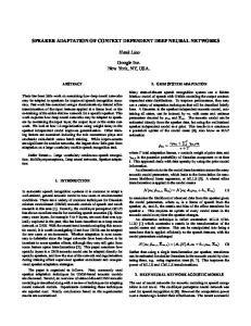
(a)

A1.2

A2.9

A3.7

(b)

A1

A2

A3

(c)

A

(d)

A

A

A

(e)

A.7

A.7

A.7

A.7

Fig. 1: Simple left-to-right HMM topologies. (a) A conventional 3state CD HMM. (b) A 3-state CI HMM (c) A one-state phone HMM (d) A tied-state CI phone model with minimum duration of 3. (e) A tied-state CD phone model with minimum duration of 4. ments given by forced-alignments with a 14,000 CD state DNN. The first LSTM has 126 softmax outputs corresponding to the context independent states of an HMM with 3 states per phone (mapping the CD labels of the alignment to the corresponding CI state). The second LSTM has 42 output states, one per phone, after mapping the alignments to the corresponding phone. These models are used for decoding with a simple HMM that has one state per phonetic unit (Figure 1(b) and (c) respectively). Results are shown in Table 1. We first observe that this phone model performs worse than the CI model. However, by changing the granularity of the acoustic model we have also changed the number of states per phone. This means that the minimum number of frames that must be expended in each phone has changed from 3 to 1, which by itself impacts recognition accuracy. By representing each phone with a 3-state HMM with tied distributions (Figure 1(d)), we can use the simple phone acoustic model but retain the minimum duration constraint, and achieve a similar WER, as shown on the last line of Table 1. Table 1: Word Error Rates of context-independent models. A 14000 state context dependent model trained with the same alignments achieves 10.7% WER. Model 126-state CI model 42-state phone model 42-state phone model with minimum duration 3

WER (%) 16.5 20.0 16.4

4. CONTEXT-DEPENDENT STATE CLUSTERING TREES We note that while modelling separate CI states instead of a single state per phone does not bring advantages, the context-independent model is significantly less accurate than a context-dependent 3-state model. Thus we argue that context dependency is still important and so we propose building context-dependent whole-phone units and training LSTM models to discriminate between them. We adapt a standard context-dependency clustering algorithm of Young et al. [9, 8] for the building of context-dependent phone models. The original algorithm takes force-aligned feature vectors,

collecting together all those vectors aligned to a particular CI state, and computing sufficient statistics on each subset with a particular phonetic context. Now, for each CI state we build a decision tree by binary divisive clustering. At each node of the tree we ask a set of binary phonetic questions about the context. Each such question splits the data in two, and from the sufficient statistics we can build a Gaussian model for each partition. The tree is extended by choosing the question which leads to the greatest likelihood gain. Tree building terminates when the likelihood gains are below a threshold, or when the leaves have too few observations. Here, we change the algorithm in three ways. First, instead of clustering with one tree per CI state, we build one tree per phone. Second, since we wish our acoustic states to model trajectories of acoustic features rather than piecewise stationary periods of acoustic features, instead of clustering all the frames assigned to each phone, we make a single representative feature vector for each example of that phone in the training set. A simple feature vector is constructed by concatenating the central frame from each state of the 3-state frame alignment (the alignment in this case comes from a previously-trained 3-state CI DNN system.) Third, following our previous work [8], we use the activations of the DNN’s penultimate layer as the feature representation used for clustering. The algorithm, with these 3 modifications, is applied as-is and results in 8367 context dependent phone models. For comparison, the baseline model obtained by clustering CI states using PLP features has 13522 CD states. The static CLG FSTs for the different C transducers are approximately the same size. By truncating the tree-building earlier, we can arrive at smaller inventories of context dependent phones and investigate the effect of different inventory sizes, as shown in Table 3. Throughout our experiments, we use the same state boundaries given by a CD-DNN model. Since the state inventories from truncated tree-building are nested, a simple many-to-one mapping can be applied to the original alignment labels to train with these smaller inventories. 4.1. Clustering on LSTM state Since we argue that the LSTM is modelling the acoustic trajectory throughout each phone, then it also seems natural that the LSTM state should be a good representation of that trajectory. Thus we repeat the same clustering algorithm using vectors of LSTM state from a previously trained two-layer LSTM model. Each phoneme in the training set is represented by the second LSTM layer’s state for the final frame of that phoneme, which is 800 dimensional. Clustering in this case results in 8491 CD phones.

5. DURATION MODELLING We observed in Section 3 that imposing a mimimum duration on the phone models improved WER, and that replicating states in a phone’s HMM was a simple way to achieve such a minimum duration model. We note that it is easier to apply such a duration model in a whole-phone HMM since the aggregate duration is less noisy and subject to quantization than the three separate discrete duration distributions. An effect equivalent to repeating states can be achieved more efficiently by explicitly handling duration in the decoder. In practice we can supply a minimum duration for each model independently. While there is an extensive literature on duration modelling in HMMs for speech and handwriting, our baseline system effectively has no duration model (self and next transition probabilities are both 0.5 for all states, so all paths result in the same product of transition probabilties). A simple way to estimate a minimum duration model is based on the duration histogram observed on the training set. For simplicity we took the original alignments used for the training, and computed duration histograms for the CD-phone models at each level of the clustering hierarchy. Figure 2 shows the cumulative histograms for the phone models. Every phone has a duration of 3 or more states because the alignment was done with a 3-state HMM, but it can be seen that the observed distribution is quite different for different phones. Thresholding the cumulative probability (we found a threshold of 10% of the probability mass to give the best results in initial tests), we arrive at a minimum duration for each CD-state (shown in Figure 1(e)), though for the special case of silence we relax to a 3-state minimum duration. Table 2 shows the effect of different duration models when testing the 8397-state CD phone LSTM acoustic model. It can again be seen that imposing a minimum duration is essential for good performance, with the best performance when every model has duration 4. Setting a minimum duration per phone gives better results, but the best performance is found when the minimum duration is chosen separately for each CD-phone model. Table 2: Word error rates for CD phone models with different minimum-duration models, using the 8397-CD-phone LSTM acoustic model. Duration 1 state 3 state 4 state 5 state Per-phone Per-CD phone

WER 12.3 10.4 10.2 10.3 10.1 10.0

4.2. Clustering right context It should be noted that using the connectionist temporal classification (CTC) algorithm [10] with bidirectional LSTMs has shown good results on whole-phone models [11, 12] without the need for contextdependent modelling. We argue that the bidirectionality provides the model with evidence for the acoustic context and thus the LSTM model itself is modelling the distribution given the context, in the same way that choosing a context-dependent unit on the basis of the search graph conditions the distribution on the context. Since we have a unidirectional model which is aware of the left, but not right, context, we investigated the effect of clustering only based on the right phonetic context. For these experiments, we again used the LSTM state features, and clustering resulted in 1120 CD phone units.

Table 3 compares the three different methods of clustering CDphones (based on DNN-activation, LSTM state or LSTM-state with right-context only) with the standard CD-state inventory. In each case we compare different sizes of state inventory. We first observe that the whole-phone CD models with 8367/8491 states perform as well as the conventional CD state model with 13522 states (and better than the CD state model with 8000 states). For smaller state inventories the performance is roughly comparable. We observe that the two feature types we have used for CD phone tree building result in similar performance. It appears not to be sufficient to only cluster on the right context, although the state inventory is small (1120) it represents 70% of the possible rightclustered diphone units possible.

Table 3: Clustering on LSTM state vs acoustic features. In each CD phone evaluation we use the per-CD-phone minimum duration model. States 500 1120 2000 ~8300 13522

Acoustic features 12.0 – 11.6 10.0 –

CD phones LSTM State 12.4 – 11.3 10.0 –

Right only 12.1 11.7 – – –

CD states 12.1 – 11.0 10.5 10.1

6. CONCLUSIONS AND FURTHER WORK

0.7

D OI eI oU s sil t

0.6 0.5 0.4 0.3 0.2 0.1 0.0

4

6

8

10

12

14

4

6

8

10

12

14

0.7 0.6 0.5 0.4 0.3 0.2 0.1 0.0

Fig. 2: Cumulative duration histograms for selected models measured on the training set alignments. The dashed line shows the 10% threshold used here to determine a minimum duration threshold. Top: whole-phone durations. Bottom: The 21 different CD variants of the “OI” phone from the 8491-CD inventory show considerable diversity.

In this paper we have shown that the conventional multi-state phone model used with GMMs and DNNs is not necessary with LSTM acoustic models. We have shown that, with a simple duration model, a context-dependent triphone model can equal the performance of a 3-state context-dependent triphone model. This reduces the number of states that must be modelled and consequently the number of parameters and acoustic model computational burden. Since we have shown the importance of even a simple minimum duration model, we plan to investigate stronger modelling of the CDphone duration distributions. The models described here were all trained on the same DNN-based alignment and one or more iterations of realignment and retraining of both the LSTM and the duration model may result in a more consistent and thus more accurate model. Further, we have recently [13] shown improvements in WER (around 10% relative) from sequence training [14] of LSTM acoustic models. We have still to investigate whether such gains can also be demonstrated for these CD phone models. Finally, we plan to investigate whether these context dependent models can be used in conjunction with the CTC algorithm that has hitherto only been used with context independent whole-phone models, but which can nevertheless achieve word error rates close to that of conventional CD state models [12].

7. REFERENCES [1] G. Hinton, L. Deng, D. Yu, G.E. Dahl, Mohamed A., N. Jaitly, A. Senior, V. Vanhoucke, P. Nguyen, T.N. Sainath, and B. Kingsbury, “Deep neural networks for acoustic modeling in speech recognition,” IEEE Signal Processing Magazine, vol. 29, pp. 82–97, November 2012. [2] A. Graves, N. Jaitly, and A.-R. Mohamed, “Hybrid speech recognition with deep bidirectional LSTM,” in Automatic Speech Recognition and Understanding (ASRU), IEEE Workshop on. IEEE, 2013, pp. 273–278. [3] H. Sak, A. Senior, and F. Beaufays, “Long Short-Term Memory Based Recurrent Neural Network Architectures for Large Vocabulary Speech Recognition,” ArXiv e-prints, Feb. 2014. [4] H. Sak, A. Senior, and F. Beaufays, “Long Short-Term Memory Based Recurrent Neural Network Architectures for Large Vocabulary Speech Recognition,” in Interspeech, 2014. [5] S. Hochreiter and J. Schmidhuber, “Long short-term memory,” Neural Computation, vol. 9, no. 8, pp. 1735–1780, Nov. 1997. [6] F. A. Gers, J. Schmidhuber, and F. Cummins, “Learning to forget: Continual prediction with LSTM,” Neural Computation, vol. 12, no. 10, pp. 2451–2471, 2000. [7] H. Bourlard and N. Morgan, Connectionist speech recognition, Kluwer Academic Publishers, 1994. [8] A. Senior, G. Heigold, M. Bacchiani, and H. Liao, “GMM-free DNN training,” in Proc. ICASSP, 2014. [9] S. Young, J. Odell, and P. Woodland, “Tree-based state tying for high accuracy acoustic modelling,” in Proc. ARPA Human Language Technology Workshop, 1994. [10] A. Graves, Supervised Sequence Labelling with Recurrent Neural Networks, Springer, 2012. [11] A. Graves, A. Mohamed, and G. Hinton, “Speech recognition with deep recurrent neural networks,” in Proc. ICASSP, 2013. [12] H. Sak, A. Senior, K. Rao, O. Irsoy, A. Graves, F. Beaufays, and J. Schalkwyk, “Learning acoustic frame labeling for speech recognition with recurrent neural networks,” in submitted to ICASSP, 2015. [13] H. Sak, O. Vinyals, G. Heigold, A. Senior, E. McDermott, R. Monga, and M. Mao, “Sequence discriminative distributed training of long short-term memory recurrent neural networks,” in Interspeech, 2014. [14] B. Kingsbury, “Lattice-based optimization of sequence classification criteria for neural-network acoustic modeling,” in Proc. ICASSP, Taipei, Taiwan, Apr. 2009, pp. 3761–3764.