Compartmental Fluid-Flow Modelling in Packet Switched Networks with Hop-by-Hop Control

Vincent Guffens Membres du jury: Georges Bastin (Promoteur) Benoˆıt Macq Hugues Mounier Olivier Bonaventure Thierry Divoux Vincent Wertz (Pr´esident)

ii

Acknowledgements

Je remercie mon promoteur, le Professeur G. Bastin, pour son encadrement efficace et ses critiques constructives qui m’ont permis de mener `a bien ce travail de th`ese. Je remercie ´egalement Hugues Mounier pour son accueil ainsi que pour son encadrement scientifique durant mon s´ejour `a l’Ecole des Mines de Paris organis´e dans le cadre du programme Control Training Site ainsi que le Professeur Benoˆıt Macq pour ses encouragements initiaux. Merci aux membres du jury pour leur relecture du manuscrit ainsi que pour la discussion fructueuse lors de la d´efense priv´ee qui a activement contribu´e `a la version finale de ce document. Enfin, je remercie les promoteurs du PAI et du CTS pour leur soutien financier.

iii

Preamble Packet switched networks offer a particularly challenging research subject to the control community: The dynamics of a network buffer, their simplest component, are nonlinear and exhibit a saturation effect that cannot be neglected. In many practical cases, networks are made up of the interconnection of a large number of such basic elements. This gives rise to high dimensional nonlinear systems for which few general results exist today in the literature. Furthermore, these physical interconnections that may sometimes span a very long distance induce a transmission delay and the queues in intermediary nodes induce a buffering delay. Transmission delays are mathematically equivalent to partial differential equations and are often difficult to analyse. They may also cause radical changes in the qualitative behaviour of a system and increase the difficulty of designing good controllers. Buffering delays are state dependent and their analysis is not equivalent to the study of pure transmission delays. The asynchronous nature of the per-packet transmission also poses a difficult modelling problem : packet switched networks do not fit in either a discrete time system model where events occur at regular time intervals nor do they fit into a continuous time system where the flow of information is defined for any arbitrarily small time interval. Finding a model able to both take into account as much of this complexity as possible while being simple enough to be analysed mathematically and used for control purposes is the first objective of this thesis. Our model is constructed in Chapters 2, 4 and 5. Chapter 2 introduces the core element of the model, the modelling of a first in first out (FIFO) buffer. The modelling approach lies into the fluid flow modelling paradigm. That is to say that the traffic flow is viewed as a continuous stream, just like a flow of water between recipients. This modelling approach can be justified by considering an averaged flow of packets over a suitable time interval. An alternative justification is also given in Chap. 2 using a queueing theory perspective. In chapters 4 and 5, these simple elements are interconnected to fit a given network topology. This gives rise to a set of nonlinear ordinary differential equations. Another important modelling decision has been to construct a model with a C 1 vector field. This latter decision may also be justified using queueing theory arguments as described in chap. 2. Because our model is based on a mass conservation principle around each buffer, the dynamical system that is obtained turns out to be compartmental. Chapter 1 summarises some important known results about this class of systems which can be readily applied to obtain global results

iv

for our models. The second objective of this thesis is to design a feedback control law able to globally stabilise the derived system. This is in contrast with most results available in the literature which are usually concerned with local stability as recalled in Chapter 1. In order to fulfil that goal, Chapter 4 also introduces a fluid flow model of a well known network element, the so-called “token-leaky bucket”. The token leaky bucket can be seen as a tool that achieves a rate control using tokens. These token-leaky buckets are connected in feedback from one node to another which results in a “hop-by-hop” control strategy. Using these tokenleaky buckets is important as it allows an easy implementation of our control law. In Chapter 5 a model suitable for the global description of a general topology with hop-by-hop control is derived. However, in order to be able to guarantee the global stabilisation of the system, a specific router architecture has to be considered. This is one of the drawbacks of our approach, this restriction being needed only to apply available theoretical results and being not justified by any physical considerations. The derived model may nevertheless still be used for both fluid-flow simulations and obtaining provable mathematical properties such as the boundedness of packet queue length for more general situations. Throughout the text some simulation results obtained by integration of the fluid-flow model are presented. Whenever relevant, these simulation results are compared with experimental measurements obtained on a network of virtual Linux machines. Chapter 6 describes the implementation of the proposed hop-by-hop control law in Linux as well as the implementation of the specific router architecture used in Chap. 5 with omnet++. These experimental results demonstrate the feasibility of our approach and also validate the fluid-flow models. The availability of a general network model allows for a rigorous mathematical analysis of the system and is therefore very useful to apply the control theory tools. Some reference papers cited in Chapter 1 use feedback linearisation, Smith’s predictors and, of course, linearised system analysis. Besides system analysis, such models also allow to apply optimisation tools. Although applying optimisation theories on large scale nonlinear dynamical systems such as those presented in this work is rather prospective, Chapter 3 presents an optimal control strategy of a single network buffer using Pontryagin’s principle. This yields a non trivial and non intuitive heuristic control which only requires simple network measurements. As described in Chapter 3, these measurements are really what one could cal “fluid-flow” measurements and are very different from the data that can usually be collected on a real system such as the Linux kernel. This alternative way of measuring some variables on

v

an intrinsically discrete event asynchronous system as a result of a fluid flow analysis might well give hope for future results using our modelling approach. The hop-by-hop strategy mentioned above is based on the conservation of packets between two neighbouring nodes in a network. This is also the root idea behind popular end-to-end control strategies which allow new packets to be sent in the network only when a packet arrival has been acknowledged by its destination. Compartmental systems are very well suited for the description of such dynamics. Therefore, in Chapter 7, a generalised controller that is based on the conservation of the total system mass is presented. Furthermore, extra dynamics of the end-to-end controller might be seen as the perturbation of a system with a constant total mass. Using singular perturbation analysis the global dynamics of such a perturbed system can therefore be analysed. This means that the end-to-end control law is analysed taking into account the queueing delay which is modelled by way of a compartmental network of queues. Chapter 7 is concluded with the presentation of a new end-to-end control law which seems particularly well suited for interacting with a hop-by-hop controller. However, it is shown that the dynamics of such a system might be quite complicated and that its analysis is very challenging. This message is, however, applicable to this entire thesis. If global results may be obtained using known compartmental system results, they are also limited by them. Most results related to end-to-end control, notably the famous Transport Control Protocol (TCP) do not deal with this mass conservation and concentrate on other important problems such as the fairness of the resulting rate allocation. It might indeed seem rather obvious that a system which merely ensures the conservation of its total mass is rather trivial. In fact, compartmental systems have strong structural constraints and it is therefore quite natural to think that their dynamical behaviour is also strongly constrained. Jacquez and Simon report that Bellman, in one of his 1970 paper dealing with pharmacokinetics, conjectured that nonlinear autonomous closed compartmental systems had a unique globally stable equilibrium point. However, the same authors have shown in 1993 that these systems may in fact show the full range of possible behaviours of systems of ordinary differential equations ! In his famous 1988 paper describing the behaviour of the TCP control, Jacobson states that the TCP control relies on the conservation of packets around each source-destination pair; in a footnote it is stated that these loops are Lyapounov functions for the controlled system and that they therefore guarantees the stability of said system. However, in a compartmental model, these loops are not Lyapounov functions but are first integrals

vi

for the system, which does not guarantee any stabilisation. As it is quite likely that the stability referred to in the Jacobson’s paper only refers to the non-attractivity of the origin or the so-called congestion collapse, our approach therefore sheds new light on network stability analysis. These arguments are discussed more in depth in Chapter 7. Finally, the pictures that appear at the beginning of each chapter are taken from the 1927 Fritz Lang movie “Metropolis”. This sciencefiction story presents a heavily industrialised underworld dominated by a powerful society living on the surface. It is surprising how this old representation of the industrialised future resembles our globally internetworked society breathing through its vital interconnections. In 80 years of time, it shows tremendous technological advances and surprising unchanged patterns.

vii

Publication list Journal articles 1. G. Bastin, V. Guffens, Congestion control in compartmental network systems, accepted for publication in Systems and Control Letters. ´ 2. V. Guffens, M. Hilgers, Ed., Pour le libre, Dossier de La revue Nouvelle, Num´ero 6, Juin 2005.

Conference proceedings 1. V. Guffens, G. Bastin, H. Mounier, Fluid flow network modeling for hop-by-hop feedback control design and analysis, In CD-Rom proceedings Internetworking 2003, San Jose, CA, USA, June 22-24, 2003. 2. V. Guffens, G.Bastin, H. Mounier, Using token leaky buckets for congestion feedback control in packet switched networks with guaranteed boundedness of buffer queues, Paper 175 in CD-Rom Proceedings European Control Conference ECC 03, Cambridge (UK), September 2003. 3. V. Guffens, G. Bastin, H. Mounier, Utilisation de seaux perc´es a jetons pour le controle de type ”proche-en-proche” dans les reseaux de communication, Article 168 CD-Rom, Conf´erence Internationale d’Automatique CIFA 2004, Douz, Tunisie, 22-24 Novembre 2004. 4. V. Guffens, G. Bastin, Running virtualized native drivers in User Mode Linux,in Proc. of 2005 USENIX Annual Technical Conference, p. 33-40, Anaheim, USA, April 10-15 2005. 5. V. Guffens, G. Bastin, Optimal Adaptive Feedback Control of a Network Buffer, in Proc. of American Control Conference ACC2005, Portland, USA, June 8-10 2005, pp. 1835-1840. (Best paper in session)

Contents

1 Background 1.1 An introduction to hop-by-hop flow control 1.1.1 The need for congestion control . . . 1.1.2 End-to-End flow control . . . . . . . 1.1.3 Hop-by-Hop flow control . . . . . . . 1.1.4 Hop-by-Hop and End-to-End control 1.1.5 A review of selected papers . . . . . 1.2 An introduction to compartmental systems 1.2.1 What is a compartmental system . . 1.2.2 Properties of compartmental systems 1.3 Conclusion . . . . . . . . . . . . . . . . . .

. . . . . . . . . .

. . . . . . . . . .

. . . . . . . . . .

. . . . . . . . . .

. . . . . . . . . .

. . . . . . . . . .

. . . . . . . . . .

2 Fluid flow modelling of a FIFO buffer 2.1 Physical model . . . . . . . . . . . . . . . . . . . . . . . 2.1.1 Fluid flow model of the buffer-server . . . . . . . 2.1.2 Modelling of the processing rate . . . . . . . . . 2.1.3 Modelling of the Linux switching architecture . . 2.1.4 Modelling of irreversible overflows . . . . . . . . 2.1.5 Router architecture . . . . . . . . . . . . . . . . . 2.2 Queueing theory perspective . . . . . . . . . . . . . . . . 2.2.1 Illustration . . . . . . . . . . . . . . . . . . . . . 2.2.2 Relationship with other processing rate functions 2.3 (Min,+) theory perspective . . . . . . . . . . . . . . . . 2.3.1 An equivalent (Min,+) system . . . . . . . . . . 2.3.2 Relationship with the processing rate (2.2) . . . 2.4 Conclusion . . . . . . . . . . . . . . . . . . . . . . . . . ix

. . . . . . . . . .

1 1 1 2 4 5 6 18 18 19 22

. . . . . . . . . . . . .

25 25 26 27 28 30 32 33 34 35 37 38 41 43

x

3 Application: Optimal fluid flow control of a 3.1 Fluid flow model with tail-drop policy . . . 3.1.1 Tail-drop policy . . . . . . . . . . . . 3.2 Optimal control . . . . . . . . . . . . . . . . 3.2.1 Minimisation of the Hamiltonian . . 3.2.2 Boundary conditions . . . . . . . . . 3.2.3 Example . . . . . . . . . . . . . . . . 3.2.4 Other optimum scenari . . . . . . . 3.2.5 Integration method . . . . . . . . . . 3.3 Implementation of the optimal control . . . 3.3.1 Fluid flow measures . . . . . . . . . 3.3.2 On-line model identification . . . . . 3.3.3 Adaptive threshold . . . . . . . . . . 3.4 Simulation results . . . . . . . . . . . . . . 3.5 Simulation results with a real network trace 3.6 Scope of the result . . . . . . . . . . . . . . 3.7 Conclusion . . . . . . . . . . . . . . . . . .

CONTENTS

FIFO buffer . . . . . . . . . . . . . . . . . . . . . . . . . . . . . . . . . . . . . . . . . . . . . . . . . . . . . . . . . . . . . . . . . . . . . . . . . . . . . . . . . . . . . . . . . . . . . . . . . . . . . . . . . . . . . . . . . . . . . . . . . . . . . . . .

4 A chain of routers under Hop-by-Hop control 4.1 A fluid flow model of the token leaky buffer . . . . . . . 4.1.1 Burstiness Constraint . . . . . . . . . . . . . . . 4.2 A token leaky buffer with feedback . . . . . . . . . . . . 4.2.1 Property . . . . . . . . . . . . . . . . . . . . . . . 4.2.2 Burstiness constraint . . . . . . . . . . . . . . . . 4.2.3 Credit-based and rate-based flow control . . . . . 4.2.4 Interconnection with delay . . . . . . . . . . . . 4.2.5 Practical implementation of the feedback loop . . 4.2.6 Links with large bandwidth delay products . . . 4.2.7 Experimental validation of the token leaky buffer with feedback . . . . . . . . . . . . . . . . . . . . 4.3 Compartmental modelling of a chain of router with HBH control . . . . . . . . . . . . . . . . . . . . . . . . . . . . 4.3.1 Compartmental model . . . . . . . . . . . . . . . 4.3.2 Properties . . . . . . . . . . . . . . . . . . . . . . 4.3.3 Proof . . . . . . . . . . . . . . . . . . . . . . . . 4.3.4 I/S characteristic . . . . . . . . . . . . . . . . . . 4.4 Experimental validation . . . . . . . . . . . . . . . . . . 4.5 Limit-cycles . . . . . . . . . . . . . . . . . . . . . . . . . 4.6 Relationship with (min,+) theory . . . . . . . . . . . . . 4.6.1 Proof . . . . . . . . . . . . . . . . . . . . . . . . 4.7 Conclusion . . . . . . . . . . . . . . . . . . . . . . . . .

. . . . . . . . .

45 45 46 47 48 50 50 51 55 56 57 57 59 59 62 63 65 69 69 70 71 72 72 72 73 74 75

. 75 . . . . . . . . . .

78 78 79 80 82 83 86 90 91 96

CONTENTS

xi

5 Compartmental modelling of communication networks 97 5.1 Modelling of a general topology . . . . . . . . . . . . . . . 97 5.2 Hop-by-hop congestion control . . . . . . . . . . . . . . . 101 5.2.1 Implementation with token buckets . . . . . . . . . 101 5.2.2 Case study : Implementation with a crossbar switching architecture . . . . . . . . . . . . . . . . . . . . 102 5.2.3 Experimental validation with a discrete event simulator . . . . . . . . . . . . . . . . . . . . . . . . . 103 5.2.4 Performance issues . . . . . . . . . . . . . . . . . . 105 5.3 Application: Control of a single rate multicast flow . . . . 108 5.3.1 A general fluid flow model . . . . . . . . . . . . . . 109 5.3.2 Properties . . . . . . . . . . . . . . . . . . . . . . . 109 5.3.3 Simulations and experimental results . . . . . . . . 110 5.4 Conclusion . . . . . . . . . . . . . . . . . . . . . . . . . . 111 6 Implementation of the HBH strategy 6.1 The path of a packet in the Linux kernel . . . . . . . . . 6.2 Implementation of the token leaky buffer with feedback 6.3 Isolation of the controlled flow . . . . . . . . . . . . . . 6.4 Implementation of the cross-bar switching architecture . 6.4.1 Structure of the input interfaces . . . . . . . . . 6.4.2 Fairness enhancement . . . . . . . . . . . . . . . 6.5 Conclusion . . . . . . . . . . . . . . . . . . . . . . . . .

115 . 115 . 117 . 120 . 121 . 121 . 122 . 123

7 End-to-end and Hop-by-hop control 125 7.1 E2E congestion control: a mass conservation point of view 125 7.1.1 Numerical example . . . . . . . . . . . . . . . . . . 131 7.2 Singular perturbation analysis of an AIMD algorithm . . 133 7.2.1 Model of the additive increase, multiplicative decrease mechanism . . . . . . . . . . . . . . . . . . . 134 7.2.2 Global network model with end-to-end congestion control . . . . . . . . . . . . . . . . . . . . . . . . . 136 7.2.3 Singular perturbation analysis . . . . . . . . . . . 137 7.3 Combining End-to-end and Hop-by-hop control . . . . . . 140 7.3.1 Limitation of hop-by-hop flow control . . . . . . . 140 7.3.2 HBH and E2E control with a rate-based marking scheme . . . . . . . . . . . . . . . . . . . . . . . . . 142 7.4 Related work . . . . . . . . . . . . . . . . . . . . . . . . . 148 7.5 Conclusion . . . . . . . . . . . . . . . . . . . . . . . . . . 150

xii

CONTENTS

8 Conclusions and perspective 151 8.1 Conclusion . . . . . . . . . . . . . . . . . . . . . . . . . . 151 8.2 Perspective . . . . . . . . . . . . . . . . . . . . . . . . . . 153 References A A brief introduction to (min,+) theory and culus A.1 Example . . . . . . . . . . . . . . . . . . . . A.2 Mathematical structure . . . . . . . . . . . A.3 Wide sense increasing and good functions . A.4 (min,+) convolution . . . . . . . . . . . . . A.5 Conclusion . . . . . . . . . . . . . . . . . .

155 network cal163 . . . . . . . . 163 . . . . . . . . 164 . . . . . . . . 165 . . . . . . . . 166 . . . . . . . . 166

B User Mode Linux as a network simulator 167 B.1 User Mode Linux architecture . . . . . . . . . . . . . . . . 167 B.2 User Mode Linux as a network simulator . . . . . . . . . . 169 B.3 Conclusion . . . . . . . . . . . . . . . . . . . . . . . . . . 171

Chapter 1

Background 1.1

An introduction to hop-by-hop flow control

Hop-by-hop flow control refers to congestion control techniques where each node receives information from its directly connected neighbours. Intermediate nodes use this information to take decision on the fate of forwarded packets (drop, forward, delay the packets. . .). This is in contrast with end-to-end congestion control techniques where information about the congestion of the network is sent back to the sources connected to that network which may then take actions to reduce the detected congestion.

1.1.1

The need for congestion control

Early communication networks such as the public telephone networks of the 1950’s where circuit oriented. In these networks, a communication channel is established between communicating peers and the resources needed for the communication are reserved before the communication takes place. Therefore, the problem of congestion, that we loosely define (see below for a more formal definition) as a a temporary overflow of the network capacity, can not happen as sufficient resources have been statically reserved. The drawback of such an approach is however that the available resources are used inefficiently. Unused reserved resources are indeed lost and cannot be used for other connections. To achieve a better resource utilisation, available resources should therefore be shared between multi1

2

Chapter 1. Background

ple connections. This technique, referred to as statistical multiplexing is the core idea behind packet switched networks where packets belonging to different connections share common buffers in intermediate nodes. Clearly this new situation leads to points of traffic aggregation and might therefore create bottlenecks in the network. A common definition for congestion, closely related to this idea of bottleneck can be found in Keshav [54] : A network is said to be congested from the perspective of user i if the utility of i decreases due to an increase in network load. This definition uses well known terms borrowed from the economic science literature such as the “user utility” which captures the idea of quality of service as perceived by a user. The first control congestion schemes started to appear in the literature in the early 1980’s (Gerla and Kleinrock [30], Pouzin [93]). In the end of the 1980’s, the number of data networks such as ARPANET had grown and optical fibres were available. Large bandwidth delay products typical of long distance connections with fibres (Kleinrock [57]) worsened the congestion problem. Congestion avoidance and control techniques able to tackle this problem were then published such as the famous congestion avoidance and control paper from Jacobson in 1988 (Jacobson [43]) which introduces TCP. Another important protocol is known as Decbit and was presented in 1987 in [95] and published in [96]. This protocol introduces the use of a one bit feedback scheme with additive increase multiplicative decrease policy. It later inspired work such as Explicit Congestion Notification (TCPECN) and ATM 1-bit feedback scheme. Given the importance of this class of protocols, a brief introduction on end-to-end control is presented in the next section. Readers interested in the historical perspectives of congestion control may refer to Keshav [54].

1.1.2

End-to-End flow control

End-to-end (E2E) flow control schemes are usually implemented in protocols mapping to the transport layer (layer 4) of the reference Open System Interconnection (OSI) model. Other important functionalities implemented at that layer are : multiplexing, virtual circuit management, error checking and recovering [23, p6] In this family of protocols, one can find, for instance : NETBLT [101], DECbit and of course TCP [100]. TCP is certainly the most

1.1. An introduction to hop-by-hop flow control

3

widely used transport protocol. The two others are cited here for historical reasons. The principle of these protocols is that the sender maintains a window of packets in transit toward the destination. Each packet is numbered so that the destination may acknowledge its reception and the sender may then slide the window to allow new packets to be sent. When the sender detects a congestion in the path toward the destination, the window size can be reduced in an effort to relieve the congestion. The congestion control problem is therefore translated to a window management problem. Note that the sliding window mechanism is a flow control mechanism while the management of the window’s size is the congestion control mechanism. These two mechanisms, although tightly linked, are two different concepts. DECbit and TCP use a system known as “additive increase, multiplicative decrease” for the window’s management: the size of the window increases by a fixed amount with each acknowledgement from the receiver while it is divided by two when the sender detects a congestion condition. The congestion indication is said to be implicit in the sense that the sender derives the information from events resulting from the congestion. Such an event is typically the expiration of a timer while waiting for some acknowledgements from the receiver. NETBLT uses a different flow control method: rate control. A rate is negotiated between the sender an the receiver and the receiver uses timer rather than acknowledgements from the receiver to maintain the negotiated rate. The rate can be re-negotiated according to observed performance. Some other congestion control mechanisms may also be found at the layer 2 of the OSI model in data-link protocols such as FRAME-RELAY [23, chap 10] or ATM [23, chap 20]. In these protocols, the network may explicitly set a Forward-Explicit Congestion Notification bit in the datalink header to inform the receiver that this packet experienced congestion. Similarly, a Backward-Explicit Congestion Notification bit may be set by intermediate device in packets travelling in the opposite direction to inform the sender of the existence of congestion on the link. More recently, an explicit congestion notification scheme (ECN) has been proposed for the TCP/IP protocol suite [99]. With the addition of ECN, intermediate routers can set the Congestion Experienced (CE) bit in the IP header. Therefore, actions taken by sources to reduce the congestion can be taken before any packet loss is experienced.

4

Chapter 1. Background

Figure 1.1: End-to-end congestion scheme compared to hop-by-hop control.

1.1.3

Hop-by-Hop flow control

Although successful solutions to congestion problems in packet switched networks have been end-to-end congestion control schemes, an alternative methodology has been known and studied since the problem has been stated. The principle of this alternative method, known as “hopby-hop” (HBH) is illustrated in Fig. 1.1 and compared to end-to-end control. In hop-by-hop controlled networks, each node broadcasts congestion information to its directly connected neighbours which can immediately take actions to reduce the congestion and, in turn, broadcast their congestion state to their upstream neighbours. Descriptions of HBH flow control techniques can be found in some classical networking books such as in Bertsekas and Gallagher [8, chap 6] which describes a node-by-node windows flow control for virtual circuits (VC). In this description, each VC, in each node, is controlled by a separate window. The size of the window, denoted W [in packets] is typically small, of the order of 2. The interaction of successive windows along the path produces a back-pressure effect as buffers fill up one after the others in nodes upstream a congested link. If there are n such nodes, the number of packets waiting in the network is nW which is therefore equivalent to an end-to-end control with a window of nW packets. However, the memory required in each router in the HBH case is much smaller as the waiting packets are uniformly distributed along the congested path. However, for high speed or long delay links, the size W of the corresponding window must be increased in order to operate the link at its maximum capacity. This might therefore, in heterogeneous networks, induce some fairness problems if different links are controlled by windows of different sizes.

1.1. An introduction to hop-by-hop flow control

5

A network using such a flow control mechanism, called Tymnet and initially called Tymshare, began operation in 1966. The fairness of the HBH scheme was enhanced by servicing the VC via a round-robin scheme. Flow control permits were encapsulated into dataframe for transmission to upstream neighbours. Tymnet was shut down in March 2003. In another classical book by Tanenbaum [111, chap 5.3], a description of a HBH method is given under the name “hop-by-hop choke packet” : Each router monitors its resource utilisation, if resource utilisation goes above a threshold, new arriving packets trigger the sending of a choke packet to the source, including the destination of the newly arriving packet. The source is then required to decrease its sending rate toward the destination∗ . In high-speed networks, a lot of data may have been sent before the source receives the choke packet. A quick relief at the point of congestion is obtained if the choke packet takes effect at every node it passes through, that is to say, by using HBH techniques. A mathematical analysis of such a technique can be found in Mishra and Kanakia [78] as detailed in the following section 1.1.5.

1.1.4

Hop-by-Hop and End-to-End control

Obviously, HBH and E2E control strategies are not incompatible and they may therefore be used simultaneously. One such way of combining these two approaches is to use a HBH control mechanism at the layer 2 of the OSI model while using an E2E control mechanism at the layer 4. As mentioned at the end of this chapter, pause frame are used in 802.3 fullduplex gigabit networks, which, in conjunction with TCP, is an example of such a combination. The problem of choosing between a rate-based, credit-based, HBH, E2E or both HBH and E2E has emerged during the discussion preceding the adoption of the ATM standard. In [47], the various reasons and motivations for accepting one technique or another are presented. The figure 1.2, found in [47], shows the complementarity of the two approaches with respect to the time scale at which they apply. It can be seen that link-by-link feedback (HBH) is presented as suitable for shorter time interval while end-to-end feedback is suitable for a longer congestion duration. Credit based HBH techniques where then proposed with a per virtual chanel (VC) bucket. This proposal was discarded as being not scalable with respect to the number of VC’s. ∗ This approach has been implemented in the IP protocol suite as ICMP source quench message. It however suffers from security problems and has now been deprecated.

6

Chapter 1. Background

congestion duration

LONG

SHORT

congestion mechanism Capacity planning and network design Connection admission control Dynamic routing Dynamic compression End−to−end feedback Link−by−link feedback Buffering

Figure 1.2: Congestion techniques for various congestion durations (from [47]).

Another proposal, which combines a per-link HBH scheme with a 1-bit E2E rate-based congestion control ([47, Sec 6.5]) was also discarded. A rate-based version of the DECbit scheme was finally adopted ([47, Sec. 8]). As discussed later in this chapter, some simulations have shown ([89, 88]) that using HBH with TCP has the potential to improve the TCP perfomances. However, to the best of our knowledge, their exists no global theoretical analysis able to describe the performance of a HBH control combined with E2E control for an arbitrary topology.

1.1.5

A review of selected papers

Although it is clear that the literature in HBH control does not compete in quantity with end-to-end control, it is also clear that HBH control is a recurrent subject : HBH techniques have been proposed in response to many networking challenges such as flow control, multicast delivery, TCP performance . . . They have been proposed for virtual path flow control in ATM networks and some variants exist under the form of XON-XOFF control in gigabit networks. We now review some of the articles that present and analyse these concepts with a particular emphasis on the paper from Mishra and Kanakia [78] given its importance in the HBH literature. We also divide the presentation in two broad categories “rate based” and “credit based” techniques, according to a classification that also exists in endto-end literature. On Rate-based HBH flow control In [78] (see also [77]), Mishra and Kanakia analyse a HBH rate-based congestion control scheme. They provide an asymptotic stability analysis and some simulations as well as a mechanism to use newly available bandwidth effectively. The variance of the queue occupation is also studied. The topology under investigation is limited to a chain of routers.

1.1. An introduction to hop-by-hop flow control switch i µ ki

x ik

7

switch i+1 µi+1 k

x i+1 k

µi+2 k

Figure 1.3: Illustration of the fluid model proposed in [78].

Fluid flow model The proposed fluid flow model gives the queue occupancy xik of the ith buffer at discrete time steps k (see Fig. 1.3). The idea is to sample the system at regular time interval, every d seconds. Feedback packets, as we shall see later, are also sent every d seconds so that the sampling instants correspond to the emission of such a feedback packet. Due to propagation delays, j feedback packets are sent during the round trip time between two adjacent switches as illustrated in Fig. 1.4. The buffer occupancy may be calculated as follows : xik = xik−1 + d(µik−1 − µi+1 k−1 )

(1.1)

which simply states that the number of packets in the ith buffer at time k is the number of packets already present at time k − 1 plus the difference between the number of packets that have entered the queue and those that have left the queue during the last sampling interval. In order to ensure the positivity of the queue size, the model becomes : xik = max{xik−1 + d(µik−1 − µi+1 k−1 ), 0} and to take into account the maximum buffering capacity of the queue, denoted Bmax , the model is finally rewritten as :  xik = min max{xik−1 + d(µik−1 − µi+1 (1.2) k−1 ), 0}, Bmax This model is then used to derive a rate-based control law suitable for driving the buffer occupancy in each switch toward a predetermined setpoint. Prediction control mechanism A switch computes the target sending rate to drive the future state of the system at the downstream switch to setpoint x∗ . At switch i − 1, the target rate is computed as : λik = µi+1 + k

x∗ − xik g d

(1.3)

with g, a gain parameter. The choice of this particular target rate is rather obvious. Replacing µik−1 in eq. (1.1) with g = 1 by this expression

8

Chapter 1. Background

i xk i x k+1

j=4 d RTT

i

x k+4 switch i

switch i+1

Figure 1.4: Timing diagram for [78]: the flow of time is represented vertically, from top to bottom. Four feedback periods (j = 4) elapse during the round-trip-time (RTT) between two adjacent switches.

yields xik = x∗ which means that if the switch i is fed at the rate λik the target setpoint is reached. Of course, the value of xik and µi+1 are not k known at switch i − 1 at time k. Therefore, the predicted values x ˆik i+1 and µ ˆk are used instead using a first order auto-regressive filter with parameter α. µ ˆi+1 k−j

= αµi+1 µi+1 k−j−1 + (1 − α)ˆ k−j−1

x ˆik = xik−j + d

k−1 X

(µip − µ ˆi+1 p )

(1.4) (1.5)

p=k−j

. Analysis with white noise In this analysis, the bottleneck service rate is approximated by a constant value M plus white noise to take into account the cross-traffic. This analysis gives insight into the choice of parameters to provide good steady state performance. The analysis is realised in a chain topology with the last link being the bottleneck. The buffer output rates are therefore :  M + k if node i is the bottleneck i+1 µk = λi+1 otherwise k with k a zero-mean white noise sequence with a variance of σ 2 . The system (1.2)-(1.5) being non-linear, a linearised version around the equilibrium point x = x∗ , µ = M is considered instead. It is then shown, using standard results from linear algebra, that the system (1.2)-(1.5) is locally stable for the following choice of parameters : 0
−1<α<1

1.1. An introduction to hop-by-hop flow control

9

The variance of the queue occupancy is studied numerically as analytical results were found to be intractable. It is shown that for low values of α, an increasing value of g reduces the variance and that the converse is true for higher values of α. Analysis with abrupt change model An abrupt reduction of the available capacity is then considered. This analysis is carried out in order to obtain insights into the transient behaviour of the system. It is supposed that the capacity available at one node is modified instantaneously as follows : C C − ∆C The system is supposed to start from its equilibrium state and the linearised system is used to obtain the following results : • The arrival rate at the bottleneck starts to decrease j + 1 time steps after reduction. After this, the sending rate drops below the capacity C − ∆C to flush the buildup packets and then increases at a geometric rate toward C − ∆C. The rate of convergence is controlled by g • The queue occupancy increases from the set point and then decreases at a geometrically fast rate. • There exists a trade off between the duration and the amplitude of the overshoot. The gain g may be tuned to set the desired behaviour. An increase in the service capacity is then considered C

C + ∆C

In order to speed up the convergence of the scheme, the authors propose to modify the target sending rate (1.3) as follows :  if xik−j 6 1  λik−1 + δ i ∗ i λk = (1.6) x −x ˆk  µ ˆi+1 g otherwise k−j + d It is shown that the time taken to increase to the new sending rate is dependent on the distance of the bottleneck from the source and the value of δ. If δ is large, the connection quickly grasps the available bandwidth but may cause a large overshoot at each node with the largest overshoot occurring at the first node of the chain.

10

Chapter 1. Background

Figure 1.5: Extension of the rate-based control method to multipoint scenarios.

The end of two myths The authors conclude their work by declaring the end of two myths about HBH control, namely : HBH control is not unstable and back pressure is not slow. In chap. 4, the stability of a chain of routers with HBH control is also studied. However, in this thesis, the global system dynamics is studied. The convergence toward a single globally stable equilibrium point will be proved. This result will be shown to be independent from the choice of any control parameter value. Similar work with Internal Model Control In a much recent work, Cavendish et al. [14] and Pietrabissa [91] propose a HBH control method which uses Smith’s predictor (Model-based control) instead of the linear predictor described above. A linearised version of the dynamics of the system is also considered. In addition to the full link utilisation property, the boundedness of the buffer queues is also demonstrated. Extension to multipoint In Pejhan et al. [90], a HBH control technique based on a control packet and similar to the method described in [78] is proposed. In this paper, a node may have multiple upstream and downstream nodes as shown in Fig. 1.5. With this setup, the buffer occupancy at node R may be calculated as : Z xR (t + t0 ) = xR (t) +

t

t+t0

J X j=1


µj (τ − dj ) − µR (τ ) dτ (1.7)

1.1. An introduction to hop-by-hop flow control

11

where dj is the propagation delay between nodes R and j and t0 is the control period. It is assumed that the control period is longer than all dj . If we suppose that the system is sampled at time t and that the sending rates µk−1 are constant on the time interval [t, t + dj ] and take j k the value µj on the time interval [t + dj , t + t0 ] the equation (1.7) may be rewritten as : xk+1 R

=

xkR

+

J X j=1

dj µk−1 j

J X + (t0 − dj )µkj − t0 µkR j=1

Once again, replacing the future buffer occupancy xk+2 by the target R ∗ value x and replacing the unknown values with their estimates, one obtain : J J X X k+1 ∗ (t0 − dj )ˆ µk+1 = x − x − dj µkj + t0 µ ˆk+1 R j R R j=1

(1.8)

j=1

The target sending rate may then be computed and sent to upstream ˆkj is nodes in a control packet. However, eq. (1.8) with the J unknown µ undetermined. Further constraints must be introduced which could for instance require that all sending rate must be identical. More complicated criteria may of course be introduced and are discussed in Pejhan et al. [90]. This argument introduces the important topics of fairness between competitive sources. Interested reader may refer to [51] for some discussion of fairness in the context of TCP, [74] for some relations with game theory. Results related to fairness of HBH techniques are also given later in this text. Rate-based back-pressure for the Internet and interaction with TCP In Pazos and Gerla [88], Pazos et al. [89], one may find a description of a practical implementation of a rate-based HBH control in an IP over ATM network. The architecture under consideration is depicted in Fig. 1.6. The ATM traffic class under consideration is the Available Bit Rate (ABR) which is, in principle, reserved for best-effort traffic. In this setup the router interfaces connected to the ATM network act as virtual sources and virtual destinations. Each core ATM switch implements a pushback mechanism by way of an explicit rate indication which pushes the bottleneck to the edges. During congestion, this mechanism results in large queues building up in Edge Routers (ER) and then eventually in packet drops at the edges. To improve the interaction with TCP, it is suggested that ER

12

Chapter 1. Background

Figure 1.6: Typical IP over ATM architecture

Upstream node U

Downstream node D −1

Credit Register

+x

Send Credit

Figure 1.7: Credit-based HBH flow control

should use an active queue management scheme known as Random Early Detection [98] with Explicit Congestion Notification (ECN) [99]. Simulation experiment carried on in [89] suggest that using backpressure in conjunction with TCP has the potential to further improve TCP performance. See also Zhang et al. [122] for another implementation of a HBH flow controller in the context of ATM. In this paper, a per VC controller is used and is shown to be locally stable. This controller is also shown to achieve fairness and high utilisation. On Credit-based HBH flow control HBH techniques mentioned above rely on the reduction of the output rate of upstream nodes upon reception of some congestion notifications sent by downstream nodes. In practice, rate modulation has to be trans-

1.1. An introduction to hop-by-hop flow control

13

lated into specific action to be taken on a per packet basis. Rate modulation might for instance be achieved by ensuring that a minimum delay has elapsed between the sending of two consecutive packets. Instead of using timer, one might tie the sending of a packet up to the reception of an external event such as the reception of a credit for that packet. This principle, illustrated in Fig. 1.7, is the core idea behind Creditbased HBH flow control. One can find in Ozveren et al. [84] the analysis of an elaborated version of the system depicted in Fig. 1.7 which is summarised below : Whenever a packet is dequeued from the output buffer of the upstream node U , one credit is removed from a pool of credits held in that node which is referred to as the credit register. After a possible waiting time in the the downstream node queue, this packet is eventually dequeued by the downstream node and a credit is sent back to U . In fact, the credits are sent back “in batch” and the number of credits depicted in Fig. 1.7 is therefore denoted x. If there is no more credits available at one node, the queue is throttled and packets have to wait for new credits. This system, in the ATM context may be implemented on a per virtual circuit (VC) basis. Now, let’s define, for each VC i, the quantities : CRi , the number of credits in the credit register, Mi , the number of cells† in transit from U to D, Qi , the number of cells in the downstream buffer, Bi , the number of credits stored for batching and Ci the number of credits in transit from D to U . With these definitions, it is then clear that the following equality is always verified : CRi + Mi + Qi + Bi + Ci = σi

(1.9)

If the system is initialised with empty buffers, σi represents the initial amount of credit in the credit register. Eq. (1.9) expressed that, in the absence of link errors, the number of credits and packets in the U -D loop is a constant. Furthermore, it can be verified that the full link capacity can be utilised provided that σi > C.τ with C, the link capacity and τ , the round trip delay between D and U . The problem with a per VC back-pressure is that the memory requirement becomes prohibitive for high-speed WAN (Wide Area Networks). Indeed, consider a 600 [Mbps] link with a 20 [msec] delay. With these conditions, the memory requirement is 24 [Mbit] per VC. † In the ATM context, data packets are referred to as cells

14

Chapter 1. Background

MaxBuffer

Shared pool (size UT )

Private pool (size N.Min )

Figure 1.8: Partition of the available memory in a shared and private pool. The constant N represents the total number of VC’s.

A possible solution is to use a per link back pressure flow control instead of a per VC mechanism. However, a problem with per link HBH flow control is the possibility of a deadlock, a situation where the output rate of a buffer is locked to zero (see later in the text for a formal definition). Solutions for this problem are known but they generally suffer from fairness problem. An alternative solution, followed in Ozveren et al. [84] and Lai et al. [61] is to use a shared buffer pool. This idea is that, in order to prevent deadlock, each VC should have a number of reserved buffers. This ensures that each VC is allowed to drain even during congestion. To decrease the number of reserved buffers per VC, a pool of shared buffer is allocated so that, when no congestion occur, each VC can use a comfortable amount of these buffers. This situation is therefore reminiscent of statistical multiplexing techniques. The implementation proposed in [84] is as follows (see Fig. 1.8) : define senti = number of outstanding cells for VCi X sent = senti i

UT

= M axBuf f er − N.M in

where MaxBuffer is the total amount of reserved buffers and N is the total number of VC. Define also two modes of operation: congested and uncongested. When the system is in the uncongested mode, the number of outstanding cells for each VC (senti ) is limited to Max whereas the limit is set to Min in the uncongested mode. The transition from one mode to the other is defined by : sent > U T

⇒ mode = congested

sent < U T

⇒ mode = uncongested

1.1. An introduction to hop-by-hop flow control

15

As long as the total number of outstanding cells sent is lower than U T , each VC is therefore allowed to use Max buffer and all these cells use the shared pool area. The statistical gain is therefore achieve provided that N.M ax > U T . A comparison with the work of Kung ([16, 58]) is also given. Reliability and robustness Eq. (1.9) is satisfied as long as no cell nor credit is ever lost. In practice, such rare events will happen‡ which will eventually lead to a situation where no more credits are available in the credit register. To solve this problem, a resynchronisation using periodic marker must be performed. A marker is simply a specially encoded cell that can be distinguished from credits and data cells. Resynchronisation can be achieved if the number of cells sent since the marker was launched is measured. If we denote this measure by CSM , the number of credits can be reset to σ − CSM when the marker comes back where σ is the initial amount of credits. In fact, it must be noted that an exact synchronisation at all time is theoretically impossible to achieve as the marker itself can be lost. However, such a periodic resynchronisation insures the long term stability of the feedback loop. Deadlock and livelock In a recent paper, Karol et al. [49] come back to the problem of deadlock prevention. The paper discusses HBH flow control in the context of GigaBit network which is based on backpressure signals sent under the form of PAUSE frame (IEEE 802.3z). The paper investigates a HBH technique that is both deadlock-free and livelock-free as defined above : • A network is said to be be deadlock-free if, given an arbitrary combination of packets sitting in its buffers, the delivery of each packet to its destination is guaranteed within a finite time, provided that there are no new packet arrivals to the network. • A network is defined to be livelock-free if, given an arbitrary combination of packets sitting in its buffers and an arbitrary pattern of new packet arrivals into the network, the delivery of each packet to its destination is guaranteed within a finite time It is recalled that deadlocks can be avoided by assigning directions to the links such that cycles are avoided. Another way to avoid cycles in the network is to split each physical link into a number of virtual ‡ As an indication, the Bit Error Rate probability of an optical fibre is on the order of 10−9

16

Chapter 1. Background

start transmitting stop transmitting XOFF XON v1

v2 x

Figure 1.9: XON/XOFF flow control.

channels, each with its own queue and backpressure protocol. Finally more sophisticated buffer allocation strategies (structured buffer pools) can be used to prevent deadlocks. In addition, livelocks will not occur if the scheduling algorithms are well-behaved in the sense that they do not continually neglect transmission of any particular packet as could happen with a strict priority-based scheduling algorithm. The algorithm presented in [49] is shown to be deadlock and livelock free. In addition, it does not require any modification to the existing Ethernet header format which is used in Ethernet gigabit network. It also ensures that packet belonging to a particular session are not received out of order. Relationship with future chapters In the following chapters, a fluid model will be used to analyse a HBH strategy similar in principle to the strategy depicted in Fig. 1.7. Fluid flow models may be used to exclude the existence of deadlocks and livelocks by way of stability analysis. In a fluid-flow setup, the existence of deadlock may be ruled out if the origin is globally stable when every inputs are set to zero. Similarly, a network without loops will be livelock-free if there exists a global stable point strictly inside the positive orthant. These statements follow directly from the definitions given above. Other applications As already mentioned, Hop-by-hop control exists under the form of a XON/XOFF (pause frame) in 802.3 gigabit networks [117, 64, 121]. The principle of the XON/XOFF flow control is shown in Fig. 1.9. When the buffer occupancy goes above a “high” threshold, a pause frame is sent to upstream nodes to stop them from transmitting more frames. When the buffer occupancy has decreased below a “low” threshold, a continue frame is sent so that the traffic may flow again through the node.

1.1. An introduction to hop-by-hop flow control

17

Beside flow control, HBH techniques might also be used to control aggregates in IP networks as described in [73]. This might be used to prevent Distributed Denial Of Services attacks in large scale networks. Furthermore, non-linear techniques have been used for instance in Bohacek [9] to study the global stability of HBH control. A non-linear fluid flow model of a network node is provided and a Lyapunov-based stability proof is given. More recently, Yi and Shakkottai [120] have studied a HBH congestion algorithm in multi-hop wireless networks. They provide a distributed HBH control using an optimisation based approach. The stability of the scheme is proved with the help of a Lyapunov function.

18

1.2

Chapter 1. Background

An introduction to compartmental systems

Compartmental systems have been used to model many processes in biology and physical sciences. In general, compartmental systems may be used to model systems that are governed by a law of mass conservation and whose state variables are constrained to remain non-negative. Due to their very strong underlying structure, strong theoretical results are available for some class of compartmental systems. Nevertheless, the full range of possible behaviours of systems of differential equations may still be observed in compartmental systems. In the fluid-flow network paradigm, information flows continuously from node to node and is stored temporarily in network buffers for information processing or to await for transmission. The physics of a buffer is governed by a mass conservation law as the accumulated quantity is indeed the difference between the incoming and outgoing flows. Compartmental systems therefore appear as a natural choice for the modelling of such systems.

1.2.1

What is a compartmental system

A compartmental system, also called compartmental network, is a network of conceptual buffers called compartments as illustrated in Fig. 1.10. Each node of the network represents a compartment which contains a variable quantity xi (t) of some material or immaterial species involved in the system. The vector x(t) = (x1 (t), x2 (t), ..., xn (t))T is the state vector of the system. Each directed arc i → j represents a mass

e2 b1

2

f12 1

f23

f21 f24

e3 3

b5

5

4

f43

f54

Figure 1.10: Example of compartmental system

transfer which may hold for various transport, transformation or interaction phenomena between the species inside the system. The transfer

1.2. An introduction to compartmental systems

19

rate, called flow or flux, from a compartment i to another compartment j is a function of the state variables denoted fij (x(t)). Additional input and output arcs represent the interactions with the surroundings : either inflows bi (t) injected from the outside into some compartments or outflows ei (x(t)) from some compartments to the outside (also called excretions). The instantaneous flow balances around the compartments are expressed by the following set of equations : X X x˙ i = fji (x) − fik (x) − ei (x) + bi i = 1, . . . , n (1.10) j6=i

k6=i

In these equations, only the terms corresponding to actual links of the network are explicited. Otherwise stated, all the bi , ei and fij for non existing links do not appear in the equations. The dynamics of compartmental systems with constant inputs have been extensively treated in the literature for more than thirty years (see the tutorial paper [45] and also, for instance, [3], [17], [24], [25], [27], [39], [46], [60], [69], [72], [106]). In contrast, the control of compartmental systems has received much less attention. Recently, feedback control for set stabilisation of positive systems (including compartmental systems) is a topic that has been treated in [6], [7], [65], [59], [42].

1.2.2

Properties of compartmental systems

The model (1.10) makes sense only if the state variables xi (t) remain non-negative for all t : xi (t) ∈ IR+ . The flow functions fij and ei are defined to be non-negative on the non-negative orthant : fij : IRn+ → IR+ , ei : IRn+ → IR+ . Similarly the inflows bi are defined to be nonnegative bi (t) ∈ IR+ ∀t. Moreover, it is obvious that there cannot be a positive flow from an empty compartment : xi = 0

=⇒

fij (x) = 0 and ei (x) = 0

(1.11)

Under condition (1.11), if fij (x) and ei (x) are differentiable, they can be written as : fij (x) = rij (x)xi

ei (x) = qi (x)xi

for appropriate functions rij (x) and qi (x) which are defined on IRn+ , nonnegative and at least continuous. These functions are called specific flows (or also fractional rates). We shall assume that the specific flows rij (x) and qi (x) are continuously differentiable and strictly positive functions of their arguments in the positive orthant : rij (x) > 0 and qi (x) > 0 ∀x ∈ IRn+

20

Chapter 1. Background

In other words, we assume that the flows fij and ei vanish only if xi = 0. With these definitions and notations, the compartmental system (1.10) is written : x˙ i =

X j6=i

rji (x)xj −

X

rik (x)xi − qi (x)xi + bi

i = 1, . . . , n (1.12)

k6=i

Compartmental network systems have numerous interesting structural properties which are widely documented in the literature. Some of these properties are listed hereafter. First of all, as expected, a compartmental system is positive. Definition 1. Positive System (e.g.[71]). A dynamical system x˙ = f (x, t) x ∈ IRn is positive if x(0) ∈ IRn+ =⇒ x(t) ∈ IRn+ ∀t ≥ 0. (Notation. The set of non-negative real numbers is denoted IR+ = {a ∈ IR, a ≥ 0} as usual. For any integer n, the set IRn+ is called the “positive orthant”. ) Property 1. A compartmental network system is a positive n system. The system P (1.12) is a positive system. Indeed, if x ∈ IR+ and xi = 0, then x˙ i = j6=i rji (x)xj + bi ≥ 0. This is sufficient to guarantee the forward invariance of the non negative orthant if the functions rij (x) and qi (x) are differentiable. The total mass contained in the system is M (x) =

n X

xi

i=1

A compartmental system is mass conservative in the sense that the mass balance is preserved inside the system. This is easily seen if we consider the special case of a closed system without inflows and outflows. Property 2. Mass conservation. A compartmental network system P (1.12) is dissipative with respect to the supply rate w(t) = i bi (t) with the total mass M (x) as storage function. In the special case of a closed system without inflows (bi = 0, ∀i) and without outflows (ei (x) = 0, ∀i), it is easy to check that dM (x)/dt = 0 which shows that the total mass is indeed conserved.

1.2. An introduction to compartmental systems

21

The system (1.12) is written in matrix form as: x˙ = A(x)x + b

(1.13)

where A(x) is a so-called compartmental matrix with the following properties: 1. A(x) is a Metzler matrix, i.e. a matrix with non-negative offdiagonal entries: aij (x) = rji (x) ≥ 0 (note the inversion of indices !) 2. The diagonal entries of A(x) are non-positive: X rij (x) ≤ 0 aii (x) = −qi (x) − j6=i

3. The matrix A(x) is diagonally dominant: X aji (x) |aii |(x) ≥ j6=i

The invertibility and the stability of a compartmental matrix is closely related to the notion of outflow connectivity as stated in the following definition. Definition 2. Outflow and inflow connected network. A compartment i is said to be outflow connected if there is a path i → j → k → · · · → ` from that compartment to a compartment ` from which there is an outflow q` (x). The network is said to be fully outflow connected (FOC) if all compartments are outflow connected. A compartment ` is said to be inflow connected if there is a path i → j → k → · · · → ` to that compartment from a compartment i into which there is an inflow bi . The network is said to be fully inflow connected (FIC) if all compartments are inflow connected. Property 3. Invertibility and stability of the compartmental matrix ([27],[45]). The compartmental matrix A(x) is non singular and stable ∀x ∈ IRn+ if and only if the compartmental network is fully outflow connected. This shows that the non-singularity and the stability of a compartmental matrix can be directly checked by inspection of the associated compartmental network.

22

Chapter 1. Background

The Jacobian matrix of the system (1.13) is defined as : J(x) =

∂[A(x)x] ∂x

When the Jacobian matrix has a compartmental structure, the offdiagonal entries are non-negative and the system is therefore cooperative ([40], [41]). We then have the following interesting stability property. Property 4. Equilibrium stability with a compartmental Jacobian matrix. Let us consider the system (1.13) with constant inflows : bi = constant ∀i. a) If J(x) is a compartmental matrix ∀x ∈ IRn+ , then all bounded trajectories tend to an equilibrium in IRn+ . b) If there is a compact convex set D ⊂ IRn+ which is forward invariant and if J(x) is a non-singular compartmental matrix ∀x ∈ D , then there is a unique equilibrium x ¯ ∈ D which is globally asymptotically stable (GAS) in D. A proof of part a) can be found in [45], Appendix 4 (see also [32],[40]). Part b) is a concise reformulation of a theorem by Rosenbrock [102] (see also [106]). Property 4 requires that the compartmental Jacobian matrix be invertible in order to have a unique GAS equilibrium. This condition is clearly not satisfied for a closed system (without inflows and outflows) that necessarily has a singular Jacobian matrix. However the uniqueness of the equilibrium is preserved for closed systems that are strongly connected. Property 5 Equilibrium unicity for a fully connected closed system. If a closed system with a compartmental Jacobian matrix is strongly connected (i.e. there is a directed path i → j → k → · · · → ` connecting any compartment i to any compartment `), then, for any constant M0 > 0, the hyperplane H = {x ∈ IRn+ : M (x) = M0 > 0} is forward invariant and there is a unique GAS equilibrium in H. This property is a straightforward extension of Theorem 6 in [72].

1.3

Conclusion

The study of the HBH control literature shows that this technology, although not widely used in practice, might offer substantial advantages in

1.3. Conclusion

23

computer network control. In particular, it can quickly relieve the congestion by spreading the accumulated traffic load along the traffic path and not only at the bottleneck which results in a better resource utilisation. This result can typically be achieved without packet losses as the boundedness of the queue lengths can be easily guaranteed. However, as in the E2E case, it is clear that no comprehensive theory suitable for studying and understanding the non-linear behaviour in a general network topology, including buffer dynamics exists today. Compartmental systems, for which theoretical results exist in the literature and which are still a very active research subject, represent a natural framework for the global description of network dynamics. One can therefore hope to obtain a suitable model for the description of a packet switch network with HBH control using this class of systems. It is envisioned in this thesis, that this model might be successfully exploited to obtain global results and properties pertaining to this strategy.

Chapter 2

Fluid flow modelling of a FIFO buffer In this chapter, a general fluid flow model of a network First In First Out (FIFO) buffer is introduced. This model is motivated by three different analyses : a physical description of the mechanism involved in the forwarding of network packet, a queueing theory point of view, and a correspondence with models used in network calculus. It is shown that this new fluid flow model is a first order dynamical extension of results given by the queueing theory and that it can be made arbitrarily close to deterministic models used for instance in network calculus.

2.1

Physical model

As a matter of introduction to our approach, we consider the very simple case of a network with a single sender, a single receiver and a single router as depicted in Fig. 2.1. The packets, provided by the sender, arrive asynchronously at the router where they are processed and released according to some service protocol (see e.g. [20] for a description of the architecture and the basic functionalities of IP routers). When the router is not able to handle all the incoming packets simultaneously because of its limited processing capacity, the packets are buffered to await their turn for service and transmission. The router thus consists of a buffer to store the incoming packets and a server in charge of forwarding the stored packets to the outgoing link after some 25

26

Chapter 2. Fluid flow modelling of a FIFO buffer

Buffer Sender

arriving

departing

packets

packets

v

x

Receiver

w

ROUTER Figure 2.1: A simple network with a sender, a router and a receiver

adequate processing.

2.1.1

Fluid flow model of the buffer-server

The following definitions and notations are introduced : v(t) is the flow of packets provided by the sender, w(t) is the flow of packets delivered at the receiver, x(t) is the content of the buffer, i.e. the total number of packets which are either waiting or in service. In the fluid-flow paradigm for the modelling of communication systems, the functions v(t), w(t) and x(t) are C 1 approximations of the corresponding discrete processes. With these notations, the flow balance of the network is then readily written as follows : x˙ = v − w

(2.1)

This equation simply expresses the physical evidence that the rate of accumulation of packets in the buffer is the difference between the packet inflow rate v and the packet outflow rate w. Discretising system (2.1) with a time step d, using the so-called explicit forward Euler scheme, one obtains : xk = xk−1 + d(vk−1 − wk−1 ) which is identical to the discrete system (1.1). System (2.1) is indeed the continuous version of (1.1). However, as in chap. 1, one has to take into account the positivity of the buffer queue length as well as its maximum capacity. This is accomplished by describing the flow rate w in terms of the state variable x. This objective can be achieved by introducing the concept of processing rate, as we will see in the next Section. The positivity of the system may be guaranteed without using an explicit state saturation which will turn out to be very convenient for

2.1. Physical model

27

its analysis. The maximum size of the buffer queue length will be left apart in a first step and will be introduced when needed in chap. 3. The use of fluid-flow model is very common in the literature. As mentioned earlier, system (1.1) is itself a discrete fluid-flow model. However, the originality of our approach is the introduction of a general processing rate (see the next section). In effect, in order to obtain a a dynamical system which is consistent with the physics of a real system, one has to write the output rate of the buffer as a function of its state. Notice that it is not the case for system (1.1) where the output rate of each buffer is a function of the state of its downstream neighbours for all nodes except the last one of the chain which receives a constant (plus white noise) output rate. It means that this model is only suitable for a linear analysis around the equilibrium. The concept of processing rate has the originality to impose a minimal set of conditions for the system under consideration to be consistent with the physical system. A model very similar to the one proposed in the next section is used in [92] but our approach is more general.

2.1.2

Modelling of the processing rate

The residence time of the packets in the router includes both the queueing time and the service time. A natural assumption is to suppose that, whatever the buffer management policy and the service protocol, this residence time is an increasing function of the load x denoted θ(x). The processing rate r(x) is then defined naturally as the ratio between the load x and the residence time θ(x) : r(x) =

x θ(x)

It should be clear that this processing rate, expressed in packets per unit of time, aggregates both the queueing rate and the service rate in a single variable. If we assume a linear relationship between θ and x: θ(x) =

a+x µ

a>0 µ>0

we get the following model for the processing rate r(x): r(x) =

µx a+x

(2.2)

This is a positive bounded function of the load x (0 6 r(x) 6 µ) and monotonically increasing as represented in Fig. 2.2. The parameter µ may be interpreted as the maximal processing capacity of the router.

28

Chapter 2. Fluid flow modelling of a FIFO buffer

λ

r(x) [pps] x−

µ

50

Equilibrium

40 30 20 10 0

10

20

30 40 50 buffer occupancy [packet]

Figure 2.2: Example of a processing rate function

We assume that the packets are released as soon as they are processed: w = r(x) This means that the processing rate is also the natural depletion rate of the buffer. With these definitions and notations, the model (2.1) is rewritten: x˙ = −r(x) + v (2.3) This system is positive. This means that if the sender flow rate is non negative (v(t) > 0 ∀t) and if the initial buffer load is non-negative (x(0) > 0), then the buffer load is guaranteed to be positive along the system trajectories (x(t) > 0 ∀t) in accordance with the physical reality. This model is valid as long as the buffer load is lower than the maximal buffer capacity xmax . Although it seems natural to assume a linear relation between the residence time and the buffer queue length, it might be useful to consider cases where this relationship is nonlinear. The next two Sections present such situations.

2.1.3

Modelling of the Linux switching architecture

Linux supports a wide number of network interface types. Besides the typical Ethernet adapter, 10/100baseT or gigabit Ethernet, one can find some ATM, ISDN, HSSI, FDDI, wireless LAN adaptors and others. Of course, each interface has its own way of receiving a frame. To fix the idea, let’s consider what happens in the case of an Ethernet adapter : The on-board memory is typically split into two regions used for receiving and sending frames. The 3c509, for instance, has a 4kB packet buffer

2.1. Physical model

29

split into 2kB Rx, 2kB Tx. A more recent model, the 3c509B as 8kB on-board that can be split into 4/4 5/3 or 6/2 for Rx/Tx.[31]. The frame is stored into that memory region in a FIFO structure called rx-ring. Upon reception of a frame, the card sends an interrupt (IRQ) to inform the CPU of the event. An interrupt handler, registered during the open method of the device is then run (See Chap. 9 and 14 of [103]). A new Linux network buffer (sk buff )∗ is allocated and the frame is copied into the new buffer. The frame can be transfered using programmed I/O, shared memory or Direct Memory Access (DMA). The time spend to process the interrupt is critical and must be kept as small as possible. Until the IRQ is acknowledged by the CPU, the interruption mechanism is disabled. Packets can accumulate in the rx ring (which may sometimes contains as few as 2 packets) and get dropped. User land processes don’t have access to the CPU anymore and the system finally seems to hang. Once the frame has been transfered into the sk buff, the only action taken will be to queue the packet in the network buffer queue and return from the interrupt. The system returns from the interrupt after having warned the kernel that it will have to dequeue a packet sometimes later. The mechanism used for that purpose is called “software interrupt” or bottom half.[11] The interrupt mechanism used for frame reception leads to a phenomenon called “congestion collapse”. In [105], the reasons for this collapse are analysed and a solution, referred to as NAPI (New API) is proposed. Congestion collapse occurs when, although a very high number of packets per second enter a Linux router, not a single packet is going out. Measurements carried in [105] have shown that this point was situated at around 60 Kpps for a Pentium II based PC with Linux 2.3.99. This rather undesirable behaviour is due to interrupt live lock : for each packet entering the system, an interruption is issued and a fraction of time is lost. For a very high number of interruptions, the processor does not have any time left for producing any useful work. The congestion collapse point is reached. Obviously, the processing rate function (2.2) is not able to capture this phenomenon. In order to take into account the effect of the interrupt mechanism, the processing rate function must be modulated by a term p(v) that can be defined as follows : p(v) = max {(1 −

v ), 0} β

where β has dimension [p/s] and represents the inverse of the time ∗ A Linux network buffer is a structure called sk buff. This structure is at the heart of the Linux networking code

30

Chapter 2. Fluid flow modelling of a FIFO buffer

needed to acknowledge the reception of a data frame and v is the input rate. The processing rate function becomes r(x, v) =

µx v max {(1 − ), 0} a+x β

(2.4)

and is represented in Fig. 2.3

99 50 100 0 0

50 x [p]

v [pps] 50 100

0

Figure 2.3: The processing rate function (2.4) showing the congestion collapse for high value of the input rate

It can be seen that for increasing value of the input rate v, the achievable performance is reduced to finally reach the collapsing point where the value of the processing rate function is zero for all values of the buffer level x.

2.1.4

Modelling of irreversible overflows

The function r(x) can be non-monotonic as well if the residence time increases faster than linearly with the load x. For example, with a quadratic θ(x) = (a+x+bx2 )/µ, the rate r(x) becomes non-monotonic : r(x) =

µx a + x + bx2

(2.5)

as illustrated in Fig. 2.4. We see that the processing rate r(x) is a positive bounded function of the load x: 0 6 r(x) 6 µ But now consider what happens when a buffer with a processing rate (2.5) absorbs a short burst as illustrated in Fig. 2.5. Suppose that the

2.1. Physical model

31

1

rate (in rate units)

↑µ

0.8

0.6

0.4

0.2

0 0

20

40

60

80

100

Figure 2.4: Examples of non-monotonic processing rate function

v1 (in rate units)

3 2.5 2

1.5 1

0.5 0 0

5

10

15

20

25

Figure 2.5: Illustration of buffer overflow : the burst of the source rate

32

Chapter 2. Fluid flow modelling of a FIFO buffer

700 400

600

350 500

x1 (in %)

x1 (in %)

300

400

250 200

300

150

200 100 100

50 0 0

5

10

15

20

25

(a) With a monotonic processing rate.

0 0

5

10

15

20

25

(b) With a non monotonic processing rate.

Figure 2.6: Illustration of buffer overflow (the buffer occupancy is represented with respect to time in percentage of the maximal buffer capacity) : (a) with a monotonic processing rate, there is a temporary buffer overflow (the shaded area represents the amount of lost packets), (b) with a non monotonic processing rate, the overflow and the packet losses become irreversible

service rate is set to µ = 1. During the burst, the buffer level x(t) will increase as the input rate is greater than the service rate. However, this will also decrease the maximum achievable throughput of the system which may even fall below the steady state value of the burst. This is illustrated in Fig. 2.6 which compares this absorption of the burst with the processing rate (2.2) and (2.5). It can indeed be seen that for the non-monotonic case, the absorption of the burst leads to an irreversible buffer overflow.

2.1.5

Router architecture

If the figure 2.1 indeed presents a router made of a single queue, it is clear that routers found today on the Internet are far more complicated than that idealised picture. Typical high-end routers today feature a distributed architecture with multiple cards (known as blades or linecards) which are interconnected via an optimised high speed communication backplane (switching fabric, see [20] for details on some Cisco router architectures). In fact, such a complex design may itself be seen as a network and can therefore be modelled as a network of queues. This is the approach that will be taken in Chap. 5 when considering a specific architecture for the implementation of the proposed HBH control law (the cross-bar architecture that will be considered is shown in Fig. 5.2). In Chap. 6, it will be shown that these complex architectures may suffer

2.2. Queueing theory perspective

33

from problems known as head-of-the-line blocking and an illustration will be provided. When no specific architecture is specified, the single queue model may be seen as an abstraction of an entity that accumulates packets in a buffer before releasing them on a network. The interconnection of a large number of such elements therefore provides us with a general model of a queueing system suitable for a stability analysis as will be shown in the following chapters.

2.2

Queueing theory perspective

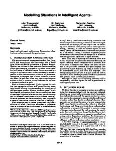
Let us now come back to the processing rate (2.2) given by r(x) = µx/(a + x). This expression has been derived in the previous section using physical considerations. It is well known however, that the queueing theory studies precisely the single server problem. Is it therefore possible to find a link between this theory and the processing rate (2.2)? Before answering this question, let us first recall the basic queueing theory principles and notations (see for instance [116] for an introduction). A generic queueing environment is described in the form A/B/c, where the first two descriptors A and B connote the arrival and service statistics, respectively, and the third descriptor c connotes the number of servers. If the total number of customers† in the queueing systems is denoted N , the mean, steady state customer arrival rate λ and the mean time spent by each customer in the system T , then, an important result, known as the Little’s theorem may be stated as follows : N = λT This is indeed quite intuitive and it holds generally for a wide range of service disciplines and arrival statistics. One of the best understood class of queueing systems is the M/M/1 case where M stands for memoryless. An arrival rate, with rate λ, is said to be memoryless if the probability of the number of arrivals in some subinterval [t, t + τ ] is given by a Poisson distribution as follows : eλτ (λτ )k k! The probability distribution of the time interval between two successive arrivals is then given by an exponential distribution with expected value 1/λ. This exponential distribution is memoryless, i.e. we have that the additional time needed to wait for an arrival is independent of past † We are of course concerned with network packets but the use of the word customer is widespread in queueing theory.

34

Chapter 2. Fluid flow modelling of a FIFO buffer

history. Let the random process N (t) denotes the time evolution of the total number of customers in the system and define :
x ¯ = lim E N (t) t→+∞

It can be shown using queueing theory results that x ¯=

λ µ−λ

(2.6)

where µ is the average service rate of the buffer server. Using the Little’s formula, it follows that the average time spent by each customer in steady state is given by : 1 T = µ−λ Using the mass balance equation (2.3) and the processing rate (2.2), we find that, for a constant input rate λ = v(t) < µ, the system (2.3)-(2.2) has a single equilibrium given by (see Fig. 2.2) : λ=

µx a+x

or

x=

aλ µ−λ

For a = 1, we then recover the classical formula (2.6) of queueing theory for M/M/1 systems. The fluid-flow model x˙ = v(t) −

µx 1+x

may therefore be interpreted as an approximate dynamical extension of the steady-state result given by the queueing theory. Although not widely spread, this model has been used in [92] for deriving a nonlinear adaptive network controller. A comparison between the integrated model and actual data is also provided. Further references may be found in [114]. It has been shown in [87] that a Poisson model is however a bad choice for network analysis. As we will see later, this is not a limitation of our model as the parameter a may be used to fit a given λ, x ¯ steady-state relationship.

2.2.1

Illustration

Consider the following experiment : A network buffer with average service rate µ = 40 packets per second [pps] is fed by a source with exponentially distributed inter-packet arrival time whose average rate jumps every Ts = 10 seconds from a value of 10 [pps] to a value of 15 [pps]. This experiment is carried out on a discrete event queue simulator and

2.2. Queueing theory perspective

35

repeated five thousand times so as to obtain the ensemble average of the buffer load at regular time intervals. The result is shown in Fig. 2.7(A) (light curve). It is clear that the average buffer load is non-zero and increases when the average input rate increases. If the fluid flow input rate v(t) is chosen as :  10 kTs 6 t < (k + 1)Ts v(t) = (2.7) 15 (k + 1)Ts 6 t < (k + 2)Ts k = 0, 2, . . . integrating the system (2.3)-(2.2) with a = 1 and the input rate given by eq. (2.7) yields the curve shown in Fig. 2.7(A) (dark curve) which is compared with the curve obtained with the discrete event queue simulator (light curve). It is clear that our fluid model reproduces the desired behaviour. Not only does our model converge in steady state toward the value predicted by the queueing theory but it may also be observed that the transient periods are well reproduced.

2.2.2

Relationship with other processing rate functions

A number of models may be found in the literature for the FIFO queue shown in Fig. 2.1. As we have seen already, model (1.2) is a discrete version of the mass balance equation (2.3). Another widely used continuoustime fluid-flow model may be found for instance in [13] and [10]. Although they do not use the concept of processing rate, this model may be expressed using this notion as follows :  µ if x > 0 r(x(t), v(t)) = (2.8) min(µ, v(t)) if x = 0 The processing rate (2.8) with the mass balance equation (2.3) expresses that, as long as the input rate is smaller than the link capacity µ, the buffer level is equal to zero and the output rate is instantaneously equal to the input rate. The buffer level increases or decreases at a rate v(t)−µ if the buffer is not empty. Let us consider again the illustrative experiment mentioned above. In this setup, the link capacity was set to µ = 40 and the input rate was set to v(t) = 10 or v(t) = 15. Hence, the integration of model (2.3)-(2.8) would give a buffer level always equal to zero which is in contrast with our proposed processing rate which reproduced the behaviour predicted by the queueing theory shown in Fig. 2.7(A). In order to compare the processing rate (2.2) and (2.8), let us consider another experiment. The model (2.3)-(2.2) is integrated with µ = 15 and  20 t < 1 v(t) = 5 t>1

36

Chapter 2. Fluid flow modelling of a FIFO buffer

x [p] 0.7 0.6 0.5 0.4 0.3 0.2

Fluid Flow Model

0.1

Discrete event simulator

0 0

10

20

30

40

50

60

70 time [s]

(A) buffer load [p] x 9

24

[pps]

8

20

7

16

6

12 8

5

4

4 3

0 0

1

2

3

4

a=0.01

1

decreasing value of a 0

1

5 [s]

a=1

2

0 −1

input rate u(t)

2

3

4

5 time [s]

(B) Figure 2.7: (A) Comparison between a discrete event queue simulator and the simulation with the fluid-flow model (2.3)-(2.2) (B) Average buffer queue length for different value of the parameter a when the input rate is greater than the link capacity during one second.

2.3. (Min,+) theory perspective

37

for different values of the parameter a. The model (2.3)-(2.8) is then integrated under the same conditions. The comparison is shown in Fig. 2.7(B) where the curve corresponding to the processing rate (2.8) is displayed in dotted line. For a tending toward zero, the processing rate (2.2) approximates a step function and therefore both models give very similar results. This situation corresponds to a linear increase followed by a linear decrease of the buffer level. This therefore corresponds to a situation where the stochastic effects are not taken into account and where the queueing delay is null at equilibrium. Our fluid flow model can therefore be made arbitrarily close to a model with a discontinuous processing rate function which is often used in the literature and which corresponds to a deterministic case. The precise relationship that exists between the value of the parameter a and the probability distribution of the input rate will not be analysed further in this text. Indeed, the model constructed in this thesis is to be used to obtain insight into the dynamical behaviour of a given strategy and not for quantitative purposes. Furthermore, the control law presented in this text will be shown to be model independent and the stability analyses will be carried out for all values of a > 0.

2.3

(Min,+) theory perspective

(Min,+) algebra, known as network calculus in this context, has been highly successful in describing systems where flows are reshaped by some service disciplines (see [63, 1] and the annex A ). In particular, the FIFO buffer displayed in Fig. 2.1 is known in this theory as the constant bit rate (CBR) server. Once again, we would like to know if the description provided by the network calculus can be related to the fluid-flow models described so far and more precisely how it relates to the processing rate (2.2). In (Min,+) algebra, the traditional algebraic structure (R, +, ×) is replaced by (R ∪ {+∞}, ∧, +) where ∧ stands for the minimum (or the infimum if it does not exists) and + remains the traditional addition operator. It can be easily verified that this structure is a commutative dioid. Network calculus uses the notion of accumulated rate. The accumulated departure rate corresponding to Fig. 2.1 is given by : Z W (t) =

t

w(t) dt 0

In this section, capital letters will be used to denote accumulated rates. Consider a constant bit rate server with a service rate of µ packets per second. The number of packets emitted by such a server queue over any

38

Chapter 2. Fluid flow modelling of a FIFO buffer

time interval τ is limited by : W (t) − W (t − τ ) 6 µτ

06τ 6t

(2.9)

Inequality (2.9) may then be rewritten W (t) 6 µτ + W (t − τ ) 0 6 τ 6 t

which implies that : W (t) 6

inf (µξ + W (t − ξ))

66

0 ξ t

Rt If the accumulated arrival rate at the buffer is denoted V (t) = 0 v(t) dt, with v(t) the input rate, and if the buffer is supposed to release packets as fast as the service discipline allows it, it may be shown that the accumulated departure rate is given by W (t) = inf (µξ + V (t − ξ))

66

0 ξ t

Recalling that (Min,+) algebra translates the conventional addition into the minimum operator and the multiplication into addition, we can easily recognise in this formula the usual convolution operator. This formula indeed corresponds to the (Min,+) convolution denoted ⊗ and may therefore be rewritten : W (t) = R(t) ⊗ V (t)

(2.10)

with R(t) = µt for a constant bit rate server. That is to say that (2.10) is the network calculus model corresponding to the FIFO buffer shown in Fig. 2.1. The question of interest in this Section is to find out if there is a system of the form : x˙ = v(t) − r(x, v) with input v(t) and output w(t) = r(x(t, v(t))), W (t) = which satisfies equation (2.10) ?

2.3.1

An equivalent (Min,+) system

Consider the function : L(t, ξ) = µ(t − ξ) + V (ξ)

Rt 0

w(t) dt and

2.3. (Min,+) theory perspective

39

3.2

2.8

L(t, ξ)

2.4

2.0

µ(t − ξ)

1.6

µ

1.2

V (ξ)

0.8

t=2

0.4

0 0

0.2

0.4

0.6

0.8

1.0

1.2

1.4

1.6

1.8

ξ∗

2.0

ξ

Figure 2.8: Graphical representation of the (min,+) convolution depicted for t = 2

and let’s define W (t) =

inf L(t, ξ)

66

0 ξ t

= L(t, ξ ∗ ) = µ(t − ξ ∗ ) + V (ξ ∗ ) with ξ ∗ (t) = arg.min06ξ6t µ(t − ξ) + V (ξ). With these notations, it is clear that W (t) is indeed the result of a (Min,+) convolution as given by eq. (2.10). Consider the equations : x(t) = V (t) − W (t) = V (t) − µ(t − ξ ∗ (t)) − V (ξ ∗ (t)) taking the time derivative on both side of the equality ∂ξ ∗ (t) ∂ξ ∗ (t) ∂x = v(t) − µ + µ − v(ξ ∗ (t)) ∂t ∂t ∂t

(2.11)

As illustrated in Fig. 2.8 which graphically represents the convolution operation, possible value for ξ ∗ are at the boundaries of the interval

40

Chapter 2. Fluid flow modelling of a FIFO buffer

[0, t] or strictly inside at the points where : ∂L(t, ξ) ∂V (ξ) = 0 or µ = v(ξ) = ∂ξ ∂ξ ∂L(t, ξ) does not exist. ∂ξ Obviously, these points are, except for ξ ∗ = t (the right boundary of the interval), independent of t which yields :

or are located at the points where

∂ξ ∗ ∂t ∂ξ ∗ ∂t

= 0 if ξ ∗ 6= t = 1 if ξ ∗ = t

Therefore, system (2.11) may take the following two forms : x˙ = 0 ξ ∗ = t x˙ = v(t) − µ

ξ∗

6= t

(2.12) (2.13)

It remains to specify when the switches occur between the two systems. Switching between (2.13) and (2.12) A necessary condition for a switch to occur at time t between (2.13) and (2.12) is obviously that L(t, ξ ∗ ) = L(t, t)

(2.14)

that is to say that the minimum with respect to ξ of the curve L(t, ξ) is equal to the value reached by that curve for ξ = t. As we know that L(t, ξ ∗ ) = W (t) and that L(t, t) = V (t), condition (2.14) may be rewritten as V (t) = W (t) or x = 0 Provided that condition (2.14) is satisfied, a switch will occur between (2.13) and (2.12) depending on the time evolution of the quantities V (t) and L(t, ξ ∗ ). By definition ∂V (t) = v(t) ∂t and for a point ξ ∗ ∈ [0, t[, we have that ∂L(t, ξ ∗ ) =µ ∂t

2.3. (Min,+) theory perspective

41 v(t) < µ x=0

x˙ = 0

x˙ = v(t) − µ

w(t) = v(t)

w(t) = µ

v(t) > µ Figure 2.9: Hybrid system view of the convolution (2.10)

Therefore, the hybrid system depicted in Fig. 2.9 is equivalent to the (Min,+) convolution (2.10). The system switches from eq. (2.12) to eq. (2.13) when v(t) > µ, x = 0 and from (2.13) to eq. (2.12) when v(t) < µ, x = 0. Furthermore, it is easy to verify that the hybrid system depicted in Fig. 2.9 is also equivalent to a fluid flow model x˙ = v(t) − r(x, v) with r(x, v) given by eq. (2.8).

2.3.2

Relationship with the processing rate (2.2)

A natural question is now to ask whether or not it is possible to find a function R(t) so that the convolution (2.10) is equivalent to the system (2.3) with processing rate function (2.2) In fact, it is easy to show that such a function R(t) does not exist. Consider two input functions v1 (t) and v2 (t) with their respective accumulated arrival rate V1 (t) and V2 (t), we have that W1 (t) = V1 (t) ⊗ R(t) W2 (t) = V2 (t) ⊗ R(t) Consider V3 (t) = V1 ∧ V2 where ∧ is the minimum operator. Define the function W3 as follows :
W3 (t) = V1 ∧ V2 ⊗ R(t)

= V1 ⊗ R(t) ∧ V2 ⊗ R(t) = W1 (t) ∧ W2 (t)

42

Chapter 2. Fluid flow modelling of a FIFO buffer

[p]

[p]

100 90 80 70 60 50 40 30 20 10 0

80 ff

W1

70 60 50 40 30

Wff 2

Wff 3

20 10 0 0 0.1 0.2 0.3 0.4 0.5 0.6 0.7 0.8 0.9 1.0

w1

w2 = w3

0 0.1 0.2 0.3 0.4 0.5 0.6 0.7 0.8 0.9 1.0 [t]

[t]

(a) Processing rate function (2.2)

(b) Processing rate function (2.8)

Figure 2.10: Numerical counter example for the distributivity of the minimum w.r.t the convolution operation for system (2.3)-(2.2) and illustration of the same property for system (2.3)-(2.8)

which holds by distributivity of the convolution operator w.r.t the minimum. Now, consider the three systems below and the corresponding accumulated departure rate : W1f f =

Rt

x˙ 1

= v1 (t) − r(x1 )

x˙ 2

= v2 (t) − r(x2 ) W2f f = 0 r(x2 (τ ))dτ
Rt d = V1 ∧ V2 − r(x3 ) W3f f = 0 r(x3 (τ ))dτ dt

x˙ 3

0

Rt

r(x1 (τ ))dτ

A necessary condition for system (2.3) with processing rate function (2.2) to be written under the form of a (Min,+) convolution is therefore that : W3f f = W1f f ∧ W2f f Fig. 2.10(a) shows a numerical counter-example of that property. The functions used are V1 (t) = 150t, V2 (t) = 20 + 50t and µ = 100.The parameter a is set to 10 so that the effect is clearly visible in the figure. It can also be verified in Fig. 2.10(b) that the property above is indeed verified if the processing rate function (2.8) is used. Although it is not possible to find an exact function R(t) that fulfils the goal stated above, it is still of interest to have an idea of a function R(t) which would approach such a goal. To that end, consider a single trajectory of system (2.3)-(2.2) obtained with a constant input rate λ < µ and initialised with x(t = 0) = 0. For small value of x, the processing

2.4. Conclusion

43

rate function (2.2) may be written as : r(x) ≈ µx and therefore λ (1 − e−µt ) µ r(x(t)) ≈ λ(1 − e−µt ) x(t) ≈

Define, as usual, Z Wrx (t) =

t

r(x(t))dt 0

= λt +

λ −µt (e − 1) µ

Fig. 2.11 compares this function W (t) with two functions obtained as follows : Wcbr = λt ⊗ Rcbr (t) Rcbr = µt Wdelay = λt ⊗ Rdelay Rdelay = max {0, λ(t − µ1 )} That is to say the output of a constant bit rate server with service rate µ and the output of a constant bit rate server with pure delay 1/µ and service rate λ. The vertical deviation between Wcbr and Wrx is equal to quantity x(t) of information in the buffer. The horizontal deviation corresponds to the associated queueing delay. As described in Section 2.2, this queueing delay account for the asynchronous nature of packets arrival in queueing networks. It should be noted here that it would be more natural to compare the function Wrx with a constant bit rate server with delay 1/µ. Instead, we have compared it with a constant bit rate server with service rate λ and delay 1/µ. For the latter system, a transient queueing delay exists which corresponds to the accumulation of packet in the queue during the delay. If the service rate µ is greater than the arrival rate λ, the output rate remains equal to µ until the queue is empty. For such a system, the steady delay is null. By contrast, our model takes into account a steady state queueing delay due to the stochastic nature of the input stream.

2.4

Conclusion

A non-linear fluid flow model suitable for representing a large class of queueing systems has been presented. This model was shown to be

44

Chapter 2. Fluid flow modelling of a FIFO buffer

5 4 3 λt

2

max(0, λ (t−µ1 ))

1 Wrx (t)

0 0

1 µ

0.1

0.2

0.3

0.4

0.5 [t]

Figure 2.11: Comparison between the approximative accumulated departure rate (dashed curve) of system (2.3)-(2.2) and the accumulated departure rate obtained with a constant bit rate server (top curve) and a constant bit rate server with pure delay 1/µ (bottom curve) as seen by the (Min,+) theory

an approximate non-stationary extension of the results given by the queueing theory. Depending on the choice of a model parameter, it was also shown that our fluid flow model could as well be seen as a smooth approximation of a model widely used in the network control literature which is itself identical to the CBR server used in network calculus.

Chapter 3

Application: Optimal fluid flow control of a FIFO buffer A general fluid flow model for a network buffer was presented in the previous chapter and shown to be suitable for representing a large class of queueing systems . This model is now extended to take into account the tail drop queueing policy discipline. An on-line identification scheme for this model is presented and an optimal control strategy is developed using the minimal principle of Pontryagin. Experimental results show that the implementation of this control policy is nearly optimal for a wide range of experimental conditions. Some parts of this chapter may be found in [35].

3.1

Fluid flow model with tail-drop policy

Consider the system depicted in Fig. 3.1 showing a typical management scheme of a network buffer. In this setup, a quantity w(t) of packets per second arrives in the system. Depending on the number x(t) of packets already waiting in the buffer and on the service rate µ of the network server, it may be desirable to drop a fraction of this incoming flow to prevent network congestion. The incoming flow w(t) is therefore split into two flows: a flow d(t) of dropped packets and a flow u(t) actually fed to the network buffer. 45

46

Chapter 3. Application: Optimal fluid flow control of a FIFO buffer

x

arriving packets

w

u

departing packets

v Buffer

d dropped packets

Figure 3.1: A simple network buffer. Packets arrive at a rate w(t), a quantity d(t) of packets per second is lost and the remaining flow u(t) is fed to the buffer.

The separation of the input stream w(t) (Fig. 3.1) between a stream of dropped packets d(t) and a stream u(t) actually fed to the buffer is mainly motivated by two conflicting criteria : On one hand, the number of dropped packets in a network should be kept as small as possible to avoid retransmission but on the other hand, the transmission of large bursts requires large queues which increases the transmission delay. This trade-off is captured in the following function : L(x, t, u) = x(t) + Rd(t) = x(t) + R(w(t) − u(t)) with R > 0, a positive weight on the dropping rate and x(t) the buffer length which is indeed proportional to the queueing delay. Therefore, we consider the cost function : Z tf J(x, tf , u) = L(x, t, u)dt (3.1) 0

The minimisation of this cost function is considered in Section 3.2.

3.1.1

Tail-drop policy

The most basic queueing strategy used as the default queueing discipline on most systems is known as tail-drop. When packets arrive into a queue faster then the queue is able to process them, packets are queued in order to wait for service. This accumulation allows the packets to successfully arrive at their destination without being dropped because of temporary lack a resources. As mentioned above, this positive effect is obtained at the expense of a longer queueing delay in the system. The number of packets allowed to be queued must however be limited. First, packets waiting in a router occupy memory which is a limited resource. Second, maintaining unreasonably long queues results in unacceptable delays.

3.2. Optimal control

47

Therefore, a fix threshold is usually associated with a queue. Packets are allowed to be accumulated until the queue occupancy reaches this threshold at which point further arriving packets are discarded. In this chapter, the control parameter is the input stream u(t) actually fed to the buffer. It will be shown that the optimum strategy can be expressed as an optimal profile for the buffer occupancy. The threshold mentioned above will therefore be used in order to control the measured value of the buffer occupancy toward the optimum value which will result in an adaptive threshold control.

3.2

Optimal control

The optimal control problem can be stated as follows : Given the system

x˙ = f (x, t) = u(t) −

µx a+x

0 6 u(t) 6 w

(3.2)

with d(t) = w − u(t), find the optimal control u∗ (t) which minimises the cost function (3.1) along the trajectories of system (3.2). The control problem is envisioned for an input rate smaller than the buffer capacity µ but which sometimes has bursts of short duration and of constant amplitude w greater than µ. The solution of this minimisation problem is a direct application of the minimum principle of Pontryagin (see for instance [12]). The Hamiltonian with costate p (which plays the role of Lagrange multipliers in convex optimisation) is as follows :

H(x, t, u) = L(x, t, u) + pf (x, t)   = x(t) + R w − u(t)  µx  +p u(t) − a+x

The minimum principle of Pontryagin then states that the optimal con-

48

Chapter 3. Application: Optimal fluid flow control of a FIFO buffer

trol must satisfy the following conditions : x˙ p˙ minu H(x∗ , u, p∗ ) ∂ˆ g { − p}tf ∂x {H +

∂ˆ g }t ∂t f

∂H ∂p ∂H = − ∂x

=

(A) (B)

= H(x∗ , u∗ , p∗ ) (C) = 0

(D) or

= 0

(E)

These conditions can be derived using the Fundamental Theorem of the Calculus of Variations. Given the definition of the Hamiltonian, condition (A) simply states that the optimal trajectories must satisfy the dynamics (3.2). Condition (B) gives the evolution of the costate p and condition (C) indicates that the optimal control must minimise the Hamiltonian along the optimal trajectories. Condition (D) is usually used to find the initial condition for (B) and (E) may be used to compute the final time tf . The function gˆ can be used to take into account a terminal cost or to take into account some constraints on the state. This function is identically equal to zero in our particular setup. Conditions (A), (B) and (C) may be rewritten in this particular case : x˙ = f (x, t)

aµ (a + x)2 = arg.min0≤u(t)≤w H(x∗ , t, u)

p˙ = −1 + p u∗

3.2.1

Minimisation of the Hamiltonian

The partial derivative of the Hamiltonian with respect to u is given by : ∂H(x, t, u) =p−R ∂u Minimising the Hamiltonian with respect to u therefore yields  p>R  0 ∗ w p
3.2. Optimal control

49

This optimal control is known as “Bang-Bang” as the optimal control “bangs” on its maximal and minimal values. Note that this is obviously a general result for system with an Hamiltonian linear in u. It has been shown already in [94] that the optimal control of a fluid flow buffer is of the bang-bang type using a different fluid flow model and different constraints on the control. Defining s(t) = p(t) − R, a singular arc on a time interval [t1 , t2 ] will be obtained if di s (x, p)p=R = 0 ∀i ∈ N ∀t ∈ [t1 , t2 ] dti Let us compute the time derivatives •

ds dt

=

dp dt

d2 s dt2

and

d2 s dt2

aµ = −1 + p (a+x) 2

ds ∗ ∗ (x , p )p=R = 0 dt •

ds dt

⇐⇒

x∗ =

p

aRµ − a

aµ −2aµ = p˙ (a+x) ˙ 2 + p (a+x)3 x

d2 s ∗ ∗ (x , p )p=R = 0 dt2

⇐⇒

x˙ x=x∗ = 0

⇐⇒

using = using

µx∗ a + x∗ r a ) = µ(1 − Rµ

i

i

It is readily seen that, if ddtsi (x, p)p=R = 0 for i = 1, 2 then ddtsi (x, p)p=R = 0 for all i. Therefore, the singular arc (of order 2) is characterised by p˙ = x˙ = 0 xsing =

p aRµ − a

using =

µxsing a + xsing

(3.3)

The optimal control is therefore a succession of time intervals where the control variable u takes its maximal value u = w (MAX), its minimal value u = 0 (MIN) or its singular value using (SING). On the singular arc, both the costate and the state take a constant value given by (3.3). Whenever the singular arc is reached, the costate takes a constant value equal to R and the system remains on this arc. However, the singular arc must finally be left in order to satisfy some final conditions.

50

Chapter 3. Application: Optimal fluid flow control of a FIFO buffer

3.2.2

Boundary conditions

The formulation of the optimisation must be completed with the boundary conditions (D) and (E). These conditions are stated here with the idea that we are looking for the optimal control path when the input rate w(t) represents a burst, that is to say a function of the type :  w t ≤ tburst w(t) = (3.4) 0 otherwise The control period [t0 , tf ] is therefore envisioned to be larger than the burst duration. The initial condition x0 = x(t0 ) is given. Additional conditions depend on the formulation of the problem : 1. Final time tf fixed, x(tf ) free: In this situation, the additional condition is on the final value of the costate : p(tf ) = 0 The following alternative formulation may also be considered. 2. Fixed final state value x(tf ) with x(tf ) small, tf free. The final time tf is given by : H(x(tf ), tf , u(tf )) = 0 The integration of the dynamics of the system yields the final time tf and the above relationship may then be used to determine the final value of the costate. We next consider an example where the optimal control is of the MAX-SING-MAX type.

3.2.3

Example

Let us now consider an illustrative example of an M/M/1 queue fed at a rate w(t) given by eq. (3.4) with w = 60 and tburst = 1. The average service rate is set to µ = 50. The optimisation problem is considered with a fixed time interval [0, tf = 1.3]. The weight R is set to 0.2. The results are shown in Fig. 3.2 where the average buffer length x, the optimal control u∗ and the costate p are displayed. The optimal control presents three distinct stages : In the time interval [t0 , t1 ], the control u is set to its maximal value to allow the state variable x to reach its singular value x∗ as quickly as possible. Once the singular arc is reached, the system is controlled so

3.2. Optimal control

51

that p˙ = 0 and x˙ = 0 and the system therefore stays on this arc during the time interval [t1 , t2 ]. The singular arc must eventually be left in order to satisfy the boundary condition p(tf ) = 0. The time instant t2 may be determined iteratively by ”shooting” from selected initial instants. With this profile, the optimal cost calculated with eq. (3.1) is 6.49. This number may be compared in Fig. 3.3 with different costs obtained with a tail-drop policy for different value of the threshold. With this policy the minimum cost is given for a threshold set at 2.42 and is 7.01. Clearly, a substantial improvement is obtained using the optimal profile. However, it must be noted that the computation of the time instant t2 requires the a priori knowledge of the burst duration which is not known in practice. This problem is further discussed in Section 3.3.

3.2.4

Other optimum scenari

Besides the typical MAX-SING-MAX control presented in Fig. 3.2, one may also encounter the following scenari : 1. if w < using , No singular control is possible, depending on the evolution of the costate, the Optimal control can be of two types: • MIN-MAX : This situation is illustrated in Fig. 3.4 showing the costate coming from a value greater than R toward zero. This scenario is obtained with the following parameters (using =40): µ = 50 R = 0.5 w = 30

x0 = 150 tf = 1

• MAX : This situation is illustrated in Fig. 3.5 showing the costate which is never greater than R. This scenario is obtained with the following parameters (using = 45): µ = 50

R = 2 w = 30 x0 = 0 tf = 1

2. if w ≥ using , singular control is possible, depending on the initial condition x0 , the optimal strategy can be MAX-SING-MAX or • MIN-SING-MAX : If we now start off with a value x0 greater √ than x∗ = Rµ − 1, the optimal strategy is to decrease x in order to reach the singular control as fast as possible. This decreasing period will of course be obtained for u = 0 as illustrated in Fig. 3.6 showing the optimal control when x0 = 20

52

Chapter 3. Application: Optimal fluid flow control of a FIFO buffer

6 Average buffer load

5 4 3 2 1 0 0

0.2

0.4

0.6

0.8

1.0

1.2

1.4

60 Actual Input rate u(t) 50 40 30 20 10 0 0

0.2

0.20 0.18 0.16 0.14 0.12 0.10 0.08 0.06 0.04 0.02

0.4

0.6

0.8

1.0

1.2

1.4

0.6

0.8

t21.0

1.2

1.4

costate p

0 0

t10.2

0.4

time[s]

Figure 3.2: Optimal control in the presence of a burst.

3.2. Optimal control

53

7.5 7.4

Cost versus threshold

7.3 7.2 7.1

singular value 2.16

2.42 ×

7.0 2.0 2.2 2.4 2.6 2.8 3.0 3.2 3.4 3.6 3.8 4.0

7.03 7.01

Figure 3.3: Cost for different values of the threshold under tail-drop policy. The optimal profile gives an optimal cost of 6.49.

151 147 143 139 135 131 127 123 119 115 1.0 0.9 0.8 0.7 0.6 0.5 0.4 0.3 0.2 0.1 0

buffer occupancy

0 0.1 0.2 0.3 0.4 0.5 0.6 0.7 0.8 0.9 1.0 costate p

R

0 0.1 0.2 0.3 0.4 0.5 0.6 0.7 0.8 0.9 1.0 time [s]

Figure 3.4: Illustration of the MIN-MAX optimal control.

54

Chapter 3. Application: Optimal fluid flow control of a FIFO buffer

1.6 1.4 1.2 1.0 0.8 0.6 0.4 0.2 0 0.13 0.11 0.09 0.07 0.05 0.03 0.01 −0.01

buffer occupancy

0 0.1 0.2 0.3 0.4 0.5 0.6 0.7 0.8 0.9 1.0 costate p

0 0.1 0.2 0.3 0.4 0.5 0.6 0.7 0.8 0.9 1.0 time [s]

Figure 3.5: Illustration of the MAX optimal control.

60 50 40 30 20 10 0 120 100 80 60 40 20 0

buffer size

0

1

0

1 t1

2 3 optimal control u*

2

3

4

4 t2

5

5 time [s]

Figure 3.6: Illustration of the MIN-SING-MAX optimal control.

3.2. Optimal control

55

• No singular control : The time instants t1 and t2 shown in Fig. 3.2 and 3.6 are calculated as follows: t1 is the time needed for the state variable x to go from its initial value x0 to the value x∗ . The time instant t2 is tf − t3 where t3 is the time needed for the costate p to go from a value of R (and x starts at x∗ ) to a value of zero. Therefore. it may well be the case that t1 + t2 > tf . In this case, there is no singular control and the optimal strategy if one of MIN-MAX or MAX.

3.2.5

Integration method

The evolution of the costate is calculated with a simple “shooting technique”. Recall that condition (D) gives the value of the costate at time t = tf . In order to find the initial costate p(0) = p0 , one has to integrate the system with different initial values until one trajectory ends at the desired final value for the costate, hence the term “shooting”. Given condition (D), this problem is equivalent to finding the zero of the function fp : p0 fp = p(tf ). The following algorithm uses the Newton-Raphson method and has been successfully used in all examples given in this chapter : tol=1e-4; er=2*tol; // something greater than tol p0=0.1; // guess intial p0 p0_k =p0; while (|er| > tol) { // start at (x0,p0_k) [x1;p1] = integrate_the_system([x0;p0_k]); // start at (x0,p0_k+h) [x2,p2] = integrate_the_sytem([x0;p0_k+h]); pT_k = p1(tf); pT_kh = p2(tf); p0_knext = p0_k - pT_k*(h)/(pT_kh-pT_k); p0_k = p0_knext; er = pT_k; }

// Newton

56

Chapter 3. Application: Optimal fluid flow control of a FIFO buffer

This algorithm computes the root of the function ( fp : p0

fp = p(tf ) with

∂H p(0) = p0 ∂x x˙ = f (x, t) x(0) = x0 p˙ = −

using the Newton-Raphson method. The derivative of fp with respect to p is approximated by (fp (p + h) − fp (p))/h.

3.3

Implementation of the optimal control

The computation of the optimal control requires the integration of the costate equation and the system dynamics. As pointed earlier, the burst duration itself must be known to calculate the optimal profile. In order to obtain a useful control law, the optimal strategy should be described as a feedback of some state measurement which would make it robust to model uncertainties and should not rely on a-priori knowledge on the traffic characteristics. A closed loop control is easily obtained if the final interval [t2 , tf ] is neglected. In this case, the optimal strategy becomes identical to the tail-drop policy which only requires the measurement of the state x. The control law therefore reduces to the tracking of the singular value xsing given by eq. (3.3). For the example given above, xsing = 2.16. The effect on the cost may be observed in Fig. 3.3. It can be seen that this value yields a suboptimal cost which lies in the vicinity of the best cost obtained under tail-drop policy. An idea of the importance of the neglected interval is obtained if we consider a burst with tburst greater than tf . In that case the processing rate function (2.2) is approximated by r(x) = µ and the costate evolution by p˙ = −1. An explicit value for t2 is t2 = tf − R which indicates that the singular arc should be left earlier if the weight on the dropping rate is increased. If the last interval is to be neglected, the parameter R should therefore be small compared to a typical burst duration. Note that, if short bursts occur and if an important weight is set on the dropping rate, a sensible policy would be to accumulate the entire burst in the buffer and prevent any overflow to occur. Our sub-optimal control can now be stated : 1. Obtain fluid-flow measures of needed variables: • x ˆ: Estimate of the average buffer length ˆ Estimate of the rate of packets through the buffer • λ:

3.3. Implementation of the optimal control

57

2. Obtain an estimate a ˆ of the parameter a 3. Compute q the singular values: xsing = a ˆ ) µ(1 − Rµ

√ Rµˆ a−a ˆ and using =

ˆ > using , drop packets so as to control x 4. if λ ˆ at its singular value xsing These steps are now described in the following Subsections.

3.3.1

Fluid flow measures

Fluid-flow variables are measured with a sliding window of length ∆ [sec]. During these ∆ seconds, the number of outgoing packets N and the sum τ of the seconds spent by each packet in the system is recorded. Variables are estimated as follow : ˆ = λ Tˆ =

N ∆ τ N

: average rate : average retention time

The average buffer length is then calculated using the Little’s formula[56] : ˆ Tˆ = τ x ˆ=λ ∆

3.3.2

On-line model identification

The computation of the singular value xsing requires the knowledge of the parameter a which depends on the stochastic properties of the traffic. It is therefore necessary to estimate this parameter on the basis of some traffic measurements. ˆ k ), k = 1, . . . , K, Given a set of K measurement vectors pk = (ˆ xk , λ it is easy to show that the value aest that best fits the processing rate (2.2) in the sense aest = arg.mina

K X i=1


µˆ xi ˆi 2 −λ a+x ˆi

is given by : aest

= =

µ

PK

ˆi i=1 x

−

PK

PK ˆ i=1 i=1 λi

K µΨK x − Ψxλ ΨK λ

ˆi x ˆi λ

58

Chapter 3. Application: Optimal fluid flow control of a FIFO buffer

K K where the variable ΨK x , Ψxλ , Ψλ are introduced for convenience. Therefore, the following method for the estimation of the parameter a is proposed : Every ∆ seconds compute

ΨK x

= ΨK ˆ x +x

K ˆ ΨK ˆλ xλ = Ψxλ + x ˆ ΨK = ΨK + λ λ

λ

aest = (µΨK x − Ψxλ )/Ψλ a ˆ = a ˆ + h(aest − a ˆ)

The successive estimate aest are filtered with a gain h < 1 to avoid rapid change between estimations of a. The parameter a is evaluated ˆ This is not every ∆ which is the value used for the estimation of x ˆ and λ. required but minimises the number of parameters used for the algorithm. This method is illustrated in Fig. 3.7 showing the convergence of the estimated value of a toward its theoretical value. This figure is obtained with the OMNET++ [115] simulator with the following parameters : ∆ = 5[s], µ = 500[pps], h = 0.5 In order to obtain a suitable excitation of the system during the identification, the input rate is changed every 10 seconds. The following two values are used recursively: 1/0.003, 1/0.005 In the M/M/1 case, the estimation a ˆ converges toward 0.98 which is close to the theoretical value 1. In the M/D/1 case, the relationship that links the number of customers in the system as a function of the rate λ is given by p λ = (1 + x) − 1 + x2 (3.5) µ It is easy to verify numerically that the value of a that minimises the distance between (2.2) and (3.5) is close to 0.63. The convergence of a ˆ toward 0.7 indicates that the system has been successfully self-adapted to the M/D/1 situation.

3.4. Simulation results

59

2.0 1.8 Estimation of the parameter a

1.6 1.4 1.2

M/M/1 0.98

1.0 M/D/1

0.8

0.7

0.6 0

40

80 120 160 200 240 280 320 360 400 time [s]

Figure 3.7: On-line estimation of the parameter a of the proc. rate (2.2) in the M/M/1 and M/D/1 case. Initial estimation is set to a ˆ(0) = 2

3.3.3

Adaptive threshold

In order to regulate the average queue length at its singular value, an adaptive threshold c is used. This threshold is used at every packet arrival to decide if the packet should be enqueue or dropped. The parameter c is updated, once again, every ∆ seconds, so as to keep the average buffer length within ten percent of the tracked value : the operation is as follows : ˆ > using ) if (λ if x ˆ > 1.1xsing : if x ˆ < 0.9xsing :

c=c−1 c=c+1

With this algorithm, the control strategy is triggered only when the rate through the buffer is larger than the singular value. The adaptive threshold will maintain the average buffer load around the singular value xsing .

3.4

Simulation results

Experimental results are obtained with the OMNET++ simulator. The source uses exponentially distributed inter-packet delay (Poisson source) whose average changes periodically, every T = 10 seconds. The values 0.005,0.0009, 0.005 and 0.0005 are used recursively to obtain some rates of 200, 1111, 200 and 2000 [pps].

60

Chapter 3. Application: Optimal fluid flow control of a FIFO buffer

Cost

20 Experimental result

19 18 17 Cost obtained with adaptive threshold

16 15 1

3

5

7

9

11

13

15

Threshold

Figure 3.8: Cost obtain with the adaptive threshold control compared to the costs obtained with a constant threshold for different values of this threshold (costs are averaged over 10 experiments).

The service time is also exponentially distributed, its average is set to 0.001 (µ = 1000 [pps]). The fluid-flow variables are updated every ∆ = 1 [s]. The weight on the dropping rate is set to R = 0.1 and the filter gain is h = 0.5. The average buffer load x ˆ, the singular value xsing and the adaptive threshold c obtained with the control strategy presented in this chapter ˆ is also displayed are displayed in Fig. 3.4. The estimated throughput λ with the calculated singular value using showing the time interval where the control law is active. It can be verified that the threshold is successfully adapted so as to bring the average buffer load in the vicinity of the tracked value. Fig. 3.8 offers a comparison between the cost obtained with the adaptive threshold and the different costs obtained with a constant threshold. As expected, our adaptive control law operates the system so as to yield a cost approaching the best cost obtained with a constant threshold. The costs are averaged over 10 experiments.

3.4. Simulation results

61

12

xsing

ixhat x_star threshold

threshold

10

8

6

4

^x

2

0 0

10

20

30 time [s]

40

50

60

1200 lambdaihat u_sing

using

1000

800

600

^λ

400

200

0 0

10

20

30 time [s]

40

50

60

Figure 3.9: top:Average buffer length x ˆ, tracked value xsing and adaptive threshold ˆ c. Bottom: Estimated throughput λ and singular value using . The adaptive threshold is modified so as to bring x ˆ within ten percent of the tracked value.

62

Chapter 3. Application: Optimal fluid flow control of a FIFO buffer

3.5

Simulation results with a real network trace

In order to validate our results in a more realistic setup, the algorithm presented in this chapter is now tested with a real network trace. The trace used in this section may be found on the Internet Traffic Archive website∗ . The measurement techniques used in making the traces are described in [68]. The traces found in that website are a subset of those analysed in [28] and [67]. The trace used in this section is named ”BC-pAug89”. It began at 11:25 on August 29, 1989, and ran for about 3142.82 seconds. It contains a million packet arrivals seen on an Ethernet at the Bellcore Morristown Research and Engineering facility. It contains LAN traffic with a small portion of transit WAN traffic. All Ethernet packets have been captured. For the purpose of this experiment, this trace has been cut and only the first 10 seconds have been used. The resulting trace therefore has 4157 packets and the last timestamp is 9.999720 seconds. In order to first visualise the trace and get insight on the value at which the parameter µ should be set to obtain meaningful results, the parameter µ is first set to a high value of 1000. Remember that µ is the service rate of the buffer which has an exponential distribution in ˆ is displayed in Fig. 3.10. As this case. The evolution of using and λ ˆ the adaptive algorithm is not active in using is always greater than λ, this case. However, it can be seen that choosing µ = 500 should trigger the algorithm. Therefore, the next experiment is realised with the same trace and µ = 500. The exact same algorithm than the one used in the previous section is used apart from the value of ∆ which now takes a value of ∆ = 0.5 compared to ∆ = 1 in the previous section. Results are shown in Fig. 3.11 and 3.12. Fig. 3.11 shows the estimated average buffer length x ˆ, the singular value xsing and the threshold. At the bottom, the ˆ is plotted with estimation of the rate of packets through the buffer λ the singular value using . Once again, it can be seen that the threshold is adapted so as to drive x ˆ toward xsing . Fig. 3.12 shows the resulting cost compared with the costs obtained with a tail-drop policy queueing with constant threshold. It can be seen that our algorithm performs very well. Finally, the experiment is repeated with µ = 250 in order to observe the algorithm behaviour in different conditions. The results are shown in Fig. 3.13 and 3.14. The evolution of the estimation of the parameter a is also displayed in Fig. 3.15. It can be seen that the algorithm performs successfully even though the conditions are now very different. ∗ http://ita.ee.lbl.gov

3.6. Scope of the result

[pps] 1000 900 800 700 600 500 400 300 200 100 0

63

u sing ^ λ

1

2

3

4

5

6

7

8

9

10 t [s]

Figure 3.10: Real network trace through the adaptive control algorithm with the buffer average service rate set to 1000 (average of an exponential distribution). In this case, the control algorithm is not active.

It should also be mentioned that even though we are using a real network trace in this section, the extra dynamics that would have occurred in a real network because of the high dropping rate in the buffer are obviously neglected here.

3.6

Scope of the result

Although the scheme presented in this chapter results in an efficient adaptive algorithm as demonstrated in Fig. 3.8, 3.12 and 3.14, it has to be noted that this suboptimal control is obtained under the assumption of a small weight R. It means that a relatively stronger importance is put on the time delay through the system than on the packet losses. In practice, the opposite situation is more often encountered. Under the assumption of a big weight R, a straightforward optimal control consists in accumulating the entire burst and not dropping any packets. Our control strategy could therefore be envisioned in a differentiated framework where streams of packets sensitive to delay but not so much on packet losses would be queued in a separate buffer managed with the help of this adaptive algorithm. In addition, the adaptive control presented in this chapter can be seen as an active queue management mechanism. As stated in [99]: “active queue management mechanisms detect congestion before the queue overflows, and provide an indica-

64

Chapter 3. Application: Optimal fluid flow control of a FIFO buffer

[p] 9 8 7 6 5 4 3 2 1 0 0

threshold

x sing

^x

1

[pps] 500

2

3

4

5

6

7

8

9

10 t[s]

4

5

6

7

8

9

10 t [s]

u sing

460 420 380 340

^ λ

300 260 220 180

0

1

2

3

Figure 3.11: top:Average buffer length x ˆ, tracked value xsing and adaptive threshold ˆ and singular value using . The experiment is c. Bottom: Estimated throughput λ realised with a real network trace and a memoryless server with average service rate of 500.

3.7. Conclusion

65

µ = 500 [pps]

1.5 1.4 1.3 1.2 1.1 1.0 0.9 0.8

1

3

5

7

9

11

13

15

Figure 3.12: Cost obtain with the adaptive threshold control compared to the costs obtained with a constant threshold for different values of this threshold. The experiment is realised with a real network trace and a memoryless server with average service rate of 500.

tion of this congestion to the end nodes. Active queue management allows routers to use the Congestion Experienced (CE) codepoint in a packet header as an indication of congestion, instead of relying solely on packet drops. This has the potential of reducing the impact of loss on latency-sensitive flows”. Therefore, instead of dropping the packets, the algorithm could be changed so as to set the CE bit in packets that would have been discarded otherwise. The use of the CE bit in conjunction with other strategies such as Random Early detection (RED) has been considered in the literature. RED is a mechanism which allows a queue to set a dropping probability on each packet depending on the queue level. When using RED with ECN, the dropping action is then replaced by setting the CE bit in the header. Fluid-flow models have been used in [79] and [70] for the analysis of the dynamics of TCP flows with RED. An analysis of ECN/RED may be found in [113] using stochastic models. It should however be mentioned that an analysis of our algorithm with ECN would require the addition of the TCP dynamics which would obviously considerably increase the difficulty of deriving the optimal control law.

3.7

Conclusion

An extended fluid-flow model which takes into account the tail drop policy queueing discipline has been presented. As illustrated in Chap.

66

Chapter 3. Application: Optimal fluid flow control of a FIFO buffer

[p] 6

threshold ^x

5 4

x sing

3 2 1

0

1

2

3

4

5

6

7

8

9

10 t [s]

[pps] 300 ^λ

280 260

using

240 220 200 180 160 140

0

1

2

3

4

5

6

7

8

9 10 t [s]

Figure 3.13: top:Average buffer length x ˆ, tracked value xsing and adaptive threshold ˆ and singular value using . The experiment is c. Bottom: Estimated throughput λ realised with a real network trace and a memoryless server with average service rate of 250.

3.7. Conclusion

67

3.4 3.3 3.2 3.1 3.0 2.9 2.8 2.7 2.6 2.5 2.4

µ = 250 [pps]

1

3

5

7

9

11

13

15

Figure 3.14: Cost obtain with the adaptive threshold control compared to the costs obtained with a constant threshold for different values of this threshold. The experiment is realised with a real network trace and a memoryless server with average service rate of 250.

1.6

^a

1.4 1.2 1.0 0.8 0.6 0.4 0.2 0

1

2

3

4

5

6

7

8

9

10 t [s]

Figure 3.15: Time evolution of the estimation of the parameter a for the experiment realised with a real network trace and a memoryless server with average service rate of 250.

68

Chapter 3. Application: Optimal fluid flow control of a FIFO buffer

2, this model has the particularity to represent a wide class of stochastic queueing systems depending on the value of a single parameter. An online identification algorithm has been described in order to adjust the value of this parameter. This model has then been used to derive an optimal control policy that minimises the sum of the retention time and the number of dropped packets over a finite time interval. This strategy has been shown to be implementable in closed loop by measuring two easily observable parameters: the sum of the outgoing packets over the given time interval and the average retention time. Experimental results have shown that the implementation of this strategy, although suboptimal, is nevertheless nearly optimal for a wide range of experimental conditions.

Chapter 4

Compartmental analysis of a chain of routers under Hop-by-Hop control The fluid flow model of a FIFO queue presented in chap. 2 is now extended to the so-called token leaky buffer case. A simple feedback strategy based on this model (also presented in [38]) is derived and applied to the case of a router chain. The strategy is shown to guarantee the boundedness of the buffer queue lengths along the traffic path. The global stability of the controlled system is also demonstrated. An equivalent (min,+) transfer function is finally derived.

4.1

A fluid flow model of the token leaky buffer

An improvement of the basic FIFO queueing strategy is the so-called “token-leaky buffer”(TBF) which allows large bursts through the buffer while maintaining the average output rate at a controlled value [111]). In this algorithm, the buffer is furnished with a “token bucket” which controls the service rate of the buffer as shown in Fig. 4.1. In this algorithm, the bucket is filled with tokens at a constant rate Rb > 0, while a token is removed from the bucket each time a packet leaves the buffer. In addition, the service rate of the buffer is modulated by the level y of tokens in the bucket in such a way that v = µ when there are tokens in the bucket but v = Rb < µ when the bucket is nearly empty. 69

70

Chapter 4. A chain of routers under Hop-by-Hop control Rb y u

v

HOST

network

x

Figure 4.1: The token leaky buffer.

A continuous time fluid model of the server-bucket system is as follows: x˙ = −v(t) + u(t)  y˙ =

−v(t) + Rb if 0 6 y < σ min(0, −v + Rb ) if y = σ

(4.1)

with v(t) =

µx y 1+x+y

In this model, the term y/( + y) is the modulation function mentioned above, with 0 <   1. When y  , it is clear that the bucket system is transparent and therefore operates as a standard single-server queueing system with service rate µ but when y is small (y  ), then the outflow rate of the buffer becomes close to Rb . The parameter σ is the size of the bucket which is initially full.

4.1.1

Burstiness Constraint

For the fluid flow model (4.1), we have the following positivity and boundedness property : If u(t) > 0 ∀t, x(0) > 0 and 0 6 y(0) 6 σ then 0 6 x(t) and 0 6 y(t) 6 σ ∀t If x = 0 then x˙ = u(t) ≥ 0 and x(t) ≥ 0 ∀t. Similarly, if y = 0 then y˙ = Rb > 0. If y = σ, y˙ = 0 and 0 ≤ y(t) ≤ σ ∀t. By integrating the second equation of the model (4.1), we get : Z

t1

t0

v(τ )dτ = y(t0 ) − y(t1 ) + Rb (t1 − t0 )

(4.2)

4.2. A token leaky buffer with feedback

71

which implies the following inequality : Z t1 v(τ ) dτ 6 σ + Rb (t1 − t0 )

∀t0 , t1 |t1 > t0

t0

(4.3)

This inequality called “burstiness constraint” is well known and is discussed for instance in [19] and [15]. If Rb is a time varying function Rb (t), the description given above remains valid. The inequality (4.3) is generalised as Z t1 Z t1 v(t) dt 6 σ + Rb (t) dt ∀t0 , t1 |t1 > t0 (4.4) t0

t0

This extension of the token leaky bucket is the core of the feedback strategy that is presented later in this chapter as Rb (t) is used as control variable.

4.2

A token leaky buffer with feedback

Let us now consider the interconnection of two buffers as shown in fig. 4.2. These buffers belong to two neighbouring routers in a network. The first buffer is equipped with a token bucket as presented above. The second buffer is just a standard FIFO buffer. The point of interest here is the introduction of the feedback strategy: indeed, we can see that the token bucket is no longer fed at a constant rate Rb but rather at the rate at which its neighbour is sending its traffic. The fluid model y1 u1

v1 x1

v2 x2

Figure 4.2: Interconnection of two buffers with feedback.

corresponding to this system is :  v1 = r1 (x1 )φ(y1 )     y˙ 1 = v2 − v1    x˙ 1 = u1 − v1      r2 (x2 )  v2 =  x˙ 2 = v1 − v2

(4.5)

72

Chapter 4. A chain of routers under Hop-by-Hop control

where φ(y) = y/( + y) and ri (x) = µi x/(1 + x)

4.2.1

Property

If the fluid flow model (4.5) is initialised as follows : x1 (0) = 0

x2 (0) = 0

y1 (0) = σ1 > 0

And if the inflow rate u1 is non-negative :u1 (t) > 0 for all t then a) x1 (t) > 0 x2 (t) > 0 y1 (t) > 0 ∀t b) y1 (t) + x2 (t) = σ1 ∀t c) y1 (t) 6 σ1 x2 (t) 6 σ1 ∀t From this property , we observe that the presence of the feedback loop guarantees that the buffer queue x2 is naturally bounded by the size of the token bucket and therefore that the transmission is operated without packet loss. This is, at a hop-by-hop level, very similar to the principle of “conservation of packets” or “conservative flow” discussed in the famous paper from Jacobson [43].

4.2.2

Burstiness constraint

From the fluid flow model (4.5), the following inequality can be derived : Z

Z

t1

t0

v1 dt 6 σ1 +

t1

t0

v2 dt

∀t0 , t1 |t1 > t0

(4.6)

This inequality can be interpreted as a flow constraint, the left buffer is shaping its output according to the output of its neighbour. It will send at most a burst of σ1 packets and will then send its traffic at a rate that can be sustained by its neighbour.

4.2.3

Credit-based and rate-based flow control

As we shall see later in Section 4.2.5 and in Chapter 6 the interpretation of the controlled system (4.5) in terms of feedback of tokens leads to a simple and efficient implementation. As described in the introductory chapter recalling the principles of HBH flow control, this feedback technique is obviously to be categorised as a credit-based HBH flow control. However, in the light of the property (b) above, one realises that system

4.2. A token leaky buffer with feedback

73

(4.5) is a non-minimal system and it may therefore be rewritten as :  v1 = r1 (x1 )φ(σ1 − x2 )     x u1 − v1  ˙1 = (4.7)   v = r (x )  2 2 2   x˙ 2 = v1 − v2 If we define Ψi (x) = the system becomes 

σi − x  + σi − x

x˙ 1 = u1 − r1 (x1 )Ψ1 (x2 ) x˙ 2 = r1 (x1 )Ψ1 (x2 ) − r2 (x2 )

(4.8)

which is a minimal representation of system (4.5). System (4.8) might as well be interpreted as a rate based controlled system as the function Ψ modulates the output rate of the first buffer as a function of it’s downstream neighbours state. This is an interesting property of the modified token leaky buffer which realises a rate-based controller by way of token feedback.

4.2.4

Interconnection with delay

Let us now consider again the system depicted in Fig. 4.2 with the addition of transmission delays τ , both in the link between the two buffers and in the feedback link. Although the addition of a delay doesn’t destroy the boundedness property of the buffer queue length, it may intuitively be thought that a long delay will eventually cause the token bucket to be empty before the feedback information is received, setting v1 (t) to zero. This situation can be analysed by considering the flow of packets around the bucket and around the second buffer : y˙ 1 (t) = v2 (t − τ ) − v1 (t)

(4.9)

x˙ 2 (t) = v1 (t − τ ) − v2 (t)

(4.10)

By time shifting equation (4.10) x˙ 2 (t − τ ) = v1 (t − 2τ ) − v2 (t − τ )

(4.11)

and eliminating v2 (t − τ ) between (4.11) and (4.9) y˙ 1 (t) = v1 (t − τ ) − x˙ 2 (t − τ ) − v1 (t)

(4.12)

74

Chapter 4. A chain of routers under Hop-by-Hop control

If the system is in a quiescent state before time t = 0 and is initialised as in Section 4.2.1, integrating equation (4.12) from 0 to t gives : Z t y1 (t) − σ = − v1 (ξ) dξ − x2 (t − τ ) t−2τ

Therefore, as y1 (t) > 0 ∀t, the following inequality is also true : Z t 1 σ − x2 (t − τ ) v1 (ξ) dξ 6 (4.13) 2τ t−2τ 2τ The presence of a propagation delay limits the maximum achievable average throughput of the system. This problem is typical of systems with high bandwidth-delay product and is discussed, for instance in [57].

4.2.5

Practical implementation of the feedback loop

In practice, the feedback loop cannot be implemented on a per packet basis as it would generate too much overhead traffic. Instead, the number of outgoing packets are counted and this information is sent back at regular intervals, ∆, to the neighbour who originated these packets. As in the previous section, this modification does not destroy the boundedness properties discussed so far but puts some limits on the maximum average throughput of the system. The following equation can be written for y˙ 1 (δ(t) indicates the Dirac function and 1+ (t) is the step function) : y˙ 1 (t) =

∞ Z X k=1

k∆

(k−1)∆

v2 (ξ) dξ δ(t − k∆) − v1 (t)

After integration, it comes : P∞

y1 (t) − σ =

Z

k=1

k∆

v2 (ξ) dξ 1+ (t − k∆) Z t −x2 (t) − v2 (ξ) dξ (k−1)∆

0

And finally, as y1 (t) > 0 ∀ t, 1 ∆

Z

k∆

(k−1)∆

v2 (ξ) dξ 6

σ − x2 (t) ∆

(4.14)

(k − 1)∆ < t < k∆, k = 1, . . . , ∞ As it was the case for the interconnection with delay, the average throughput of the controlled buffer is limited by a function of the parameter σ, the feedback

4.2. A token leaky buffer with feedback

75

interval and the number of packets in the buffer. It is always possible however, to choose σ high enough so as to avoid this problem. Furthermore, in an effort to minimise the control overhead, more sophisticated technique for sending the credits upstream could be envisioned. For instance, the credits could be encapsulated (piggybacked) in traffic routed toward the neighbour which has to receive them. This approach however requires the modification of existing protocols which is highly inconvenient. Credits could also be sent back after a certain (fix) number of packets have been processed which has the advantage of making the control traffic overhead constant in term of feedback packets per traffic packets. Sending the feedback packets at regular time interval has the advantages of being simple and deterministic which allows for an easy verification of the implementation. Furthermore, an easy adaptation of the feedback overhead with respect to the traffic load is obtained if no feedback packets are sent when there is no tokens to send back.

4.2.6

Links with large bandwidth delay products

The problem associated with large bandwidth/delay is well known in the literature [57]. If traffic is sent at a high speed through a network with high delays, a lot of data will remain in transit in the network with no possibility for the sender to have any more control on this traffic. The eq. (4.13) and (4.14) reflect this consideration at a link level. Both equations have on their left hand side the average throughput of the system and have on their right hand side a delay (the delay of the link or the feedback interval) appearing in the denominator. It therefore shows that, in both cases, the bandwidth delay product is limited by the quantity σ. This problem is also well known in the HBH context. In order to avoid packet drops each buffer has to be able to queue at least σ packets. As mentioned in the introduction, credit based HBH techniques have been investigated for ATM ([47]). However, as the implementation required a bucket per virtual channel, the storage requirement was increasing with the link capacity. For instance, considering a 140 Mbps link with 1 millisecond delay and 100 VC with 53 bytes per packets (cells in the ATM context) results in a storage requirement of around 33000 cells per switch.

4.2.7

Experimental validation of the token leaky buffer with feedback

Let us now present an experimental validation of the proposed control strategy. The experimental set-up is realised with User-Mode-Linux

76

Chapter 4. A chain of routers under Hop-by-Hop control

(UML [22]). With the help of a backend switch daemon, three Linux machines (Linux kernel version 2.4.18) are connected in order to form a sender-router-receiver network as shown in Fig. 4.3.

ping source

ping destination σfb .2 v(t)

R,σ router

10.0.0.0/24

w(t) .1 11.0.0.0/24

Figure 4.3: A source-router-destination setup used for the validation of the token leaky buffer with feedback.

Each machine is pre-configured with a token bucket which can be used for traffic shaping. The sender machine is then re-configured with the token bucket connected in feedback (See Fig. 4.3). In order to implement this feedback loop, the Internet Protocol (IP) of the router machine is supplemented with a new additional protocol (a detailed description of this implementation may be found in chap. 6). Left apart this modification, the behaviour of the token bucket is left unchanged. For the experiment, the traffic is made of ICMP echo packets of 1024 bytes, the desired emission rate is set to d = 56 [pps] (packets per second) and the size of the sender token bucket is set to σf b = 15 [p] (packets). The unmodified leaky bucket is configured with the following parameters : R = 24 [pps] σ = 20 [p] The experimental results are shown in Fig. 4.4 where accumulated rates are depicted instead of the rates. The accumulated rate of a flow v(t) is defined as : Z t V (t) = v(τ )dτ 0

and is used instead of the rate to avoid the computation of a derivative. As expected, we may observe in Fig. 4.4 that the sender rate v(t) is adapted by the feedback to prevent the buffer overflow. Indeed the buffer content (backlog) is kept under the size σ of the sender bucket. In order to make the experiment more realistic, the feedback traffic is not implemented on a per packet basis. Instead, the outgoing packets are counted by the router and this information is sent back periodically every 0.02[s]. The fluid-flow model corresponding to the setup depicted in Fig. 4.3 is also integrated and compared to the experimental results shown in Fig. 4.4. A very good matching between the model integration and the experimental results is achieved.

4.2. A token leaky buffer with feedback

[p] 120 100

77

Accumulated flow rate

input v(t)

80 60

output w(t)

40 20 0

[p] 16

0 0.4 0.8 1.2 1.6 2.0 2.4 2.8 3.2 3.6 4.0 time [s] Backlog

14 12 10 8 6 4 2 0

0 0.4 0.8 1.2 1.6 2.0 2.4 2.8 3.2 3.6 4.0 time [s]

Figure 4.4: Experimental results obtained with the setup of Fig. 4.3 compared to the simulation of the corresponding fluid-flow model.

78

Chapter 4. A chain of routers under Hop-by-Hop control

y0

S

y2

y1 v1

v0 x1

xi yi σi vi−1 vi µi Tf b

v2

v(n+1)

x2

buffer load of node i number of token available at node i size of node i’s bucket traffic flow entering node i traffic flow leaving node i limx→∞ ri (x) time delay between feedbacks

x(n+1)

[p] [p] [p] [pps] [pps] [pps] [s]

Figure 4.5: Principle of the pushback strategy for a chain of routers.

4.3

Compartmental modelling of a chain of router with HBH control

A natural extension of the simple token leaky buffer with feedback is to consider a chain of interconnected elements as shown in Fig. 4.5. As we will see below, the fluid flow model corresponding to this system is a tri-diagonal compartmental system and has a single and globally stable equilibrium point.

4.3.1

Compartmental model

The accumulation of packets in each buffer and tokens in each bucket may be written (see Fig. 4.5) : 

x˙ i = vi−1 − vi y˙ i = vi+1 − vi

i = 1, . . . , n + 1 i = 0, . . . , n

(4.15)

where, according to the discussion of section 2.1.2, the function vi may be expressed as a function of the state by way of a processing rate function vi = ri (xi ) having the properties P1 : • There is no processing without packets in the buffer: r(0) = 0 • The processing rate is a monotonically increasing function of the ∂r >0 buffer content: ∂x

4.3. Compartmental modelling of a chain of router with HBH control

79

• The processing rate is asymptotically upper bounded by the service rate of the buffer: lim ri (x) = µi x→+∞

In order to represent the shaping action of the token bucket, the processing rate must be modulated by a function of the number of available tokens (4.16) vi (xi ) = ri (xi )φ(yi ) where φ(yi ) is nearly equal to one for yi less than σi and drops sharply to zero when yi tends to σi . However, recalling the discussion of Section 4.2.3, we know that, if the system is initialised with xi (0) = 0 and yi (0) = σi , the state variables yi may be eliminated from system (4.15) as xi (t) + yi (t) = σi . We then consider a modulation function ψi (x) having the following properties (P2) : • ψi (x) = 1 ∀x 6 0 and ψi (x) = 0 ∀x > σi • ψi0 (x) < 0

0 < x < σi

Once again, with the idea that ψi (x) approximate a step at x = σi . Therefore, system (4.15) may be rewritten :  x˙ 1 = dψ0 (x1 ) − r1 (x1 )ψ1 (x2 )     ..   .  x˙ i = ri−1 (xi−1 )ψi−1 (xi ) − ri (xi )ψi (xi+1 ) i = 1, . . . , n   ..   .    x˙ n+1 = rn (xn )ψn (xn+1 ) − rn+1 (xn+1 ) (4.17) where the source S has been modelled by a constant desired emission rate d modulated by the shaping function ψ0 .

4.3.2

Properties

System (4.17) with the properties P1, P2 and d > 0 has the following properties : • The system is compartmental, cooperative and irreducible in intΩ where Ω = {x ∈ Rn+1 | 0 6 xi 6 σi−1 }, i = 1, . . . , n + 1 • The set Ω is forward invariant. • There is a single equilibrium in intΩ, which is globally and asymptotically stable (GAS). P • The function V (x) = n+1 ˙ i | is a Lyapunov function for system i=1 |x (4.17).

80

Chapter 4. A chain of routers under Hop-by-Hop control

4.3.3

Proof

• The system is compartmental, cooperative and irreducible in intΩ where Ω = {x ∈ Rn | 0 6 xi 6 σi−1 } System (4.17) may be rewritten x˙ = G(x)x + v(x) with x = (x1 , . . . , xn+1 )T , the state vector, v = (dψ(x1 ), 0, . . . , 0)T the input vector and G(x) the so-called compartmental matrix which takes the form :  −˜ r1 (x1 )ψ(x2 )  r˜1 (x1 )ψ(x2 ) −˜ r2 (x2 )ψ(x3 )  G= .. ..  . . r˜n (xn )ψ(xn+1 ) −˜ rn+1 (xn+1 ) with r˜i (x)x = ri (x) (recall that ri (0) = 0). A compartmental matrix G with entries gij is such that : gii 6 0, gij > 0, i 6= j and G is diagonally dominant. These properties can be easily checked by inspecting the matrix G above. A cooperative system is such that the non-diagonal entries of its Jacobian matrix are non-negative which clearly is the case for system (4.17). It can also easily be checked that the Jacobian of (4.17) is irreducible in intΩ • The set Ω is forward invariant. The system is positive. By using the fact that xi (t) + yi (t) = σi ∀t, the property follows. • There is a single equilibrium in intΩ, which is globally and asymptotically stable (GAS). From the first equation of system (4.17) dψ0 (x1 )

=

x2

= def

=

r1 (x1 )ψ1 (x2 ) dψ0 (x1 )
ψ1−1 r1 (x1 ) Φ1 (x1 )

Let’s call a1 the point such that dψ0 (a1 ) = r1 (a1 ). This point exists and is unique. Furthermore, a1 is in ]0, σ0 [. The argument of ψ1−1

    

4.3. Compartmental modelling of a chain of router with HBH control

81

above is monotonically decreasing, is equal to one for x1 = a1 and is equal to zero for x1 > σ0 . Therefore,  0 x1 ≤ a1 Φ1 (x1 ) = increases monotonically toward σ1 x1 > a1 By adding the first i equations of system (4.17) dψo (x1 )

=

xi+1

= def

=

ri (xi )ψi (xi+1 ) dψ0 (x1 )
ψi−1 ri (Φi−1 (x1 )) Φi (x1 )

Let’s suppose that there exists a point ai−1 such that  0 x1 ≤ ai−1 Φi−1 (x1 ) = increases monotonically toward σi−1 x1 > ai−1 Then, the function dψ0 (x1 )/ri (Φi−1 (x1 )) has a vertical asymptote on the right for x1 = ai−1 , decreases monotonically and is equal to zero for x1 greater or equal to σ0 . Therefore, there exists ai with ai−1 < ai < σ0 such that  0 x1 ≤ ai Φi (x1 ) = increases monotonically toward σi x1 > ai By recursion, this statement is true for i = n. Adding the first n + 1 equations of system (4.17) dψ0 (x1 ) = rn+1 (xn+1 )

with xn+1 = Φn (x1 )

This last equality is sufficient to demonstrates the unicity of the equilibrium point in intΩ. To show that this unique equilibrium point is GAS, we state the following theorem from Smith [109]. Global asymptotic stability. A cooperative and irreducible system such as system (4.17) generates a strongly monotone flow in the interior of Ω (intΩ). For these systems, every bounded trajectory converges to equilibrium. Because there is a unique equilibrium point in intΩ which is bounded and forward invariant, this equilibrium is GAS. P • The function V (x) = n+1 ˙ i | is a Lyapunov function for system i=1 |x (4.17). See [102] for a demonstration of this property.

82

Chapter 4. A chain of routers under Hop-by-Hop control

[p] 16

[s] 1.4

14

1.2

12

1.0

10

0.8

x4

8

0.6

6

x1,x2,x3

0.4

4

0.2

2 0

0 0

10 20

30

40

50 60

70

80

90 100 [pps]

(a) Input/state characteristic for system (4.17).

0

10

20 30

40

50

60

70

80 90 100 [pps]

(b) Approximate delay through the buffer chain.

Figure 4.6: Input/State relationship for system (4.17) and derived approximate delay through the system. The delay is approximated as the sum of the buffer lengths divided by R.

4.3.4

I/S characteristic

The relationship that exists at equilibrium between the state x and the desired emission rate d is depicted in Fig. 4.6(a) for a chain made up of four nodes. The processing rate functions used to obtain this curve are : ri (x) =

µi x 1+x

µ1 = µ2 = µ3 = 100, µ4 = R = 50

with R the smallest available bandwidth and the modulation functions ψi (x) =

x − σi  + x − σi

 = 10−3 , σi = 15 ∀i

Two equilibrium modes are clearly visible in the figure : If d < R the system behave as in the absence of pushback control, the shape of the I/S curve is dictated by the stochastic nature of the input stream. If d > R, the pushback mechanism prevents the buffer load to increase beyond σ. An approximation of the delay through the system as a function of the input rate d may then be computed P using this relationship. We may indeed approximate the delay as i xi /R. This function is depicted in Fig. 4.6(b) and will be used later for the experimental validation of our model.

4.4. Experimental validation

83

12:14:49.576500 10.0.2.5.3111 > 192.168.0.254.10001: udp 958 (DF) 12:14:49.593904 10.0.2.5.3111 > 192.168.0.254.10001: udp 958 (DF) 12:14:49.596452 fe:fd:a:0:2:6 fe:fd:a:0:2:5 0888 66: 0000 0002 0000 0000 4000 0111 8d5a 0a00 0206 e000 0009 0208 0208 0070 2e2a 0202 0000 0002 0000 0000 0000 0000 0000 0000 0000 0000 Figure 4.7: Snapshot of a sniffer trace acquired between the source S and the first buffer.

4.4

Experimental validation

The validation of the properties of the HBH feedback strategy is performed,once again (see Section 4.2.7), with an experimental network made of User Mode Linux (UML) machines. The network represented in Fig. 4.5 is used with n = 2 (3 nodes and 1 source). Each link is equipped with a token leaky bucket which is used to assign a fixed link capacity. Using the notations of system (4.1) one can say that the bucket sizes σ are set to one∗ and that the parameters Rb are used to control the link capacity. This trick works in this particular setup as the bandwidth is always saturated which is clearly the intended situation as it allows us to best observe the hop-by-hop phenomena. The link capacities are set as follows : µ1 = 80, µ2 = 40, µ3 = 20 The desired emission rate is set to d = 75. The network traffic is generated with rude (Real-time UDP Data Emitter [62]) and sniffer traces are captured on every links. A snapshot of such a trace (acquired between the source and the first buffer) is presented in Fig. 4.7 in the tcpdump [44] format. This figure shows two udp packets followed by an Ethernet frame of type 0x0888 which is the type selected for transmitting the feedback information by way of a new mechanism (see Chap. 6) introduced in the kernel. The four first bytes (0000 0002) of this frame count the number of tokens to be put back in the bucket while the remaining part contains random data in order to reach the minimal Ethernet frame size. Such a feedback frame is sent every Tf b = 0.02 [s]. Using these sniffer traces, the accumulated arrival rate at each buffer is then computed and compared with simulation results as displayed in Fig. 4.8. The simulation results are obtained by integrating the system ∗ As the Linux implementation counts the traffic in bytes and not in packets, the bucket size is in fact set to the link MTU.

84

Chapter 4. A chain of routers under Hop-by-Hop control

[p] 120

Integral of the rate

100 80 60 40 20 0 0 0.4 0.8 1.2 1.6 2.0 2.4 2.8 3.2 3.6 4.0 time [s] Figure 4.8: Integral of the rate : from bottom to top : Rt Rt v (τ )dτ , 0 v0 (τ )dτ . 0 1

Rt 0

v3 (τ )dτ ,

Rt 0

v2 (τ )dτ ,

(4.17) with parameters n,µi and d given above. It was however found that the link capacities used in the experimental setup did not match the specified value. Therefore a link capacities µi and the desired emission rate have been corrected by a factor 0.85 in the simulation. This is our believe that this discrepancy between the specified value and the measured data is due to the flow of time perceived in the virtual machines which is not identical to the flow of time as perceived by the host machine. The buffer occupancy at each node is obtained by subtracting the arrival curves between successive nodes. Fig. 4.9 shows the evolution of x1 compared to experimental data and illustrates the boundedness of the packet queues by σ = 15. Finally, a last experiment is carried out in order to verify the I/S curve shown in Fig. 4.6. As this curve is difficult to measure directly, the end-to-end delay between the source and the destination is measured instead. This delay is assumed to be proportional to the sum of the buffer loads along the traffic path. This experiment is carried out with the parameters given in section 4.3.4. Table 4.1 shows the different measurement points. The first column of this table shows the average rate of the Poisson source sent by the rude traffic generator. The second column is the measured packet rate at the destination and the last column is the end-to-end delay which is

4.4. Experimental validation

85

16 14 12 10 8 6 4 2 0 0 0.2 0.4 0.6 0.8 1.0 1.2 1.4 1.6 1.8 2.0 Figure 4.9: measured buffer occupancy (x1 ) compared to simulation results

pps (Poisson source avg) 10 20 30 40 50 60 70 80 90 100

measured pps 9.40 20.73 28.46 39.05 52.90 50.00 50.00 50.01 50.01 50.00

avg delay [s] 0.002 0.005 0.01 0.04 0.13 0.80 0.91 0.93 0.92 0.94

Table 4.1: Measurements at equilibrium for different input rate

86

Chapter 4. A chain of routers under Hop-by-Hop control

[s]

1.0 0.9 0.8 0.7 0.6 0.5 0.4 0.3 0.2 0.1 0 10 ⊕

⊕

⊕

⊕

⊕

⊕

⊕

⊕

⊕

20

30

⊕

40

50

60

70

80

90 100

[pps]

Figure 4.10: Average delay as a function of the input rate

represented in Fig. 4.10. The shape of the I/S curve presented in Fig. 4.6(b) can clearly be identified.

4.5

Limit-cycles

A question that may arise after the study of the chain depicted in Fig. 4.5 is : does it exist a system similar to system (4.17) which exhibits sustained oscillations and what would be the discrete behaviour of such a system ? In order to answer that question, let us first look at the following system representing a metabolic network with feedback inhibition :  1 3.2x1   x˙ 1 = 1.17 − − 0.01x1   p  1 + (x4 /19) 1 + x1    3.2x1 1.4x2 1    x˙ 2 = − − 0.01x2 p 1 + (x4 /19) 1 + x1 1 + x2 (4.18)  1.4x2 1.2x3   x ˙ = − − 0.01x  3 3  1 + x2 1 + x3     1.2x3 x4   x˙ 4 = − − 0.01x4 1 + x3 1 + x4 It is shown in Grognard et al. [33] that system (4.18) has a single equilibria x = (19, 19, 19, 19)T and that there is a stable periodic orbit for

4.5. Limit-cycles

87

p > 56.4519. System (4.18) is a compartmental system and it may easily be changed so as to be interpreted in terms of network components. The constant 1.71 may indeed be interpreted as a desired emission rate d and the functions µi x/(1 + x) are easily recognised as our processing rate functions. The term 1/(1 + (x4 /19)p ) is the inhibition term which plays the role of our feedback function Ψ. The terms −kxi are excretion rates that prevent an unbounded increase of the state. We therefore rewrite (4.18) as :  x˙ 1 = d − r1 (x1 )Ψ(x4 )    x˙ 2 = r1 (x1 )Ψ(x4 ) − r2 (x2 ) (4.19) x˙ 3 = r2 (x2 ) − r3 (x3 )    x˙ 4 = r3 (x3 ) − r4 (x4 ) As usual, the functions r and Ψ are defined as : ri (x) =

µi x 1+x

and Ψ(y) =

σ−y +σ−y

This system corresponds to a chain of four network buffers fed by a source with an average desired emission rate of d. The output of the first buffer is modulated by ψ(x4 ) which means that when the buffer length of the fourth buffer is greater than σ, the output of the first buffer is set to zero. If we set the parameter values as follows : d = 171 µ1 = 200 µ2 = 140 µ3 = 120 µ4 = 100 σ = 20 (4.20) then, the integration of system (4.19) yields the curves shown in Fig. 4.11(a) and (b). Figure 4.11(a) shows the buffer occupancy of the first buffer in the chain x1 (t). Figure 4.11(b) shows the occupancy of the remaining buffers x2 (t), x3 (t) and x4 (t). It can be seen that x1 (t) is now unbounded and therefore there is no longer a limit-cycle in state space for system (4.19) as it was the case for (4.18). However, Fig. 4.11(b) shows that the oscillatory behaviour remains for the three other state variables. Indeed, x4 (t) oscillates around the value σ = 20 which induces the oscillation in the output rate of the first buffer which in turn maintains the oscillation of the downstream buffers. The setup represented by (4.19) has been realised with the discrete event simulator omnet++. The parameters used for the simulation are identical to the parameters used for the integration and are given in eq. 4.20. The service rate of each buffer as well as the source are deterministic. The result of this simulation is shown in Fig. 4.11(c) and (d) where the behaviour resulting from the qualitative analysis of the integration of (4.19) may be easily recognised : x1 (t) increases almost linearly with

88

Chapter 4. A chain of routers under Hop-by-Hop control

an additional oscillation while x2 (t), x3 (t) and x4 (t) exhibit an oscillatory behaviour. It can also be seen that x4 (t) goes successively above and below the value σ = 20. [p] 320

[p] 32

280

28

240

24

200

20

160

16

120

12

80

8

40

4

0 0 0.4 0.8 1.2 1.6 2.0 2.4 2.8 3.2 3.6 4.0 t [s]

(a) Time evolution of x1 (t) for system (4.19)

x3(t)

x2(t)

0 0 0.4 0.8 1.2 1.6 2.0 2.4 2.8 3.2 3.6 4.0 t [s]

(b) Time evolution of x2 (t), x3 (t) and x4 (t) for system (4.19)

[p] 320

[p] 32

280

28

240

24

200

20

160

16

120

12

80

8

40

4

0

x4(t)

x4(t) x3(t)

x2(t)

0 0 0.4 0.8 1.2 1.6 2.0 2.4 2.8 3.2 3.6 4.0 t [s]

0 0.4 0.8 1.2 1.6 2.0 2.4 2.8 3.2 3.6 4.0 t [s]

(c) Time evolution of x1 obtained with a discrete event simulator

(d) Time evolution of x2 , x3 and x4 obtained with a discrete event simulator

Figure 4.11: Oscillation in a buffer chain: The qualitative behaviour resulting from the analysis of the model (4.19) may be reproduced with a discrete event simulator using deterministic sources and servers. The parameters used both for the system integration and for the simulation are given in eq. (4.20).

If we remove a network buffer from the system (4.19), that is to say if the system (4.19) becomes :   x˙ 1 = d − r1 (x1 )Ψ(x3 ) x˙ 2 = r1 (x1 )Ψ(x3 ) − r2 (x2 ) (4.21)  x˙ 3 = r2 (x2 ) − r3 (x3 )

4.5. Limit-cycles

89

with d = 171 µ1 = 200 µ2 = 140 µ3 = 120 σ = 20

320

[p] 32

280

28

240

24

200

20

160

16

120

12

80

8

40

4

first buffer occupancy

x3(t)

x2(t)

0

0 0 0.4 0.8 1.2 1.6 2.0 2.4 2.8 3.2 3.6 4.0

0 0.4 0.8 1.2 1.6 2.0 2.4 2.8 3.2 3.6 4.0 t [s]

(a) Time evolution of x1 for system (4.21)

(b) Time evolution of x2 (bottom curve) and x3 (top curve) for system (4.21)

[p] 320

[p] 32

280

28

240

24

200

20

160

16

120

12

80

8

40

4

x3(t)

x2(t)

0

0 0 0.4 0.8 1.2 1.6 2.0 2.4 2.8 3.2 3.6 4.0 t [s]

0 0.4 0.8 1.2 1.6 2.0 2.4 2.8 3.2 3.6 4.0

(c) Time evolution of x1 obtained with a discrete event simulator

(d) Time evolution of x2 (bottom curve) and x3 (top curve) obtained with a discrete event simulator

t [s]

Figure 4.12: Integration of (4.21) does not result in sustained oscillation as it was the case for (4.19). However, rapid oscillations are still present in the discrete event simulation.

then no sustained oscillations are present in the simulation result as can be seen in Fig. 4.12(a) and (b). Using the exact same omnet++ simulation code than in the previous case excepted that a buffer has been removed from the chain, one can obtain the curve shown in Fig. 4.12(c) and (d). Although the system behaviour is well reproduced, one can see

90

Chapter 4. A chain of routers under Hop-by-Hop control

that rapid oscillations are still present in the omnet simulation. This is off course due to the fact that a real network buffer can not operate with a constant buffer level and that this level has to oscillate around σ. This rapid oscillations are also clearly visible in Fig. 4.9 for instance. However, comparing the figures (4.19) and (4.21) suggests that the presence of a limit-cycle in the fluid-flow will indeed result in oscillations in the discrete system which is usually an undesirable situation. As more and more complex dynamics are added under the form of new heuristics into new protocols, attractive limit cycles might appear which could result in these undesirable oscillatory behaviours. This can be mitigated by a proper global stability analysis of the underlying dynamics.

4.6

Relationship with (min,+) theory

Besides the control theoretic point of view adopted so far in this chapter to study the system depicted in Fig. 4.5, one may also use the network calculus theory to gain insight into the properties of such a system. As we saw in Section 2.3 this theory allows us to study the number of consecutive packets that are allowed to be released by a source over any time interval (See the annex A). This notion is made precise by considering the non-decreasing function α(t) so that Z t v0 (ξ)dξ 6 α(t − s) ∀s 6 t s

is always verified. This is the concept of flow constraint whose extensive treatment may be found in [63]. Recall, for instance, that a function α(t) = Rµ = µt corresponds to a constant bit rate server with rate µ [packets per second]. Over any time interval τ , the number of packets for such a flow is limited to µτ . In this Section, we are looking for a flow constraint that characterises the system depicted in Fig. 4.5. To that end, notice that there is no capacity constraint on the link v0 so that an amount of σ packets may be sent arbitrarily fast before the first buffer x1 reaches its maximum value. At this point, the flow v0 is limited by the speed at which the first bucket is filled up which is necessarily smaller than µ1 . Therefore : α(t) 6 σ0 + Rµ1 A similar reasoning may be done for the second buffer. If µ1 > µ2 , the first two buffers will fill up and the throughput will be limited by the speed at which the second bucket is fed, which is smaller than µ2 , then : α(t) 6 σ0 + σ1 + Rµ2

4.6. Relationship with (min,+) theory

91

α(t) µ4

σ0 + σ1 + σ2 + σ3 µ3

σ0 + σ1 + σ2

µ2

σ0 + σ1 σ0

µ1

t

Figure 4.13: Flow constraint α(t) for v0 for the chain of Fig. 4.5(n=3)

Continuing this construction leads to the following expression : α(t) 6 (σ0 + Rµ1 ) ∧ (σ0 + σ1 + Rµ2 ) ∧ . . . ∧

n X

σi + µn+1

(4.22)

i=0

where ∧ denotes the minimum operator. This curve is depicted in Fig. 4.13 for a chain with four nodes (n=3), and µ1 > µ2 > µ3 > µ4. In fact, it may be shown that the right hand side of (4.22) corresponds to the (min,+) transfer function between the input S and the output v0 (A transfer function for a similar system is derived in [1]). The construction developed above shows that the HBH feedback strategy enables the utilisation of the full upstream buffer capacity at each node which is a well known advantage of HBH scheme.

4.6.1

Proof

In order to demonstrate the expression (4.22), a few preliminaries are needed. Theorem 1 Let F be the set of wide sense increasing functions and let H be an upper semi-continuous operator taking F → F. For any fixed function a ∈ F, the problem a ≤ x ∧ H(a) has one maximum solution in F, given by a∗ = H(x) where Π is the sub-additive closure of Π defined by Π(a) = a ∧ Π(a) ∧ Π(Π(a)) ∧ . . .

92

Chapter 4. A chain of routers under Hop-by-Hop control

(f + σ 0 ) ⊗ g

(f ⊗ g) + σ 0

1

1 t

1

1

t

Figure 4.14: Illustration of inequality (4.23)

Also, recall that a basic property of the min-plus convolution, is as follows: Addition of a constant : For any σ ∈ R+ , (f +σ)⊗g = (f ⊗g)+σ,

f, g ∈ F, σ ∈ R+

Notice that if we define  0

σ (t) =

0 t60 σ t>0

then the property of addition of a constant does not hold anymore. More precisely, (f + σ 0 ) ⊗ g 6= (f ⊗ g) + σ 0 (4.23) which can be easily verified in Fig. 4.14 illustrating inequality (4.23) with f (t) = t, g(t) = 2t and σ = 1. The property of addition of a constant may be modified as follows : Lemma 1 with f ,g ∈ F, σ ∈ R+ , f (0) = 0 and  0 t60 σ 0 (t) = σ t>0 we have that (f ⊗ g + σ) ∧ g = (f + σ 0 ) ⊗ g

Proof: Let’s consider t ≥ 0, fixed and arbitrary

4.6. Relationship with (min,+) theory

93

• if (f ⊗ g)(t) + σ > g(t) or equivalently if inf 0≤ξ≤t {g(ξ) + f (t − ξ)} + σ > g(t) then (f ⊗ g)(t) + σ ∧ g(t) = g(t) beside, (f + σ 0 ) ⊗ g = inf {g(ξ) + f (t − ξ) + σ 0 (t − ξ)} 0≤ξ≤t

the expression under braces, evaluated at ξ = t yields g(t) + f (0) = g(t) which is clearly the min for all ξ in [0, t] as for any other value χ ∈ [0, t[, we have g(χ) + f (t − χ) + σ >

inf {g(ξ) + f (t − ξ)} + σ

0≤ξ≤t

> g(t) • if (f ⊗ g)(t) + σ ≤ g(t) or equivalently if inf 0≤ξ≤t {g(ξ) + f (t − ξ)} + σ ≤ g(t) then (f ⊗ g)(t) + σ ∧ g(t) = (f ⊗ g)(t) + σ Beside, (f + σ 0 ) ⊗ g = inf {g(ξ) + f (t − ξ) + σ 0 (t − ξ)} 0≤ξ≤t

For ξ = t, the expression under braces is equal to g(t), which, in this case can not be the minimum for all ξ ∈ [0, t], therefore, (f + σ 0 ) ⊗ g =

inf {g(ξ) + f (t − ξ)} + σ

0≤ξ
= (f ⊗ g)(t) + σ Another needed result is as follows : Lemma 2 If H(g) = (f ⊗g)+σ, f, g ∈ F and f a sub-additive function passing through the origin, σ ∈ R+ then : H(g) = g ∧ H(g)

94

Chapter 4. A chain of routers under Hop-by-Hop control

V0

S σ0

R µ1

W0

V1

R µ2

σ1

W1

Vn−1

R µn

Wn−1 Vn

σ2

R µn+1

σn

Figure 4.15: Min-Plus block diagram for a chain with HBH feedback

Proof: By definition, H(g) = g ∧ H(g) ∧ H(H(g)) ∧ · · · We have that : H(H(g)) = (f ⊗ (f ⊗ g + σ)) + σ = f ⊗f ⊗g+σ+σ = f ⊗ g + 2σ ≥ H(g) ⇒ H(g) = g ∧ H(g) Theorem 2 The system depicted in Fig. 4.15 may be characterised by the input/output relationship expressing the output V0 as a function of the input S as : V0 = C0 ⊗ S with C0 = (σ00 + Rµ1 ) ∧ (σ00 + σ10 + Rµ2 ) ∧ · · · ∧ (

n X

σi0 + Rµn+1 )

i=0

where Rµ = µt represents a constant bit rate service rate of µ packets per second. Proof: Consider the ith block of Fig. 4.15 (blocks are numbered from 0 to n from left to right). Let’s suppose there exists a sub-additive function Ci+1 with Ci+1 (0) = 0 such that : Vi+1 = Ci+1 ⊗ Wi

Vn+1

4.6. Relationship with (min,+) theory

95

By causality, we have that : Vi ≤ Wi−1 and by definition of the control law : Vi ≤ Vi+1 + σi Beside, we have that : Vi+1 = Ci+1 ⊗ Wi

and Wi = Rµi+1 ⊗ Vi

which yields : Vi ≤ Wi−1 ∧ [Ci+1 ⊗ Rµi+1 ⊗ Vi + σi ] Defining the operator H : F → F : a one can apply theorem 1 to obtain :

H(a) = Ci+1 ⊗ Rµi+1 ⊗ a + σi ,

Vi+1 = H(Wi ) Remark that the operator H verifies the hypothesis of Lemma 2 so that : Vi = Wi−1 ∧ [Ci+1 ⊗ Rµi+1 ⊗ Wi−1 + σi ] Applying Lemma 1 : Vi = [Ci+1 ⊗ Rµi+1 + σi0 ] ⊗ Wi−1 We write Ci = Ci+1 ⊗ Rµi+1 + σi0 As the convolution of two concave functions passing through the origin is equivalent to the minimum operation : Ci = (Ci+1 ∧ Rµi+1 ) + σi0 And therefore : Vi = Ci ⊗ Wi−1 with Ci a concave function passing through the origin which completes the induction step. Let’s now consider the nth block of Fig. 4.15. One may easily check that : Vn = (Rµn+1 + σn0 ) ⊗ Wn−1

96

Chapter 4. A chain of routers under Hop-by-Hop control

Therefore, one can define a function Cn which verifies the properties needed by the induction step. ⇒ Cn = Rµn+1 + σn0 0 ⇒ Cn−1 = ([Rµn+1 + σn0 ] ∧ Rµn ) + σn−1 0 ) ∧ (R 0 0 = (Rµn + σn−1 µn+1 + σn−1 + σn ) .. . n X k ^ ( σi0 + Rµk+1 ) j = 0, . . . , n

⇒ Cj

=

⇒ C0

.. . P = (σ00 + Rµ1 ) ∧ (σ00 + σ10 + Rµ2 ) ∧ · · · ∧ ( ni=0 σi0 + Rµn+1 )

k=j i=j

Which is indeed the desired result.

4.7

Conclusion

This important chapter introduces the feedback strategy used throughout this thesis. The properties of the feedback loop have been analysed and the case of a chain of routers with HBH control has been studied. It was shown that the HBH control results in a globally stable system with a single equilibrium point.

Chapter 5

Compartmental modelling of communication networks

In this chapter, a compartmental framework for the modelling of a general network topology is presented. The token leaky bucket based control method is extended to this general case and the properties of the resulting compartmental system are analysed.

5.1

Modelling of a general topology

We now consider a general class of communication networks made up of four components: senders, receivers, routers and links. The packets to be transmitted through the network are provided by the senders, forwarded through intermediate routers and links and finally delivered at the receivers. As in the previous chapters, we assume that each router consists of one or several buffer(s) to store the incoming packets and a server in charge of forwarding the stored packets to the outgoing links after some adequate processing. A simple illustration of such a network with two senders, two receivers, four routers and nine links is depicted in Fig. 5.1. In the following, the network will be regarded as a directed graph where a node is associated with each buffer-server. The precise router architecture is not specified at this point but an example of a realistic 97

98

Chapter 5. Compartmental modelling of communication networks

Figure 5.1: A communication network.

input-output buffering scheme will be given later in the text. The edges of the graph represent the links between the senders, the routers and the receivers. We assume that there are nb buffers numbered from 1 to nb (index set Ib ), ns senders numbered from nb + 1 to nb + ns (index set Is ) and nr receivers numbered from nb + ns + 1 to nb + ns + nr (index set Ir ). The following definitions and notations are introduced : Ai ⊂ Ib is the index set of upstream buffers connected to the buffer i; Si ⊂ Is is the index set of senders connected to the buffer i; Bi ⊂ Ib is the index set of downstream buffers connected to the buffer i; Ri ⊂ Ir is the index set of receivers connected to the buffer i; xi (t) is the content (or occupancy) of the buffer i; vi (t) is the flow of packets entering the buffer i; wi (t) is the flow of packets leaving the buffer i; fij (t) is the flow of packets on the link i → j. With these notations, the flow balance equation around each buffer is written as: X X x˙ i = vi − wi = fki − fij i = 1, n k∈Si ∪Ai

j∈Bi ∪Ri

Once again, the now familiar (see chapter 2) concept of processing rate function may be used to express the output flow as a function of the state. The processing rate functions, denoted ri (xi ), are bounded,

5.1. Modelling of a general topology

99

continuous and differentiable with ri (0) = 0 and 0 < ri (xi ) 6 µi ∀xi > 0. They can be written with an explicit factorisation of xi under the form : ri (xi ) =

µi xi φi (xi )

i = 1, . . . , n

for some appropriate monotonically increasing positive differentiable functions φi (xi ) > 0 ∀xi > 0 which may be interpreted as being proportional to the residence time θi (xi ) of the packets in buffer i: φi (xi ) = µi θi (xi )

i = 1, . . . , n

where the parameter µi is the service rate of the i-th buffer. We assume that, in each router, the service rate is lower than (or saturated by) the maximal transmission capacity (bandwidth) of the outgoing links. Therefore, it is natural to assume that the packets can be transferred as soon as they are processed. This means that the processing rate also represents the natural depletion rate of the i-th buffer. This may be expressed by taking the packet flow rate fij on the link i → j of the form: αij µi xi fij = αij ri (xi ) = φi (xi ) where αij represents the fraction of packets that are transmitted on the link i → j with: X 0 6 αij αij = 1 j∈Bi ∪Ri

It follows that the packet transmission rates are upper bounded : 0 6 fij 6 µi by the service rates of the corresponding buffers. But in order to allow for congestion control, we assume that the transfer rates fij may be slowed down by an appropriate control. This is expressed by multiplying fij with a control variable uij as follows : fij = uij

αij µi xi φi (xi )

with : 0 6 uij 6 1. The sender flow rates are modelled as: f`i = u`i d`

0 6 u`i 6 1

100

Chapter 5. Compartmental modelling of communication networks

where d` is the demanded emission rate of packets and u`i is the fraction of d` which is actually sent in the network. With these notations and definitions, it is readily seen that the general form of the state equations for a communication network is:

x˙ i =

X

u`i d` +

`∈Si

−

X

j∈Bi

X

uki

k∈Ai

αij µi xi uij − φi (xi )

αki µk xk φk (xk ) X αij µi xi j∈Ri

φi (xi )

.

This general state space model of communication networks is a compartmental system which can be written in a compact matrix form: x˙ = G(x)x + v

(5.1)

where x is an n-dimensional state vector with entries xi , i ∈ Ib ; v is an input vector with non-zero entries of the form u`i d` , i ∈ Ib , ` ∈ Is ; G(x) = [gij (x)] is a so-called compartmental matrix with the following properties: 1. G(x) is a so-called Metzler matrix with non-negative offdiagonal entries which are either 0 or of the form: gij (x) = uji

αji µj φj (xj )

i, j ∈ Ib i 6= j

(note the inversion of the indexes !) ; 2. The diagonal entries are non positive and have the form: gii (x) = −uik

X αik µi − gij (x) φi (xi )

i, j ∈ Ib k ∈ Ir

j6=i

3. The matrix G(x) = [gij (x)] is diagonally dominant: |gii (x)| >

X j6=i

gji (x)

5.2. Hop-by-hop congestion control

101

An important property is that a compartmental system of the form (5.1) is a non-negative system (see e.g [4]). In the specific case of a communication network, this means that if the control variables are nonnegative (uij (t) > 0, ∀t) and if the initial buffer loads are non-negative (xi (0) > 0), then the buffer loads are guaranteed to be non-negative along the system trajectories (xi (t) > 0, ∀t) in accordance with the physical reality. In more abstract terms, the non-negative orthant is forward invariant.

5.2

Hop-by-hop congestion control

The basic principle for the congestion control design is to use the control variables uki in order to control the load xi . This is achieved by selecting the control inputs uki exactly as we did in Section 4.2: uki (x) =

σi − xi i + σi − xi

(5.2)

Theorem 3 A communication network of the form (5.1) with feedback controls of the form (5.2) has the following properties : 1. The hypercube Ω = {x : 0 6 xk 6 σk } is forward invariant 2. The Jacobian matrix is a compartmental matrix for all x ∈ Ω 3. The Jacobian matrix is full rank for all x ∈ Ω 4. For constant input demands di = constant and constant routing fractions αij = constant, the closed-loop system has a single equilibrium, globally asymptotically stable in Ω

In less mathematical terms, the theorem clearly means that the content xi of each buffer in the network remains bounded and that there is not any possibility of packet losses.

5.2.1

Implementation with token buckets

As we did in the previous chapter, we can write the control law (5.2) by way of some additional state variable yi (i = 1, nb ) as follows : uki =

yi i + yi

(5.3)

102

Chapter 5. Compartmental modelling of communication networks

yk

yj xk

yi

xi

fij

xj

cross−bar switching architecture Figure 5.2: Implementation of the proposed control law with token leaky buckets with a cross-bar switch architecture.

This control is equivalent to (5.2) provided that yi = σi − xi ∀i which is indeed the case if the global network model (10) is completed with x˙ = G(x)x + v

(5.4)

y˙ = −x˙

(5.5)

where the additional state variables yi are initialised with yi = σi . Each of the nb first integrals xi (t) + yi (t) = σi may be interpreted graphically as shown in Fig. 4.2 :the output of every buffer is fed back into a virtual bucket which holds a number of available tokens. The state variable yi are therefore interpreted as the level of tokens in each bucket. As mentioned previously, the parameters i are chosen as small ( 1) positive constants so that the control uki takes a value close to one as soon as yi > 1. The control law (5.3) can then be implemented as follows : A packet may be transferred from the buffer (or source) k to the buffer i if and only if at least one token is available in the bucket i We now focus on the a practical implementation of this control in the case of a specific router architecture.

5.2.2

Case study : Implementation with a crossbar switching architecture

One problem with the control law (5.3) is that, if multiple sources are connected to the same buffer i, they need to access the same variable yi in order to calculate (5.3). This requires a high degree of cooperation between these sources which is generally not desirable in packet-switched networks. In order to avoid this problem, we consider the case depicted

5.2. Hop-by-hop congestion control

103

in Fig. 5.2, showing a crossbar switch architecture. Each upstream node feeds a separated input buffer inside the switch which is also equipped with a separated buffer for every output interface. With such a setup, the synchronisation between the competing sources is only required between buffer servers located inside a single router. They can easily access the common control variables as they all share a common address space. With this architecture in mind, the implementation of the control law may be separated in two different cases : • Transmission from an output buffer to an input buffer : In this case, the transmission is operated between two separated routers (e.g. from xi to xj , Fig. 5.2). Because the upstream router can not know the instantaneous value of the buffer content xj , the feedback mechanism is discretised as explained in Section 4.2.5 and tokens are sent back periodically (with a period denoted ∆). When a packet is released by an input buffer, a temporary variable is incremented and the value of this variable is sent to the upstream router every ∆ seconds. The temporary variable is then reseted. Upon reception of the feedback message, the upstream node reads the value of the variable and an equivalent number of tokens is added in its bucket. Transmission from this buffer is allowed if there is at least a token available in the bucket. • Transmission from an input buffer to an output buffer : Transmission is operated inside a single router (e.g. from xk to xi ). The value yi is then known at all time. However, one must ensure that all the input buffers inside a router may in turn, be allowed to transmit a packet when a token is available. To this end a round-robin scheduling is used to serve the input buffers. In the next Section, the properties demonstrated for the system (5.4)(5.5) with the control (5.3) are compared to experimental results that use the transmission rules described above to implement (5.3).

5.2.3

Experimental validation with a discrete event simulator

The architecture shown in Fig. 5.2 has been implemented with a discrete event simulator (OMNET++ [115]) and used to simulate the setup shown in Fig. 5.3 (The code and a video of the simulation are available for download from [34]). The nodes labelled R1, R2, R3, R4 represent routers with the architecture depicted in Fig. 5.2. The service time of each queue server is

104

Chapter 5. Compartmental modelling of communication networks

a random variable with memoryless distribution : for the input buffer, the average service time is set to 1 [ms] and 10 [ms] for the output buffers. Therefore, each output interface is able to forward an average of 100 [pps]. The link between R3 and R4 is configured with an average output rate of 200 [pps]. The delay between two consecutive feedback messages (∆) is set to 5 [ms]. The initial bucket levels σi are set to 15 for all i. The inter-packet departing time of each sender is also drawn from a memoryless distribution (Poisson sources) with an average of 12.5 [ms] (80 [pps]). Each sender is therefore the source of a stream of packets which are forwarded from router to router until they reach their destination. Every packet is marked with a label corresponding to its destination so that the intermediary routers know toward which output link the packet is to be sent. The connection between the senders and the receivers are indicated in Fig. 5.3 with long arrows. It is clear that the link capacity between R4 and sink4 is not sufficient to satisfy the cumulated desired rates of send1 and send4 . It can indeed be seen in Fig. 5.4 that packets accumulate in the queue between R4 and recv4 until the queue size reaches a value of 15. The control mechanism successfully prevent the queue size from growing above this limit and the hop-by-hop control successively throttle the upstream nodes. The buffer occupancy of the link R3 to R4, the input buffer in R3 and R1 to R3 are also displayed in Fig. 5.4 where it can be seen that the queue sizes are also maintained just below the value σ = 15. Obviously, in the absence of hop-by-hop control, this queue would not be operated at this level as the congestion would not propagate backward. In contrast, with hop-by-hop control, one can see in Fig. 5.4 that the congestion indication is propagated up to the sources which are then throttled to adapt their rate to avoid dropout in the network. The experimental results are also compared to the curves obtained by integrating the model (5.1) with the control law (5.2) with appropriate parameters. Clearly, the behaviour of the network is successfully captured in our fluid model. The two curves above in Fig. 5.5 correspond to the sources send2 and send3. It can be seen that these sources achieve their desired emission rate of 80 [pps]. The source send1 and send4 adapt their sending rate to the same value which correspond to half the available bandwidth at the bottleneck R4-recv4. These experimental results illustrate the feasibility of the proposed control law as well as the efficiency of the proposed modelling framework. The properties proved in Section 5.2 have been validated. More precisely, the boundedness of each buffer queue has been verified as well

5.2. Hop-by-hop congestion control

send1

105

send2

send3

send4 R1

recv1

R2

R3

recv2

R4 recv5

recv3

recv4

Figure 5.3: Experimental setup realised with a discrete event simulator. Each connection is setup with a desired emission rate of 80 [pps] and the output rate of each link is set to 100 [pps] except for he link R3-R4 which is set to 200 [pps](Average of exponential distributions).

as the convergence of the network state toward a stable operating point. In more qualitative terms, the behaviour that can be predicted by integrating the fluid flow model presented in this chapter has been recovered by using a realistic discrete time event simulator to simulate a per-packet implementation of the fluid-flow control scheme.

5.2.4

Performance issues

Although the experimental results presented in the previous Section show that the sources send1 and send4 that share a bottleneck receive a fair share of the resources, this result can clearly not be extended to the general case. In effect, simply consider the case where send4 is replaced by two separated sources. These two new sources will still receive half of the bandwidth and not two third as one could hope. This problem is well known in the hop-by-hop literature (see for instance [26] for some simulation in the context of 802.3x flow control) and is usually resolved by maintaining a per-connection state inside each hop which is usually

106

Chapter 5. Compartmental modelling of communication networks

queue size [p] 16 14 12 10 8 6 4 2

Link R4−>sink4

0 0

1

2

3

4

5 time [s]

16 14 12 10 8 6 4 2

Link R3−>R4

0 0

1

2

3

4

5

16 14 12 10 8 6 4 2

Input buffer in R3 (fed by R1)

0 0

1

2

3

0

1

2

3

4

5

16 14 12 10 8 6 4 2

Link R1−>R3

0 4

5

Figure 5.4: Buffer occupancy. Experimental and simulation results

5.2. Hop-by-hop congestion control

107

[p] 800

send3

700 600

send1

send2

500 400

send4

300 200 100 0 0

1

2

3

4

5

6

7

8

9 t [s]

10

Figure 5.5: Accumulated outgoing rate of the different sources.

regarded as being not scalable. An alternative approach would be to combine the benefits of hop-by-hop and end-to-end control which is the approach adopted in Chap. 7. A second problem is that, during congestion periods, each buffer operates at a stable point which corresponds to the maximum size of the buffer and hence to a high latency point. Once again, in the presence of end-to-end congestion control , long term congestion is not supposed to occur. This situation has been considered here to emphasise the benefits of the proposed control law and to place ourselves in the conditions where its properties can be easily observed. Link delays between nodes have been neglected. Their impact have been studied briefly in Sec. 4.2.6 where it was mentioned that increasing the parameter σ would successfully prevent the buckets from running out of credits. Indeed, if long delays exist, credits and packets will spend a long time in transit from one node to another and fewer credits will therefore be available for transmission. Time-delay systems provide a natural mathematical framework to take this phenomena into account but their study require specific mathematical tools (see for instance [81]) which are outside the scope of this thesis. Using a single buffer to model the link delay would result in a very poor approximation as the fluid flow buffers presented in this thesis are not able to produce a pure delay. An interesting approach would be to use a large number of buffers to model the transmission link. This idea of using buffers to model partial differential equations is presented in [46] and would be a nice extension of this work which would fit into the compartmental modelling framework. Finally, it has to be mentioned that our scheme, being a per-link backpressure mechanism, suffers from the blocking phenomena which is

108

Chapter 5. Compartmental modelling of communication networks

1 2

v1

S

D1

L1

y0

x1

v0

x2

L2

D2

v2

Figure 5.6: Feedback strategy for single rate multicast flow control.

also well known in the hop-by-hop literature. To our belief, using an endto-end flow control in conjunction with the hop-by-hop strategy would mitigate these problems, as illustrated in Chap. 7.

5.3

Application: Control of a single rate multicast flow

In the previous Sections, feedback loops were used to ensure the conservation of packets at a hop-by-hop level. This feedback control method was able to guarantee the boundedness of every buffer as well as the stability of the system, ensuring in the long run that the source does not emit more traffic than the weakest link is able to transmit. It was argued that this strategy suffers from an inherent fairness and blocking problem. In this application Section, the blocking problem is viewed as a property that can be useful for the transmission of a single rate multicast flow (this application has been presented in [37]). For this type of traffic, all destinations must receive the flow at the same rate which may induce synchronisation problems [107]. The basic feedback loop for this problem is shown in Fig. 5.6 for a simple multicast example with only two destinations. One token is removed from the bucket for each packet emitted by the source. Once in the router, a copy of this packet is made for each output buffer. For each copy leaving a buffer, half a token is fed back in the bucket of the source. As above, this feedback loop imposes a relationship between the number of packets in a token bucket and the number of packets in adjacent buffers. As it will be shown in the next section, the relationship is 2y0 + x1 + x2 = 2σ0 which is verified for all t. Combined with the

5.3. Application: Control of a single rate multicast flow

109

positivity property, this equality ensures that 0 6 x1 (t) 6 2σ0

5.3.1

and 0 6 x2 (t) 6 2σ0 ∀t

A general fluid flow model

The network structure is a directed tree with a router at each node (see for instance the example of Fig. 5.8). The multicast source is connected to the first router of the network with a link denoted L0 . The routers are interconnected by links L1 , . . . , LN . Each link Li is fed by a buffer whose load is denoted xi and is equipped with a token leaky buffer with feedback holding yi tokens and initialised with σi tokens at time t = 0. The routers located at the “leaves” of the tree are finally connected to the destinations with links denoted LN +1 , . . . , LN +D . The principle of the feedback control is then as follows : when a packet arrives in a router through a link Li (i ∈ 0, . . . , N ), a copy of the packet is made for each output buffer of the router. A fraction of a token (one over the number of copies) is fed back to the bucket of the buffer from which the packet originated. The bandwidth capacity of a link Li is denoted µi and the rate on this link vi (i ∈ {0, . . . , N + D}). We further define the set Di which is the set of links receiving their traffic from Li . ci is the number of elements in Di . We call k(j) the index of the link which precedes the router from which Li is sticking out. Remark that k(j) = i for all j ∈ Di . In the example of Fig. 5.8, D1 = {3, 4}, c1 = 2 and k(3) = 1. With these notations, a general fluid flow model of this multicast network with feedback is as follows :   x˙ = −vi + vk(i) i ∈ {1, . . . , N + D} i (5.6) 1 P  y˙ = ci ( j∈Di vj ) − vi i ∈ {0, . . . , N } i with v0 vi vi

5.3.2

y0  + y0 xi yi = µi 1 + xi  + yi xi = µi 1 + xi

= d

i ∈ {1, . . . , N } i ∈ {N + 1, . . . , N + D}

Properties

It is easy to verify that (5.6) is positive. Furthermore, P P ci y˙ i + j∈Di x˙ j = j∈Di vk(j) − ci vi = 0

110

Chapter 5. Compartmental modelling of communication networks

It follows that 0 6 xi (t) 6 ck(i) σ ∀t and therefore that the set Ω = {x|0 6 xi 6 ck(i) σ} is forward invariant for system (5.6).

5.3.3

Comparison of simulation and experimental results.

The experimental results presented in this section have been obtained with the network of Fig. 5.8 implemented with UML. The test machine was a AMD xp 1.9GHz with 750 M RAM running a stock Mandrake 8.3. Virtual machines were running Linux 2.4.18 with the version 90 of UML. In order to implement the hop-by-hop feedback method, the Linux kernel has been modified as described in chap. 6 with the exception that whenever a multicast packet is sent out of an interface (i.e a buffer), only the appropriate fraction of a token is added to the number of tokens already present in a “feedback table” in the router. The content of the feedback table is read at regular intervals (100 [ms]) and a feedback packet with this information is sent back to the neighbouring routers. The implementation yields a kind of windows-based hop-by-hop flow control method which has similarities with the method proposed in [61]. Simulation The general fluid flow model (5.6) is now used to simulate the network (with feedback congestion control) depicted in Fig. 5.8. The desired emission rate of the source is set to d = 50[pps]. All buckets are initialised with σ = 15 tokens. In order to administratively control the bandwidth between the leaf routers and the destinations, classical traffic shapers made with token leaky buckets are added on these links. They are all configured with a bucket size of 10 packets. The buckets on links L2 , L4 are fed at a constant rate of 25 packets per seconds ([pps]). The bucket controlling the bandwidth available on L3 is fed at 12.5 [pps]. Clearly, the network cannot satisfy the desired emission rate of the source. In this setup, the bandwidth limitation comes from L3 which offers the smallest capacity. The results are presented in Fig. 5.7. It can be seen that the rates of all links converge to the same value corresponding to the capacity of L3 (12.5 [pps]). The boundedness of the buffer queues is also clearly visible. Buffer x3 that would suffer from congestion and packets drop without feedback control is now bounded by a multiple of the administrative parameter σ. An interesting property also visible in Fig. 5.7 is the burst tolerance

5.4. Conclusion

111

of the control law. The source is allowed to burst until the entire network buffering capacity along the congested traffic path is exhausted. Experimental setup In order to validate the fluid flow model (5.6), the network setup (Fig. 5.8) is now realized with Linux routers. The setup is made of User Mode Linux kernel virtual machines. Every destination registers to the multicast group 239.0.0.1 and multicast routing is done with mrouted 3.8 which implements a modified version of the Distance-Vector Multicast Routing Protocol (DVMRP) [97]. The network traffic is made of ICMP echo request packets sent by the source with the command: ping -t 32 -s 1016 -i 0.02 239.0.0.1 This effectively sets the desired emission rate of the source at 50 [pps]. The results are shown in Fig. 5.9 where the accumulated arrival rates show the convergence toward the rate imposed by L3 . Except the stair effect due to practical implementation of the control, it is visible in this figure that the experimental arrival rates (Fig. 5.9) are almost identical to the arrival rates simulated with the fluid flow model (Fig. 5.7). This clearly demonstrates both the relevance of the compartmental fluid modelling and the efficiency of the proposed feedback control method.

5.4

Conclusion

The fluid flow buffer model introduced in chap. 2 has been used for the global description of packet switched network using a compartmental modelling approach. The non-linear feedback stabilisation scheme presented in chap. 4 which guarantees the boundedness of the buffer queue length as well as the convergence of the network toward a globally stable equilibrium point has been adapted to that general case. A practical implementation of this control law that uses simple token leaky buckets has been described and its feasibility and efficiency has been demonstrated by implementing the feedback technique in a real kernel and by providing a realistic simulation experiment.

112

Chapter 5. Compartmental modelling of communication networks

200 [p] 180 160

L2

140

L0

120

L1

100 80

L4

60

L3

40 20

accumulated arrival rate

0 0

1

2

3

4

5

6

7

8

9

10 [s]

8

9

10 [s]

9

10 [s]

50

L4

[pps]

L1

40

L0 30

L2

20

10

L3

rate

0 0

1

2

3

4

5

6

7

32 [p] 28

x3

24

20

x1

16

12

x2

8

4

x4

buffer queue length

0 0

1

2

3

4

5

6

7

8

Figure 5.7: Simulation result showing the boundedness of the buffer queues and the convergence towards the weakest link.

5.4. Conclusion

113

Figure 5.8: Experimental setup used to demonstrate the properties of the hbh feedback control.

accumulated arrival rate [p]

160 140

L2

120 100

L0

80

L1 L4

60 40

L3

20 0 0

1

2

3

4

5

6

7

8

9

10 time [s]

Figure 5.9: Experimental results obtained with UML. The topology used is shown in Fig. 5.8 and the integration of the corresponding fluid-flow model is shown in Fig. 5.7

Chapter 6

Implementation of the Hop-by-Hop control strategy This chapter describes a practical implementation of the feedback strategy presented in chap. 4. Despite the complexity of the Linux internals, the token based interpretation of our feedback strategy allows for a simple implementation which only requires a few kernel modifications.

6.1

The path of a packet in the Linux kernel

In this Section, we give a high level description of what happens when an IP packet is forwarded through a Linux kernel acting as a router. Figure 6.1 gives a schematic view of the different treatments received by such a packet. The steps highlighted in italic in this figure have been added to implement the token bucket filter (TBF) with feedback (TBFFB) and are explained in detail in Section 6.2. The TBF and its extension with feedback are described in chap. 4. This document refers to the version 2.4.18 of the Linux kernel. When a packet arrives from a network to a network device, it is first stored in some on board memory in the network interface card (NIC). Typically, the card will then issue and interrupt request to the operating system, in this case Linux, which will interrupt the flow of execution of the current task and replace it by the device driver code. 115

116

Chapter 6. Implementation of the HBH strategy

6. Lookup in routing table

7. origin of packet is saved

5. Processing of layer 3 header

8. buffer is prepared to be sent to next hop

4 Processing of layer 2 header 3. buffer is dequeued

9. buffer is queued to output interface queue

schedule network bottom half

10. buffer is dequeued according to specified queueing discpline

2. buffer is enqueued in input queue 1. Allocation of network buffer

11. a token is added to be sent back to origin of packet

interrupt network device

packet is sent to next hop

Figure 6.1: Path of a packet in the Linux kernel. In italic, the modifications made to implement the TBF with feedback.

6.2. Implementation of the token leaky buffer with feedback

117

The device driver is then responsible for transferring the packet from the card memory into a kernel structure that we call network buffer. A network buffer is nothing else than a structure (in the sense of a C program) holding the packet and a lot of pointers to different information such as the device from where the packet is coming, the type of the packet, etc. These pointers are necessary to successfully process the packet as it progresses through the kernel. This network buffer is queued in a FIFO input queue where it can wait before being processed. Linux can then return from the interruption after having scheduled a network bottom half which can be seen as a low priority interrupt. When the network bottom half is executed, the buffer sitting at the top of the input queue is dequeued and the layer 2 header can be processed. In the case of an Ethernet frame, the value of the “EtherType field” determines the function to which the buffer should be handed out (0x0800 for IP 0x0888 for the new protocol presented in the next Section). The different fields of the IP header are extracted and the destination IP address is looked up in a routing table maintained by the kernel. Routing can be much more complex and could involved other fields of the IP header but its essence is to determine a next hop router to which one should forward the packet so that the destination is finally reached. Once the next hop has been found, the network buffer is modified so as to reach its next destination (MAC rewrite) and is queued to the output interface queue. Alexey Kuznetsov rewrote a major portion of the Linux routing code and added the traffic control code that allows queueing discipline to be applied on the output queue, among others, Stochastic Fair Queueing (SFQ), Token Bucket Filter (TBF) and strict priority queueing (PRIO). The buffer is dequeued according to the specified discipline and is finally copied to the output NIC which will send the packet on the network.

6.2

Implementation of the token leaky buffer with feedback

In order to implement the token leaky buffer with feedback, five main modifications have been made to the Linux kernel : 1. A feedback table is used to store the hardware address of each device to which we will have to send tokens back. As can be seen in Fig. 6.2 this table is implemented as a linked list where each entry keeps the information needed to send the feedback information :

118

Chapter 6. Implementation of the HBH strategy

dev addr is the hardware address of the interface that will receive the information, dev is the local interface on which the destination device is connected and fb tok is the number of tokens to send back. 2. A modified network buffer structure is necessary to remember from which neighbour the buffer has been originated. In effect, the instruction marked as 7 in fig. 6.1 specifies to save the origin of the packet before this information is replaced to reflect the new origin of the packet (instruction 8). This is done by adding a new field in the network buffer structure that points to the entry of the feedback table (fig. 6.2) that itself corresponds to the correct neighbour. 3. A new entry in the timer list is used to instruct the kernel that a task should be executed at regular interval. This entry is stored in the feedback table and is configured so as to trigger a broadcast of the feedback table every timer delay seconds (also stored in the table). Every entry in the table is read and the tokens are sent back to the corresponding address. 4. A modified token leaky buffer is also needed to actually implement the token bucket buffer with feedback (TBFFB). Every time the TBFFB is about to dequeue a buffer, it first checks if it has a token left in the bucket. In that case the buffer is dequeued and sent to the NIC. The buffer is also inspected and the field pointing to the entry in the feedback table is retrieved. A new token is then added to the correct entry in the feedback table and will be transmitted when the timer expires. If there is no token available, the TBFFB waits for new tokens to be broadcasted by its neighbouring device. 5. A new layer 2-3 protocol, illustrated in Fig. 6.3 and 6.4 is used to send the tokens from neighbours to neighbours. The packet structure is kept very simple in order to minimise overhead. The packet is padded with random data so as to reach the minimum Ethernet frame size. A last modification is needed in order to realise the experimental setups used throughout the Chapters. The classical TBF is modified so as to be able to add a token in the feedback table whenever it dequeues a packet. With this modification, the classical TBF can be used to terminate a feedback chain made of TBFFB.

6.2. Implementation of the token leaky buffer with feedback

119

struct sk_buff{ struct adapt_entry * adpt_entry; };

table

next

next

timer

dev_addr

dev_addr

timer_delay

dev

dev

fb_tok

fb_tok

...

NULL

Figure 6.2: Structure adopted to store the tokens that will be sent back at regular intervals to their original bucket.

0

6 dst mac

12 src mac

type

ETHERNET II

14

18 tokens

64

padding

ADAPT

Figure 6.3: A simple packet structure is used to send the feedback information, minimising overheads. The packet is padded to reach the minimum Ethernet frame size.

dst hw addr

src hw addr

new type for feedback protocol

timestamp 0.0 fe:fd:a:0:0:1 fe:fd:a:0:0:2 0888 78:

ethernet II header

0000 0005 0000 0000 0000 0000 0000 7cee 4 bytes tokens

8ea0 7cee 8ea0 0000 0000 0000 0000 009c 8fa0 0000 0000 0000 0000 0000 0000 0000

payload

0000 0000 0000 0000 0000 0000 0000 0000

Figure 6.4: Example of a feedback packet described in Fig. 6.3 as could be seen by a packet capture software.

120

Chapter 6. Implementation of the HBH strategy

1

Route

3

4 Route

2

5

Figure 6.5: Various points in the Linux packet path where netfilter may be instructed to inspect the traffic. Packets handed to netfilter may be marked, dropped, mangled or queued for later processing by other applications. Forwarded packets traverse this idealised figure from left to right. Packets emitted by the host itself traverse the figure from bottom to top and then to the right.

6.3

Isolation of the controlled flow

With the implementation described above, it is clear that every packet sent by a Linux router through the TBFFB will provoke the removal of a token from the token bucket. This is fine as long as the router itself can not be the source of a packet as the implementation of the TBFFB does not support sending tokens back to itself. A real router however, will necessarily emit data packets for instance to resolve the MAC addresses of its neighbours using the ARP protocol. This has the undesirable effect of leaking tokens out of the bucket which means that the conservation of packets/tokens in the feedback loop is no longer ensured. Therefore the implementation of the HBH control has been extended to allow for a precised specification of the flow to be controlled. This is realised using the netfilter mechanism available in Linux. Netfilter is merely a series of hooks in various points in a protocol stack as shown in Fig. 6.5 [104]. A table may be registered at each of these hooks to specify an action to apply to a specific flow. For instance the flow may be specified with a range of source IP addresses and another range of destination IP addresses to match. The table entry also holds an action to apply on matching packets such as drop, mark or pass to another process. In our setup, the packets to be controlled by the hop-by-hop strategy are marked with a specific integer at the point number one in the Fig. 6.5. Therefore, when they reach the point 7 and 11 of the Fig. 6.1, only the packets matching that integer will be processed by our additional code. This mechanism insures that no token is lost due to the emission of a packet by an intermediary router.

6.4. Implementation of the cross-bar switching architecture feedback

121

feedback

Route feedback

Route

feedback

Figure 6.6: Detail of the cross-bar switching architecture used in Chap. 5 for a router with two input and two output interfaces.

6.4

Implementation of the cross-bar switching architecture with omnet++

As described in Chap. 5, the global model with HBH control has been limited to the case of a cross-bar switching architecture in order to avoid the necessity of sharing a bucket between multiple routers. Therefore, this new architecture has been implemented with the discrete event simulator omnet++. The figure 6.6 shows a router with 2 input and two output interfaces. It means that this router has exactly 2 upstream and 2 downstream routers as a link is necessarily point-to-point. As in the Linux case, each interface keeps track of the number of tokens to be sent back. The input interfaces return their tokens periodically to their unique upstream neighbour at regular time interval thanks to a periodic timer implemented to that end. The case is simpler for the output interfaces as the quantity of tokens in the bucket may be calculated at any time knowing the quantity of packets waiting in the queue.

6.4.1

Structure of the input interfaces

Consider a packet arrival in an input queue and suppose that this packet is destined for the second output interface. If there is already a packet waiting in the input queue destined for the first interface and if this packet is waiting for tokens to be available for the transmission then our newly arrived packet will have to wait even though there might be tokens available for transmission toward the second output interface. This is known as head of the line blocking. To circumvent this problem, the input interfaces are sub-divided into as many subqueues as there are output interfaces as shown in Fig. 6.6.

122

Chapter 6. Implementation of the HBH strategy

[p] 500

send1 400

send2

300

send3 200 100

send4 0 0

1

2

3

4

5

t [s]

Figure 6.7: Example of unfairness in the absence of Round-Robin scheduling. The throughput of the source send4 (bottom curve) nearly drops to zero. These curves are the accumulated departure rates corresponding to the setup described in Section 5.2.3 and can be compared with Fig. 5.5.

Before entering the input queue, packets are routed and are encapsulated into a private header which has local significance only. This header includes two fields which are the index of the input and output interfaces. The packet can then be queued in the subqueue corresponding to the correct output interface which successfully prevents the head of the line blocking problem.

6.4.2

Fairness enhancement

Another problem that may arise with this setup concerns the fairness of the scheme. Indeed, consider a packet leaving a router out of an output interface. It means that a token is now available for transmitting toward this output interface. Therefore, a routine is called to inspect every input interface to determine if a packet is waiting for a credit. If the input interfaces are always visited in the same order, it is very likely during congestion that the same interface will always use the available credit starving the other interfaces. To alleviate this problem, a round-robin scheduling must be used. This is implemented with a variable which remembers the index of the last visited input interface. When the next credit is available, the variable is incremented and the next interface is visited. To illustrate this problem, the setup presented in Section 5.2.3 has been used again with the difference this time, that the Round-Robin scheduling has been removed from the router code. Fig. 6.7 shows the accumulated departure rates of the four sources and can be compared with

6.5. Conclusion

123

Fig. 5.5 which displays the same curves with the round-robin scheduling. It can be seen this time, that the throughput of the source send4 nearly drops to zero which is an example of a livelock. By contrast, in Fig. 5.5 one could see that sources 1 and 4 where fairly sharing the bandwidth of the link R4 − sink4.

6.5

Conclusion

A practical implementation of the token leaky buffer with feedback has been proposed. This implementation uses the advanced routing architecture of the Linux kernel which allows for the insertion of additional queueing disciplines. The modified kernel has been used in Chap. 4 for the experimental validation of the TBFFB model and in Chap. 5 for the transmission of a single-rate multicast stream. The switching architecture of Linux being quite different than the cross-bar architecture described in Chap. 5, an alternative simulator has been used for the experimental validation of that chapter.

Chapter 7

End-to-end and Hop-by-hop control This chapter introduces a non-linear output feedback controller that is able to efficiently prevent congestion in compartmental networks. The structure of this controller is based on the conservation of the total mass of the system which is also the root of E2E control protocols such as TCP. This congestion control strategy will be shown to have two important properties: no overflow can occur in the controlled network and, under a suitable choice of control parameters, a demand which is not in excess can automatically be satisfied. A general class of E2E controllers that uses an additive increase, multiplicative decrease (AIMD) strategy is then studied. The dynamics of such a mechanism are studied as the superposition of slow dynamics, governed by a mass conservation law and fast dynamics that make up the AIMD behaviour. Some limitations of the HBH methodology are illustrated and an E2E control strategy that is able to alleviate these problems is proposed. It is however shown that a global analysis of this E2E control combined with HBH control would be very challenging.

7.1

End-to-end congestion control: a mass conservation point of view

Network congestion arises in compartmental network systems when the inflow demand exceeds the throughput capacity of the network. The most undesirable symptom of this kind of instability is an unbounded 125

126

Chapter 7. End-to-end and Hop-by-hop control

accumulation of material in the system inducing an overflow of the compartments. Our purpose is to show that congestion can be automatically prevented by using a nonlinear output feedback controller having an appropriate compartmental structure. The congestion control problem is formulated as follows (see [5]). We consider a compartmental network system with n compartments, m inflows and p outflows. The flow between a compartment i and j is denoted fij and the excretion rate of a compartment i is denoted ei . We assume that : 1. The network is FIC and FOC (See chapter 1); 2. The links of the network have a maximal transfer capacity : 0 ≤ , ∀x ∈ IRn+ ; fij (x) ≤ fijmax and 0 ≤ ei (x) ≤ emax i 3. The compartments of the network have a maximal capacity : xmax , i i = 1, . . . , n; 4. There is an inflow demand denoted di on each input of the network : it is the inflow rate that the user would like to inject into the system or, otherwise stated, that the user would like to assign to the inflow rate bi . Then, congestion may occur in the system if the total demand exceeds the maximal achievable throughput capacity of the network which is limited by the maximal transfer capacity of the links. When congestion occurs, some links of the network are saturated with the highly undesirable consequence of an overflow of the compartments that supply the congested links. In order to allow for congestion control, we assume that, when necessary, the inflow rates bi (t) injected into the network may be mitigated and made lower than the demand di (t). This is expressed as bi (t) = ui (t)di (t), 0 ≤ ui (t) ≤ 1 where ui (t) represents the fraction of the inflow demand di (t) which is actually injected in the network. We assume furthermore that the outflow rates ei (x(t)) , yi (t) are the measurable outputs of the system. With these definitions and notations, the model is written in state space form : x˙ = A(x)x + B(d)u

(7.1)

y = C(x)x

(7.2)

with obvious definitions of the matrices B(d), C(x) and the vectors d, u, y.

7.1. E2E congestion control: a mass conservation point of view

127

The control objective is then to define an output feedback controller that is able to achieve the demand as best as possible while avoiding overflows. In order to solve this problem we propose a dynamical nonlinear controller of the following form : z˙i = yi − φ(zi ) uj (z) =

X

X

αki dk (i ∈ Iout )

k∈Qi

αjk φ(zk )

(j ∈ Iin )

k∈Pj

with the following notations and definitions : (a) Iin is the index set of the input nodes (|Iin | = m); (b) Iout is the index set of the output nodes (|Iout | = p); (c) R is the set of node pairs (j, k) (with j ∈ Iin and k ∈ Iout ) such that there is a directed path in the network from the input node j to the output node k; (d) Pj = {k : (j, k) ∈ R} ⊂ Iout is the index set of the output nodes that are reachable from the input node j; (e) Qi = {k : (k, i) ∈ R} ⊂ Iin is the index set of the input nodes from which the output node i is reachable; (f) αjk (with P (j, k) ∈ R) are design parameters such that 0 ≤ αjk ≤ 1 and k∈Pj αjk = 1; (g) φ : IR+ → IR+ is a monotonically increasing and continuously differentiable function with φ(0) = 0 and φ(+∞) = 1. The rationale behind the construction of this control law is illustrated in Fig. 7.1 The controller has a compartmental structure with as many compartments as outputs yi in the controlled network. Each compartment of the controller is virtually fed with a copy of one of the outflows of the controlled network. Then, the flows going out of the controller compartments are distributed among the control inputs uj (this is represented by a multiplexer in Fig. 7.1) in such a way that there is exactly one connection from a network output k to a network input j through the controller for each (j, k) ∈ R (i.e. if there is an inverse connection between a network input j and a network output k through the controlled network).

128

Chapter 7. End-to-end and Hop-by-hop control

demand di

Compartmental Network System

output yi

MUX input ui Compartmental controller Figure 7.1: Structure of the closed loop system

In matrix form, the control law is written : z˙ = G(d)F (z)z + y

(7.3)

u = K(z)z

(7.4)

P with G(d) = diag{ k∈Qi (−αki dk ), i ∈ Iout } and obvious definitions for the vector z and the matrices F (z) and K(z). It follows that the closed loop system obtained by combining the network (7.1)-(7.2) with the controller (7.3)-(7.4) is written :        x˙ A(x) B(d)K(z) x x = , L(x, z) (7.5) z˙ C(x) G(d)F (z) z z Let us now analyse the main properties of the control law (7.3)-(7.4) and of the closed loop control system (7.5). 1) We first observe that the matrix L(x, z) in (7.5) is a compartmental matrix parametrised by d. The closed loop (7.5) is thus a closed compartmental network system. The closed loop system is therefore a positive system. Moreover, since the system is closed, the storage function M (x, z) =

n X i=1

xi +

p X

zj

j=1

is invariant (Property 2) and the state trajectories with non-negative initial conditions are confined in the compact invariant set : H = {(x, z) ∈ IRn+ × IRp+ : M (x, z) = M (x(0), z(0)) = σ > 0}

7.1. E2E congestion control: a mass conservation point of view

129

2) It follows readily that the state variables are bounded : 0 ≤ xi (t) ≤ σ (i = 1, n) and 0 ≤ zj (t) ≤ σ (j ∈ Iout ) Hence, the first objective of the congestion control is achieved with the proposed controller : provided σ is smaller than the maximal capacity of the compartments xmax , we have the guarantee that no i overflow can occur. Furthermore, we observe that the value of σ depends on the initial conditions (x(0), z(0)). In many practical applications, it is a natural operation to start the system with empty compartments x(0) = 0. The value of σ is then freely assigned by the user which selects the initial conditions Pp of the controller state variables zj (0) and hence the value of σ = j=1 zj (0). 3) As expected, the controls uj (z) (i.e. the fractions of the inflow demand achieved by the controller) are confined in the interval [0, 1]. Indeed, under condition (g) above we have 0 ≤ φ(zk ) ≤ 1 ∀zk ∈ IR+ which, together with condition (f), implies : X X 0 ≤ uj (z) = αjk φ(zk ) ≤ αjk = 1 k∈Pj

k∈Pj

4) Because the controlled network is FIC and FOC, and due to the structure of the controller, it is readily verified that the closed loop system (7.5) is necessarily a strongly connected closed compartmental system (or is a partition of separate strongly connected closed compartmental systems). On the other hand, if the controlled network has a compartmental Jacobian matrix, then the closed loop system also has a compartmental Jacobian matrix. Then, for a constant inflow demand d, the closed loop system has a single GAS equilibrium in the positive orthant (Property 5). 5) The choice of the function φ is free provided it satisfies the above condition (g). An appropriate choice is to select an hyperbolic function of the form : φ(zj ) =

zj zj + ε

with ε a small positive constant. This function is of interest because it can be made arbitrarily close to a unit step function by taking ε small enough. In more mathematical terms, for any arbitrarily small δ > 0, there exist a small enough ε > 0 such that |1 − φ(zj )| ≤ δ ∀zj ≥ δ. Let us now assume that, for a given constant inflow demand d, the closed

130

Chapter 7. End-to-end and Hop-by-hop control

loop system (7.5) has a stable equilibrium (¯ x, z¯) ∈ H with z¯i ≥ δ. Then, for this equilibrium, we have : X i∈Iout

y¯i =

X

ei (¯ x) =

i∈Iout

X X

αki φ(¯ zi )dk

i∈Iout k∈Qi

'

X X

αki dk

(because φ(¯ zi ) ' 1)

i∈Iout k∈Qi

=

X X ( αki )dk

k∈Iin i∈Pk

=

X

dk

k∈Iin

(because

X

αki = 1)

i∈Pk

P In that case, we see that thePtotal outflow i∈Iout y¯i is arbitrarily close to the total inflow demand k∈Iin dk . Consequently, the second objective of the congestion control is achieved with the proposed controller : a demand which is not in excess can automatically be satisfied by the feedback controller. It must however be emphasised that this property is not independent from the choice of the design parameters αki . Indeed, for each steady-state output y¯i at the equilibrium, we have : X y¯i = ei (¯ x) = αki φ(¯ zi )dk k∈Qi

It follows that the condition φ(¯ zi ) ' 1 may be satisfied only if each parameter αki is closed to the steady-state flow fraction that would go from input k to output i in the open-loop system. In less technical terms, the control parameters αki must be adapted to the network in order to achieve the demand as best of possible. If those parameters are not well adapted, there can be a performance degradation which is the price to pay in order to control the congestion and avoid buffer overflows. 6) The proposed congestion controller has an interesting robustness property. In order to build the control law (7.3)-(7.4) only the structure of the controlled compartmental network must be known. But the control law is fully independent from the knowledge of the specific flow functions fij (x) and ei (x). This means that the control performance is robust against a full modelling uncertainty regarding the shape of the functions fij (x) and ei (x). This is quite important because in many practical applications, an accurate knowledge of these functions is precisely a critical modelling issue.

7.1. E2E congestion control: a mass conservation point of view

7.1.1

131

Numerical example

In this section, a numerical example that illustrates the properties of our controller is proposed. The ability of the control law to prevent overflows during congestion periods is first validated and the performances of the controller are then discussed. The topology used for this example is shown in Fig. 7.2.

u1 d1 u2 d2

x1

β13 β14

x3

x2

β23 β24

x4

β13 = 0.2 β14 = 0.8

controller α24 α23

z4

α14 α13

z3

β23 = 0.4 β24 = 0.6

Figure 7.2: Topology used for the numerical example.

The compartmental system corresponding to this situation is as follows :  x˙ 1     x˙ 2    x˙ 3 x˙ 4      z˙   3 z˙4

= = = = = =

d1 u1 (z) − v1 (x1 ) d2 u2 (z) − v2 (x2 ) β13 v1 (x1 ) + β23 v2 (x2 ) − v3 (x3 ) β14 v1 (x1 ) + β24 v2 (x2 ) − v4 (x4
) v3 (x3 ) − φ(z3 ) α13 d1 + α23 d2
v4 (x4 ) − φ(z4 ) α14 d1 + α24 d2

with u1 (z) = α13 φ(z3 ) + α14 φ(z4 ) u2 (z) = α23 φ(z3 ) + α24 φ(z4 ) and vi (xi ) =

zj µi xi , µi = 120 i = 1, , 4 φ(zj ) = ,  = 10−3 j = 1, 2 1 + xi  + zj

132

Chapter 7. End-to-end and Hop-by-hop control

Congestion control The parameters µi = 120 can be interpreted as the maximum output flow of each compartment. The demands d1 (t), d2 (t) are shown in Fig. 7.3(A) where it can be seen that d1 (t) is set to a constant (d1 = 100) and that d2 (t) is piecewise constant and jumps from d2 = 50 to d2 = 100 at time t = 5. The maximum inflow rate at compartment #4 is β14 d1 + β24 d2 = 140 for t > 5 which is greater than the maximum output rate of this compartment. Indeed, it can be seen in Fig. 7.3(B) corresponding to the open loop simulation that for t > 5, the state variable x4 increases almost linearly and without bound. In contrast, the case with closed loop control may be observed in Fig. 7.3(D) where all the state variables are bounded. This figure is obtained with the following parameter choice : α13 = β13

α14 = β14

α23 = β23

α24 = β24

(7.6)

The initial conditions are set to x(0) = [0, 0, 0, 0]T and z(0) = [30, 30]T . It can be verified that x4 (t) is bounded by a value smaller than σ = 60. Fig. 7.3(C) shows the controlled demand which is adapted to prevent the overflow. Interestingly, the control variables u1 and u2 converge to a value 0.84 which yield a total inflow rate at the compartment #4 of 117.8 that is to say smaller, but close to, the maximum outflow rate of that compartment. Performance The importance of the selection of the control parameters αij may be appreciated in Fig. 7.4 which compares the evolution of the control variables u1 (t) and u2 (t) when these parameters are adapted to the topology and when they are not. The figure is obtained with the topology of the Fig. 7.2 and the demand shown in Fig. 7.3(A). The adapted case corresponds to the selection of the parameters given by eq. (7.6) and the non-adapted case is given by : α13 = 0.3 α14 = 0.7 α23 = 0.4 α24 = 0.6

(7.7)

During the first five seconds when the system is not congested it can be seen that the control variables take a value very close to u1 = u2 = 1 for the adapted case. The demand is therefore satisfied and the controller is transparent. However, for the non-adapted case, the control variables take a value close to 0.9 even though there is no congestion in the system. It means that the controller limits the achievable performance of the system even in the absence of congestion. In both cases, the controller

7.2. Singular perturbation analysis of an AIMD algorithm

controlled demand

demand 140

133

140

(A)

120

120

100

100

(C)

80

80 d1(t) d2(t)

60

60

40

40

20

20

d1(t)*u1(t) d2(t)*u2(t)

0

0 0

2

4

6

8

10

12

14

0

16

2

buffer occupancy (open loop) 60

4

6

8

10

12

14

16

14

16

buffer occupancy (closed loop) 60

(B)

50

(D)

50

40

x1(t) x2(t) x3(t) x4(t)

30

40

unbounded

x1(t) x2(t) x3(t) x4(t)

30

20

20

10

10

0

0 0

2

4

6

8

10

12

14

16

0

2

4

6

8

10

12

Figure 7.3: Demand (or controlled demand) and compartment occupancy in open loop (left) compared to the closed loop case (right).

is still able to maintain the stability of the system and the boundedness of the state during the congested period.

7.2

Singular perturbation analysis of an additive increase multiplicative decrease control algorithm under time-varying buffering delays

The choice of the parameters αki in the section above has been shown to be critical for the performance of the system. In a real control algorithm implementation, an obvious choice for these parameters spontaneously arises as it is natural to feedback the number of packets received to the source which emitted those packets. Such a system is usually implemented with a window that represent the numbers of packets that may be sent before an acknowledgement is received from the destination. In order to gradually probe for available bandwidth, the size of this window is modified dynamically. In protocol known as additive increase multiplicative decrease, the size of window increases linearly and is divided by

134

Chapter 7. End-to-end and Hop-by-hop control

u1(t) 1.0 0.9 0.8 0.7 0.6 0.5 0.4 0.3 0.2 0.1 0

u2(t)

adapted α non−adapted α

0

2

4

6

8

10

12

14

16

1.0 0.9 0.8 0.7 0.6 0.5 0.4 0.3 0.2 0.1 0

adapted α non−adapted α

0

2

4

6

8

10

12

14

Figure 7.4: Evolution of the control variables u1 (t) (left) and u2 (t)(right) when the controller is adapted to the topology compared to the non-adapted case.

a constant when a congestion indication is received from the network. In this Section, we use a model proposed by Kelly (See for instance [51]) to represent the AIMD behaviour that we couple with a compartmental network in order to take into account the buffer dynamics of the underlying network. In order to study the stability of the resulting system, a time scale decomposition, also known as singular perturbation analysis is operated. This time scale decomposition results in two sub-systems : one system representing the AIMD behaviour without the buffer dynamics and another closed system which can be seen as a special case of the controller presented in the previous Section.

7.2.1

Model of the additive increase, multiplicative decrease mechanism

We assume that there are nb buffers numbered from 1 to nb (index set Ib ), ns senders numbered from nb + 1 to nb + ns (index set Is ) and nr receivers numbered from nb + ns + 1 to nb + ns + nr (index set Ir ). Each sender r ∈ Is , with demand dr is connected to a distinct receiver through the network (we therefore consider the case where nr = ns ). The rate of information reaching the receiver r at time t is denoted Dr (t). The function Dr (t) is also referred to as the excretion rate in the compartmental system framework. The set of buffers (network resources) that are used to connect the sender to the receiver r is called a route that we consider to be unique for each source-destination pair. We write j ∈ r to indicate that a resource j ∈ Ib belongs to the route r ∈ Is . With these notations, it is now easy to state the following necessary

16

7.2. Singular perturbation analysis of an AIMD algorithm

135

congestion indication

s1

network D1

s2

buffer D2

senders

receivers Figure 7.5: Packet switched network with end-to-end congestion control.

stability condition for an open loop system : X

dr < µ j

∀j ∈ Ib

(7.8)

r:j∈r

These inequalities express that the sum the source demand rates using the resource j must be smaller than the link capacity µj of that resource. If these conditions are satisfied, all trajectories of a compartmental system such as for instance the system (5.1) (without control) are bounded. However, in computer networks, senders can’t cooperate so as to reach a demand vector that satisfies (7.8). Instead a mechanism known as congestion control has to be used. A congestion control is a decentralised control algorithm that forces the system to operate at an equilibrium point which satisfies (7.8). This is illustrated in Fig. 7.5 which shows a network with 2 routes and 5 network buffers. The receivers relay a congestion indication carried by data packets back to the sender that must react to alleviate the congestion. This is referred to as end-to-end (E2E) congestion control. In order to probe gradually for available bandwidth and to react quickly to congestion indication, congestion control law, such as TCP for instance, implement a mechanism known as additive increase, multiplicative decrease [43]. The time evolution of the demand of the sender r may be expressed by the following system of differential equation ([53, 52, 112, 110]) :   X d ηj (t) r ∈ Is dr (t) = κr wr − dr (t) dt j∈r

(7.9)

136

Chapter 7. End-to-end and Hop-by-hop control

where ηj (t) = pj

X

 ds (t)

(7.10)

s:s∈j

Assume that wr , κr > 0 and that pj (x), x > 0, is a non-negative, continuous, strictly increasing function. ηj (t) may be interpreted as a price advertised by the resource j which naturally increases with the total flow using the resource j. From the point of view of the source sr , the aggregated price of all the resources used by the route r represents the congestion information as represented in Fig. 7.5. The sum X ηj (t) (7.11) Cr = j∈r

can be interpreted as the cost associated with the route r. Equation (7.9) expresses that, if this cost is low, the demand increases almost linearly with wr whereas if the cost is high, the demand decreases almost exponentially. In the next Section, a function Cr which uses the buffer level to measure congestion will be redefined. It is shown in [52, 53] that the unique equilibrium point of system (7.9)-(7.10) given by wr dr = P j∈r ηj is globally and asymptotically stable. Variants of the system (7.9)-(7.10) that take into account propagation delays are studied in [52, 112] where sufficient conditions for local stability are derived. In [85], the global stability of a congestion control algorithm derived from (7.9)-(7.10) is studied with propagation delays and time-varying buffering delays. However, a single buffer is considered. In the next Section, a global controlled network model with buffering delays will be considered.

7.2.2

Global network model with end-to-end congestion control

In [43], the following is stated about E2E control algorithm : ”The algorithms are rooted in the idea of achieving network stability by forcing the transport connection to obey a packet conservation principle”. This conservation principle does not appear in eq. (7.9)-(7.10) as the underlying network, in this model, is supposed to be at equilibrium at every time instants. In order to connect a compartmental system with the dynamics (7.9), a cost function Cr (x) has to be defined. This function must reflect the congestion state of the route r and plays the role of eq. (7.11) but takes into account the buffering delays.

7.2. Singular perturbation analysis of an AIMD algorithm

137

congestion control

d˙r = κr (wr − dr Cr )

d

x˙ = G(x)x + d

demand vector

compartmental model

C cost vector

Figure 7.6: Global network model with congestion control

Consider a compartmental system extended as follows :  x˙ = G(x)x + Bd z˙r = Dr − dr r ∈ Is

(7.12)

where Dr is the rate of information reaching the receiver r. Suppose that zr (0) = z0 , we then have that z0 − zr is equal to the quantity of information that has been injected into the route r in transit towards the receiver . We may therefore consider a cost Cr (−zr ) where Cr is a non-decreasing function with • limx→−∞ Cr (x) = 0 • limx→+∞ Cr (x) = +∞ The global model now becomes :    x˙ = G(x)x + Bd z˙r = Dr− dr r ∈ Is    d˙r = κr wr − dr (t)Cr (−zr ) r ∈ Is

(7.13)

In the following section, a singular perturbation analysis is performed to analyse the stability of system (7.13).

7.2.3

Singular perturbation analysis

In eq. (7.13), the parameters κr have dimension 1/[s]. It is therefore natural to rewrite them as κr = 1/Tr = γr /T where Tr corresponds to some fixed propagation delays on the route r. The parameter T then appears as an obvious choice for a singular parameter (See [55] for the

138

Chapter 7. End-to-end and Hop-by-hop control

development of this theory). Singular perturbation analysis therefore allows us to view system (7.13) as the superposition of two dynamics : fast dynamics governed by the E2E control on one hand, and network dynamics, on the other hand. The boundary-layer system (fast dynamics) Let us now focus on the E2E dynamics. Viewing the state variables x, z as fixed parameters, the dynamics are given by def T d˙r = γr (wr − dr Cr (−zr )) = gr (z, d)

This system has a single equilibrium point dr =

wr def = hr (zr ) Cr (−zr )

which can be shifted to the origin with the change of variable yr = dr − hr . In order to reveal the two different time scales inherent to the singular perturbation analysis, the following change of variable is also performed : ∂yr ∂τ ∂yr = ⇒ = T1 T ∂t ∂τ ∂t ⇒ t = t0 + T τ If we consider T → 0, the boundary layer system is finally given by : ∂yr = gr (z, y + h(z)) = −yr γr Cr (−zr ) ∂τ

(7.14)

Given the definition of the cost function C(z), the origin of (7.14) is obviously exponentially stable. Reduced system (slow dynamics) The reduced system is obtained by setting dr = hr (zr ) in the two first equations of system (7.13). That is to say that we now study the network model (7.12) “as if” the E2E controller would converge infinitely fast. The reduced model can be written :  wr x˙ = G(x)x + Bd0 with d0r = (7.15) 0 z˙r = Dr − dr r ∈ Is Cr (−zr ) If we write J = [Jij ], the Jacobian of this system, it is easy to check that Jii ≤ 0, Jij ≥ 0 ∀i 6= j. These systems are cooperative. However, it is no longer a compartmental system as (7.15) is not necessarily positive.

7.2. Singular perturbation analysis of an AIMD algorithm

139

It is nonetheless still possible to show global stability using the following results. Indeed, (7.15) has a first integral with positive gradient H = P P i xi + r z˙r = cst. It is shown in [76] that cooperative systems with monotone first integral have a unique equilibrium point in H. Moreover, it is shown in [75] that if such a system has an irreducible Jacobian matrix, this unique equilibria is a global attractor. Irreducibility can easily be checked as it is equivalent to strong connectivity of the graph associated to the Jacobian. Stability results Given the exponential stability of systems (7.14) and (7.15), standard results from singular perturbation analysis allow to state the following stability result : Their exist T ∗ > 0 such that for all T < T ∗ , the unique equilibria of (7.13) is exponentially stable. Therefore, it means that for sufficiently small fixed propagation delays or equivalently for sufficiently fast convergence of the controller, the global system (7.13) is globally stable. Scope of the results Although the preceding discussion does not make any attempt to precisely model a specific congestion control implementation, it is worth mentioning that model (7.13) fit in the accumulation-based class of congestion control protocols. A TCP variant, known as TCP Vegas uses the link queueing delay as congestion indication and therefore fits in this category. A model of the TCP Vegas protocol may be found in [110] and a discussion of this protocol in the context of accumulation-based congestion control may be found in [118]. Notice that the cooperativity of the reduced model (7.15) comes precisely from the accumulation-based measurement of the congestion which is captured in the additional state variables zr . Simulation results The simulation results are obtained with the topology depicted in Fig. 7.5. The central buffer is labelled x3 and all the link capacities are set to 100[pps] except for the link connected to the receiver D1 which is set to 50[pps]. The singular parameter is set to T = 0.1[s] which seems reasonably high compared to the link capacities under consideration. The results are displayed in Fig. 7.7, showing from top to bottom the total central buffer occupancy (x3 (t)), the cost for the two routes (C1 (t)

140

Chapter 7. End-to-end and Hop-by-hop control

and C2 (t)) and the time evolution of the demand of both senders (d1 (t) and d2 (t)). The integration of the reduced model (7.15) is compared to the integration of the full model (7.13), shown in dashed line. The extra dynamics added by the e2e controller is clearly visible. However, as expected, both models converge toward the same equilibrium. It is also interesting to note that their demand is allocated efficiently in the sense that d1 (t) + d2 (t) ≈ 100.

7.3

Combining End-to-end and Hop-by-hop control

As already mentioned in chap. 1, HBH control techniques suffer from the blocking problem and are also known to allocate the available resources unfairly. One way to turn around this problem is to implement a perflow HBH scheme but this method is usually regarded as being not scalable. This could however be implemented in small or medium scale networks such as some metropolitan wireless networks. In this section, an alternative solution is investigated : combining E2E and HBH control.

7.3.1

Limitation of hop-by-hop flow control

Let us now look at two simple examples that illustrate these problems. Blocking The first example topology may be seen in Fig. 7.8 : a single source is sending traffic toward two destinations. The two traffic paths share the first buffer. The traffic toward the first destination then go through a link with a maximum capacity of µ2 = 2 while the traffic toward the other destination goes to a link with a capacity of µ3 = 10. The desired emission rate of both sources is set to d = 10. The result of the integration of this system with HBH can be seen in Fig. 7.9(left column). It can be observed, that, as expected, the buffer occupancy x2 (t) increases towards it maximal value at which points the previous buffer output rate is decreased because no more token are available for transmission. Unfortunately, not only the traffic towards the first destination is decreased but the entire flow going through the first buffer is affected. As it can be seen in Fig. 7.9(a), both sources decrease their sending rate to a value lower than µ2 = 2 which results in a bandwidth loss at the third buffer.

7.3. Combining End-to-end and Hop-by-hop control

141

buffer x3, reduced (solid) and full (dashed) model

[p]

28 24 20 16 12 8 4 0 0

1

2

3

4

5 t [s]

cost, reduced (solid) and full (dashed) model 0.6 0.5

route 1 (C1(t))

0.4 0.3

route 2 (C2(t))

0.2 0.1 0 0

1

2

3

4

5 t [s]

demands reduced (solid) and full (dashed) model

[p/s]

160 140 120 100 80

route 2 (d2(t))

60 route 1 (d1(t))

40 20 0 0

1

2

3

4

5 t [s]

Figure 7.7: Simulation results obtained with the topology of Fig. 7.5 and for T = 0.1

142

Chapter 7. End-to-end and Hop-by-hop control

µ2 =2 S

µ1 = 30 µ3 =10

S1

S2

Figure 7.8: Topology used to illustrate the blocking phenomena in HBH controlled networks

Fairness The second example is shown in Fig. 7.10. Three sources are sending traffic toward a single destination. Each source has a desired emission rate set to d = 10. By symmetry, it is easy to see that sources S1 and S2 will receive the same share of the available bandwidth than the source S3 . S1 and S2 will then share this bandwidth half and half. This can be verified in Fig. 7.11(a). This is not ideal as a fair resource allocation would result in the three sources receiving approximatively on third of the available bandwidth at the bottleneck. Furthermore, one can see in Fig. 7.11(c) that the buffers operate in steady-state at their maximal value x1 ' x3 ' 15 which results in a high queueing delay.

7.3.2

HBH and E2E control with a rate-based marking scheme

In the light of the study that has been performed so far in this Chapter, it seems unlikely that an E2E congestion control that relies on the quantity of packets in transit in the network would be useful to solve the HBH problems mentioned above. Indeed, with HBH control, the number of accumulated packets in a route is no longer a congestion indication in the route itself as it might also indicates congestion in a route that share a common buffer with the aforementioned route. Consider the system depicted in Fig. 7.12(a). When packets are released by the queue server, their rate v is measured and a fraction of them are marked according to the probability given in Fig. 7.12(b). This system ensures that only the packets traversing a bottleneck are marked with a high probability. In effect, the packets that are accumulated temporarily in a buffer because of the hop-by-hop control are not released at the full link capacity. Let us now come back to the blocking and fairness problems described above.

7.3. Combining End-to-end and Hop-by-hop control

143

demand

demand 10

14

9

12

8

10

7 6

d2(t)

8

d1(t) = d2(t)

5

6

4

4

3

d1(t) 2

2 1

0 0

1

2

3

4

5

6

7

8

9

10

0

(a) Demand without E2E control

10

20 30

40

50

60

70

80

90 100

(b) Demand with E2E control

buffer ocupancy

buffer ocupancy

16

16

14

14

x2(t)

12

12

10

10

8

x2(t)

8

x1(t)

6

6

4

4

2

2

0

0

0

1

2

3

4

5

6

7

8

9

10

[t]

(c) Buffer occupancy without E2E control

x1(t) 0

10

20 30

40

50

60

70

80

90 100

(d) Buffer occupancy with E2E control

Figure 7.9: Comparison between E2E and E2E+HBH for the blocking effect

144

Chapter 7. End-to-end and Hop-by-hop control

µ1 =10

s1 s2 s3

µ3 =10

µ2 =10

Figure 7.10: Topology used to illustrate the lack of fairness in HBH controlled networks

Blocking The topology shown in Fig. 7.8 with HBH control is now considered with the rate-based strategy illustrated in Fig. 7.12. The fluid-flow model corresponding to this system is as follows :   x˙ 11       x˙ 21      x˙ 2    x˙ 3       d˙1    ˙ d2

µ1 x11 ψ(x2 + x3 ) 1 + x11 + x21 µ1 x21 d2 ψ(x11 + x21 ) − ψ(x2 + x3 ) 1 + x11 + x21 µ1 x11 ψ(x2 + x3 ) − r2 (x2 ) 1 + x11 + x21 µ1 x21 ψ(x2 + x3 ) − r3 (x3 ) 1 + x11 + x21 w − d1 C1 (x) w − d2 C2 (x)

= d1 ψ(x11 + x21 ) − = = = = =

(7.16)

with   C1 (x) = 1 − (1 − p(r1 (x11 + x21 )ψ(x2 + x3 )/µ1))(1 − p(r2 (x2 )/µ2 ))   C2 (x) = 1 − (1 − p(r1 (x11 + x21 )ψ(x2 + x3 )/µ1))(1 − p(r3 (x3 )/µ3 ))

C1 (x) and C2 (x) compute respectively the probability of a packet being marked along the first and second route. The variable x1 has been split into x1 = x11 + x21 where xi1 keeps track of the traffic originated by the source i accumulated in the first buffer. The result of this system integration is shown in Fig. 7.9. It can be seen that the blocking effect has almost completely disappeared. Furthermore, it can also be seen in Fig. 7.9(d) that the HBH strategy ensures the boundedness of the buffer queue length, combining the benefit of both the HBH and E2E strategies.

7.3. Combining End-to-end and Hop-by-hop control

145

demand

demand

10

17

9

15

8

13

7

11

d3(t)

6

9

5

7

4

5

d1(t) = d2(t)

3

d1(t) = d2(t) = d3(t)

3

2

1 0

2

4

6

8

10

12

14

16

0

(a) Demand without e2e control

2

4

6

8

10

12

14

16

(b) Demand with e2e control

buffer ocupancy for buffers x1 and x3

buffer ocupancy for buffers x1 and x3 14

16 14

12

x1(t)

12

10

10

8

x3(t)

8 6

x3(t)

6

4

4

x1(t)

2

2 0

0 0

2

4

6

8

10

12

14

(c) Buffer without e2e control

16

0

2

4

6

8

10

12

14

(d) Buffer with e2e control

Figure 7.11: Comparison between E2E and E2E+HBH for the fairness

16

146

Chapter 7. End-to-end and Hop-by-hop control

p(v/µ ) 1

MARK u

v

(a) Packets are marked according to the buffer output rate

v/µ Cmin Cmax 1 (b) Marking probability as a function of the rate divided by the link capacity

Figure 7.12: Principle of the proposed rate-based control strategy

Fairness The system corresponding to the fairness case may be written :               

d˙1 = k(w − d1 C1 (x)) d˙2 = k(w − d2 C1 (x)) d˙3 = k(w − d3 C2 (x)) x˙ 1 = (d1 + d2 )ψ(x1 ) − r1 (x1 )ψ(x3 ) x˙ 2 = d3 ψ(x2 ) − r2 (x2 )ψ(x3 ) x˙ 3 = r1 (x1 )ψ(x3 ) + r2 (x2 )ψ(x3 ) − r3 (x3 )

with C1 (x) = 1 − (1 − p(r1 (x1 )/µ1 ))(1 − p(r3 (x3 )/µ3 )) C2 (x) = 1 − (1 − p(r2 (x2 )/µ2 ))(1 − p(r3 (x3 )/µ3 )) and the result of the integration of this system may be observed in Fig. 7.11. Once again, it can be seen that the fairness problem has disappeared and that the three source rates converge to the same value. Furthermore, the queues are operated in steady state at a smaller value than in the case without E2E which results in a smaller steady-state delay.

7.3. Combining End-to-end and Hop-by-hop control

x1 d1

x3 x2

d2

α 34 α 35

147

x4 x5

Figure 7.13: Setup used for the local stability study of the rate-based E2E control

Local stability analysis Can the results obtained in the previous section be generalised to an arbitrary topology ? In order to answer this question, let us first study the simpler problem of the local stability of the specific example shown in fig. 7.13 without HBH control. The fluid-flow model corresponding to this situation is as follows :  ˙ d1 = k1 (w − d1 C1 (x))    ˙2 = k2 (w − d2 C2 (x))  d      x˙ 1 = d1 − r1 (x1 ) (7.17) x˙ 2 = d2 − r2 (x2 )    x˙ 3 = r1 (x1 ) + r2 (x2 ) − r(x3 )      x˙ 4 = α34 r3 (x3 ) − r4 (x4 )  x˙ 5 = α35 r3 (x3 ) − r5 (x5 ) with C1 (x) = 1 − (1 − p(r1 (x1 )/µ1 ))(1 − p(r3 (x3 )/µ3 ))(1 − p(r4 (x4 )/µ4 )) C2 (x) = 1 − (1 − p(r2 (x2 )/µ2 ))(1 − p(r3 (x3 )/µ3 ))(1 − p(r5 (x5 )/µ5 )) and the parameter are set to µ1 = µ2 = 20, µ3 = 25, µ4 = 40, µ5 = 100, k1 = k2 = w = 1, α34 = α35 = 0.5. It seems quite intuitive that, as the interval [cmin , cmax ] becomes smaller, the more prone to oscillation the system will be. Therefore, the local stability analysis is performed with respect to the parameter cmin with cmax = 1 fixed. For cmin taking values between 0.6 and 0.99, the Jacobian of system (7.17) is evaluated at the corresponding equilibrium point and its eigen values are computed. The maximum of the real part of these eigen values is then computed and displayed in Fig. 7.14 as a function of cmin . It can be seen that system (7.17) is locally stable for cmin < 0.8499 as expected. More surprisingly, it can also be seen that the system is also locally stable for cmin > 0.9879. The time evolution of the demands d1 (t) and d2 (t) is also displayed for cmin = 0.84, 0.85 and 0.995 in Fig. 7.15. It can be seen for value of cmin where the system is locally stable the

148

Chapter 7. End-to-end and Hop-by-hop control

maximum real part of eigen values 0.11 0.07 0.03 −0.01 −0.05 −0.09 −0.13 0.60 0.64 0.68 0.72 0.76 0.80 0.84 0.88 0.92 0.96 1.00 Cmin Figure 7.14: Linear stability analysis : all the eigen values have negative real part for cmin < 0.8499 and cmin > 0.9879

system reaches a stable equilibrium and integration of the system with different initial conditions seems to indicates that the system as a unique globally stable point. For the value of cmin for which the equilibrium is locally unstable, the system, of course, exhibits an oscillatory behaviour. Another interesting point to mention about system (7.17) is that, in the absence of the networks dynamics modelled as the flow balance around each buffers, the system behaviour is completely different and does not show any oscillatory behaviour for any value of cmin . This emphasises the importance of an accurate modelling of the buffer dynamics but also demonstrates the complexity and subtlety of the global dynamics of nonlinear systems.

7.4

Related work

The results presented in this chapter have focused on the global stability of the proposed control strategies. It is however a matter of evidence that the study of E2E control laws is not limited to this particular property. A huge amount of work is still being done today to better understand the complicated behaviour of decentralised and distributed E2E control algorithms. The book from Srikant [110] presents some mathematical tools that have been used recently to study Internet congestion control. It is rather oriented toward the primal/dual pricing approach of F.

7.4. Related work

149

[pps] 16 15 14 13 12 11 10 9 8 7 6 0

20 40

60 80 100 120 140 160 180 200 [t]

(a) Demand for cmin = 0.84 [pps] 16 15 14 13 12 11 10 9 8 7 0

20

40

60

80 100 120 140 160 180 200 [t]

(b) Demand for cmin = 0.85 [pps] 34 30 26 22 18 14 10 6 2 0

40 80 120 160 200 240 280 320 360 400 [t]

(c) Demand for cmin = 0.995

Figure 7.15: Time evolution of the demand for system (7.17) for 3 different value of cmin .

150

Chapter 7. End-to-end and Hop-by-hop control

Kelly mentioned in this chapter. Another recent work from Tom Kelly (a different author) known as scalable TCP [50] is aimed at improving the actual TCP protocol so that it can perform better in networks high bandwidth-delay products. Compared to such a work, the results presented in this chapter are far less oriented toward the study of an actual protocol implementation and as a result, cannot directly be used to suggest some modifications to existing standards. However, the merit of our approach is to provide an original modelling perspective suitable for a global stability analysis in the context of a systematic nonlinear system analysis. Many theories have been used to study congestion control laws such as for instance game theory [119] and time delay systems [81, 112]. The past few years have also seen a rising interest from the control community which has lead to a number of publications, such as for instance [14, 2, 83, 86] and references therein.

7.5

Conclusion

In this chapter, a global approach for the study of an E2E network controller has been proposed. The particularity of this approach is to take into account the dynamics of the underlying network using compartmental models. Extra dynamics such as the additive increase, multiplicative decrease have been studied using time-scale decomposition and singular perturbation analysis. This approach has been used to demonstrate the global stability of a class of systems which can be categorised as accumulation-based congestion control protocols.The chapter ends with the presentation of a new E2E control law able to alleviate some problems related to HBH control. This new strategy has been shown to be unstable for some values of the controller parameters.

Chapter 8

Conclusions and perspective 8.1

Conclusion

A dynamical fluid flow model for the description of a general packet buffer has been presented and shown to offer a first order dynamical extension of some well known queueing theory results. This model has then been used for the global description of packet switched networks using a compartmental modelling approach. A non-linear feedback stabilisation scheme that guarantees the boundedness of the buffer queue length as well as the convergence of the network toward a globally stable equilibrium point has been presented. A practical implementation of this control law that uses simple token leaky buckets has been described and its feasibility and efficiency has been demonstrated by implementing the feedback technique in a real kernel and by providing some realistic simulation experiments. Original fluid-flow network measurements have been proposed and used to derive a nearly optimal control of a a network buffer under a wide range of network conditions. The last Chapter has focused on the design of an end-to-end control that is able to interact with the hop-by-hop control law to operate the buffers at a lower equilibrium point during congestion period and to enhance the fairness of the proposed hop-by-hop scheme. A generalised nonlinear output feedback controller has also been presented and its usefulness has been demonstrated in the study of an additive increase, 151

152

Chapter 8. Conclusions and perspective

multiplicative decrease end-to-end control law taking into account the buffering delays. The main contribution of this thesis is to present a rigorous, consistent and systematic approach to the modelling of network components and their interconnections. The modelling of a single buffer using the general concept of processing rate appears as a useful mathematical abstraction where only a few mathematical properties such as monotonicity are used to characterise a class of servers. It has been shown to encompass other popular models and strong relationships with queueing theory and network calculus have been illustrated. Furthermore, this general FIFO model has been shown to exhibit some nice adaptability capabilities in the sense that its parameters may be automatically adjusted to the nature of the input flow. This has been shown by running multiple experiments in Chap. 3 under different conditions, including using a realistic network trace. The compartmental modelling framework adopted to model the interconnections between network buffers has been used, to the best of our knowledge, for the first time in this work. It appears as a natural way to model the buffer dynamics governed by flow balance equations. It is especially true when considering congestion controllers which guarantee a mass conservation, be it at the link level such as our HBH control law, or globally as described in Chap. 7. This has led to some global stability results which has to be compared with many previously available results which are limited to local stability. This thesis did not concentrate on practical applications. However, a number of them may be listed here : Current interests in HBH include the control of high bandwidth aggregates to limit the impact of distributed denial of service attacks as well as intra-router flow control for the lossless transmission of packets in high performance routers. Guaranteed QoS in Ethernet networks for industrial applications is also a good candidate for HBH deployment. In general, the methodology developed in this thesis may be used to analyse the stability of new control laws where parameters are automatically adjusted on the basis of online performance measurements. This situation creates closed loop dynamical systems where sustained oscillation may appear, which can be avoided if a proper stability analysis is performed.

8.2. Perspective

8.2

153

Perspective

An important modelling hypothesis that has been made in this thesis concerns the handling of the routing coefficients. When the output flow of a network buffer is directed toward multiple neighbours, the flow fraction going in one direction or another is supposed constant. A more accurate modelling would keep track of the information quantity that has to be routed toward a specific neighbour in a separated state variable. The relative fraction of these state variables should then be used as routing coefficients. If our modelling approach is still perfectly applicable in this situation, the system however loses its cooperative structure. The difficulty of analysing the stability of such a system is therefore dramatically increased. Some important tools that might be used to overcome these difficulties may be found for instance in [66]. In this work, De Leenher, Angeli and Sontag extend the notion of monotonicity to systems with inputs and outputs. They can then study feedback interconnections of monotone components. This theory has been used during the course of this thesis to study the interconnection of simple networked systems however this approach has failed for larger systems as the resulting stability condition can usually not be checked for more complex situations. Some important problems that could be studied using our model and a suitable analysis tools would include : multipath routing with dynamically adapted costs and routing in wireless networks where the topology is dynamics by nature. These two problems are important and require a stability analysis as it is widely believed that these situations are prone to instabilities and oscillations. Another restriction formulated in this thesis is to consider buffering delays only. In the network literature, one more often encounter the opposite case where propagation and transmission delays are taken into account by way of delay differential equations neglecting the buffering delays. In [46], Jacquez and Simon study compartmental systems with lags. They show that the time lags themselves can be generated by compartmental systems without lags. Thus, our compartmental modelling approach could be extended to take into account propagation and transmission delays in a general and uniform way. In chapter 3, a local algorithm that drives the queue threshold so as to minimise a cost function has been presented. A natural extension of this work would be to rate-limit the upstream node so as to drive the queue in a similar fashion but without packet lost. This would result in a rate-based hop-by-hop control whose goal is to operate a network at a given optimum point. This would however require a more global analysis as minimising some local costs functions does not necessarily

154

Chapter 8. Conclusions and perspective

translate in the minimisation of a global cost function as the different subsystems are obviously not independent. Self-optimised algorithms represent today a very hot topic. This is clearly a subject where interactions between computer science and automatic control theories might be very beneficial. For instance in [80], Moilanen presents a genetic algorithm that has been included in the Linux kernel. This algorithm assigns genes to a set of different strategies. The “good” strategies see an increase in their gene population while the genes associated with “bad” strategies die out. The strategies are then selected on the basis of their gene population. Although the performance gain is in the order of one to three percent, this announce has receive considerable attention. This is indeed an important step toward an auto-tuned system able to select its own parameters optimally and this is probably the promises that such a result gives, more than the performance improvement itself that has been celebrated by the community. The use of fluid-flow models as reported in this thesis might as well represent an interesting approach toward that goal.

References

155

References [1] R. Agrawal, R. L. Cruz, C. Okino, and R. Rajan. Performance bounds for flow control protocols. IEEE/ACM transactions on networking, 7(3):310–323, 1999. [2] E. Altman, T. Basar, and R. Srikant. Congestion control as a stochastic control problem with action delays. Automatica, December 1999. [3] D.H. Anderson and T. Roller. Equilibrium points for nonlinear compartmental models. Mathematical Biosciences, 103:159–201, 1991. [4] G. Bastin. Issues in modelling and control of mass-balance systems. In D. Aeyels, F. Lamnabhi-Lagarrigue, and A.J. van der Schaft, editors, Stability and Stabilization of Nonlinear Systems, pages 53 – 74. Springer-Verlag, 1999. [5] G. Bastin and V. Guffens. Congestion control in compartmental network systems. Systems and Control Letters, to appear. [6] G. Bastin and L. Praly. Feedback stabilisation with positive control of a class of mass-balance systems. In Paper C-2a-03-2 CD-Rom Proceedings IFAC World Congress, Beijing, China, July 1999. [7] G. Bastin and A. Provost. Feedback stabilisation with positive control of dissipative compartmental systems. In 15th International Symposium on Mathematical Theory of Networks and Systems MTNS02, CD Rom Proceedings Paper 14900 3 in Session MA5, Notre-Dame, USA, August 2002. [8] D. Bertsekas and R. Gallagher. Data Network. Englewood Cliffs, NJ, prenticehall edition, 1992. [9] S. Bohacek. Stability of hop-by-hop congestion control. In Proceedings of the Conference on Decision and Control, 2000. [10] Jean-Chrysostome Bolot and A. Udaya Shankar. Analysis of a fluid approximation to flow control dynamics. In INFOCOM (3), pages 2398–2407, 1992. [11] D. P. Bovet and M. Cesati. Understanding the Linux Kernel. O’Reilly, 2001. [12] A. Bryson and Y-C Ho. Applied Optimal Control. Blaisdell, 1969. [13] C. G. Cassandras, Y. Wardi, B. Melamed, G. Sun, and C. G. Panayiotou. Perturbation analysis for online control and optimization of stochastic fluid models. IEEE transaction on automatic control, 47(8):1234–1248, 2002. [14] D. Cavendish, M. Gerla, and S. Mascolo. A control theoretic approach to congestion control in packet networks. IEEE/ACM Transaction on Networking, 12(5):893–906, 2004. [15] C. Chang. Stability, queue length, and delay of deterministic and stochastic queueing networks. IEEE Transactions on Automatic Control, 39:913–931, May 1994. [16] A. Chapman and H.T. Kung. Use of flow control for effective statistical multiplexing and notes on implementation. ATM forum Contribution No.94-0085, 1994. [17] M.J. Chapman, K.R. Godfrey, and S. Vajda. Indistinguishbility for a class of nonlinear compartmental models. Mathematical Biosciences, 119(1):77–95, 1994. [18] Guy Cohen, Stephane Gaubert, and Michael Mc Gettrick. (max,+) INRIA working group website, http://amadeus.inria.fr/gaubert/maxplus.html. [19] R. L. Cruz. A calculus for network delay, part I: Network element in isolation. IEEE transactions on information Theory, vol.37, NO. 1, January 1991. [20] M. Curtisand and White Russ. Inside Cisco IOS Software Architecture. Cisco

156

References

Press, 2000. [21] J. Dike. User mode linux kernel home page. http://user-modelinux.sourceforge.net/. [22] J. Dike. User mode linux. In 5th Annual Linux Showcase & conf., Oakland CA, 2001. [23] K. Downes, M. Ford, H. K. Lew, S. Spanier, and T. Stevenson. Internetworking technologies handbook. Macmillan Technical Publishing, cisco press edition, 1998. [24] J. Eisenfeld. On washout in nonlinear compartmental systems. Mathematical Biosciences, 58:259–275, 1982. [25] J. Eisenfeld. Partial identification of undetermined compartmental models : a method based on positive linear lyapunov functions. Mathematical Biosciences, 1996. [26] O. Feuser and A. Wenzel. On the effects of the ieee 802.3x flow control in full-duplex ethernet lans. In IEEE Conference on Local Computer Networks, pages 160–161, 1999. [27] D. Fife. Which linear compartmental systems contain traps ? Mathematical Biosciences, 14:311–315, 1972. [28] H. J. Fowler and W. E. Leland. Local area network traffic characteristics with implications for broadband network congestion management. IEEE JSAC, 9 (7):1139–1149, September 1991. [29] Ferm´ın Gal´ an, David Fern´ andez, Javier R´ uiz, Omar Walid, and Tom´ as de Miguel. A virtualization tool in computer network laboratories. In 5th International Conference on Information Technology Based Higher Education and Training (ITHET’04),Instanbul, 2004. [30] M. Gerla and L. Kleinrock. Flow control : A comparative survey. IEEE Trans. on Communication, pages 553–574, April 1980. [31] P. Gortmaker. Linux ethernet-howto, 2000. [32] J.L. Gouz´e. Positive and negative circuits in dynamical systems. Journal of Biological Systems, 6(1):11–15, 1998. [33] F. Grognard, Y. Chitour, and G. Bastin. Equilibria and stability analysis of a branched metabolic network with feedback inhibition. In Proceeding of the 9th International Symposium on Computer Applications in Biotechnology (CAB9), Nancy, France, 2004. [34] V. Guffens. Implemetation of a hbh control with the omnet++ simulator, code source”, http://www.auto.ucl.ac.be/∼guffens/impl hbh, 2004. [35] V. Guffens and G. Bastin. Optimal adaptive feedback control of a network buffer. In Proc. of American Control Conference , Portland, USA, pages 1835– 1840, June 2005. [36] V. Guffens and G. Bastin. Running virtualized native drivers in user mode linux. In 2005 USENIX Annual Technical Conference, Anaheim, USA, pages 33–40, April 2005. [37] V. Guffens, G. Bastin, and H. Mounier. Hop-by-hop congestion control with token buckets in feedback: compartmental analysis and experimental validation with uml. In proc. of 22nd Benelux Meeting on Systems and Control, Lommel, Belgium, March 2003. [38] V. Guffens, G. Bastin, and H. Mounier. Using token leaky buckets for congestion feedback control in packets switched networks with guaranteed boundedness of

References

157

buffer queues. In proc. of ECC03 Cambridge, UK, 2003. [39] J.Z. Hearon. A monotonicity theorem for compartmental systems. Mathematical Biosciences, 46:293–300, 1979. [40] M.W. Hirsch. Systems of differential equations that are competitive or cooperative : Convergence almost everywhere. SIAM Journal of Mathematical Analysis, 16:423–439, 1985. [41] M.W. Hirsh and H.L. Smith. Competitive and cooperative systems : a mini review. Lecture Notes in Control and Information Sciences, 294:183–190, 2003. [42] L. Imsland and B.A. Foss. State feedback set stabilization for a class of nonlinear systems. Lecture Notes in Control and Information Sciences, 294:337–344, 2003. [43] V. Jacobson. Congestion avoidance and control. ACM Computer Communication Review; Proceedings of the Sigcomm’88 Symposium in Stanford, CA, 1988, 18:314–329, 1988. [44] V. Jacobson, C. Leres C., and S. McCanne. tcpdump/lipcap home page. http://www.tcpdump.org/. [45] J. A. Jacquez and C.P. Simon. Qualitative theory of compartmental systems. SIAM Review, 35(1):43–79, March 1993. [46] J.A. Jacquez and C.P. Simon. Qualitative theory of compartmental systems with lags. Mathematical Biosciences, 180:329–362, 2002. [47] Raj Jain. Congestion control and traffic management in ATM networks: Recent advances and A survey. Computer Networks and ISDN Systems, 28(13):1723– 1738, 1996. [48] Peter Johansson. Network calculus, online course availaible at http://www.icg.isy.liu.se/courses/netcal. [49] M. Karol, S. J. Golestani, and D. Lee. Prevention of deadlocks and livelocks in lossless backpressured packet networks. IEEE/ACM Transactions on Networking, 11(6):923–934, December 2003. [50] Tom Kell. Scalable tcp: improving performance in highspeed wide area networks. ACM SIGCOMM Computer Communication Review, 33:83–91, 2003. [51] F. Kelly. Fairness and stability of end-to-end congestion control. European Journal of Control. Fundamental issues in Control. Special issue, 9(2-3):159– 176, 2003. [52] F. Kelly. Fairness and stability of end-to-end congestion control. European Journal of Control, 9 special issue(2–3), 2003. [53] F. P. Kelly, A.K. Maulloo, and D.K.H. Tan. Rate control in communication networks: shadow prices, proportional fairness and stability. Journal of the Operational Research Society, 49:237–252, 1998. [54] S. Keshav. Congestion control in computer networks. PhD thesis, U.C Berkeley TR-654, September 1991. [55] Hassan K. Khalil. chapter9. singular perturbation. In Nonlinear Systems, second Edition. Prentice Hall, 1996. [56] L. Kleinrock. Queueing Systems, Volume 1: Theory. Wiley & Sons, 1975. [57] L. Kleinrock. The latency/bandwidth tradeoff in gigabit networks. IEEE communication mag., 30(4):36–40, April 1992. [58] H.T. Kung and T. Blackwell. Credit-based flow control for ATM networks: Credit update protocol, adaptive credit allocation and statistical multiplexing. In Proceeding of ACM Sigcomm, pages 101–114, 1994.

158

References

[59] B.A. Foss L. Imsland. A state feedback controller for a class of positive systems : application to gas lift stabilisation. In Proceedings European Control Conference 2003. [60] G.S. Ladde. Cellular systems - ii. stability of compartmental systems. Mathematical Biosciences, 30:1–21, 1976. [61] Wei Kuang Lai, Duan-ruei, Mei chian Liou, and Jiunn yih Tsai. Fair and reliable hop-by-hop flow control. Computer Communications, 22:1227–1233, 1999. [62] J. Laine, S. Saaristo, and R. Prior. Real-time udp data emitter (rude) home page. http://rude.sourceforge.net/. [63] J.Y. Leboudec and P. Thiran. Netowrk Calculus, A Theory of Deterministic queueing system for the Internet. Springer Verlag, 2002. [64] Duke Lee, Xuanming Dong, Sinem Coleri, and Mustafa Ergen. Florax- flow-rate based hop by hop back-pressure control regarding qos in ieee 802.3x. [65] P. De Leenheer and D. Aeyels. Stabilization of positive systems with first integrals. Automatica, 38(9). [66] P. De Leenheer, D. Angeli, and E. D. Sontag. A tutorial on monotone systems - with an application to chemical reaction networks. In Proc. 16th Int. Symp. Mathematical Theory of Networks and Systems (MTNS 2004), CDROM, WP9.1, Katholieke Universiteit Leuven. [67] W. Leland, M. Taqqu, W. Willinger, and D. Wilson. On the self-similar nature of ethernet traffic. IEEE/ACM Transactions on Networking, 2(1):1–15, February 1994. [68] W. E. Leland and D. V. Wilson. High time-resolution measurement and analysis of lan traffic: Implications for lan interconnection. In IEEE INFOCOM ’91, pages 1360–1366, April 1991. [69] R.M. Lewis and B.D.O. Anderson. Insensitivity of a class of nonlinear compartmental systems to the introduction of arbitrary time delays. IEEE Transactions in Circuits and Systems, 27(7), Jul 1980. [70] Steven H. Low, Fernando Paganini, Jiantao Wang, Sachin Adlakha, and John C. Doyle. Dynamics of tcp/red and a scalable control, 2002. [71] D. Luenberger. Dynamic systems, Theory and Applications. Wiley, 1979. [72] H. Maeda, S. Kodama, and Y. Ohta. Asymptotic behavior of nonlinear compartmental systems : Nonoscillation and stability. IEEE Transactions on Circuits and Systems, 25(6):372–378, June 1978. [73] R. Mahajan, S. Bellovin, S. Floyd, J. Vern, and P. Scott. Controlling high bandwidth aggregates in the network, 2001. [74] R. Mazumdar, L.G. Mason, and C. Douligeris. Fairness in network optimal flow control: Optimality of product forms. IEEE transaction on communications, 39(5):775–782, 1991. [75] Janusz Mierczy´ nski. Cooperative irreducible systems of ordinary differential equations with first integral. In Proc. of the second Marrakesh International Conference of Differential Equations, to appear. [76] Janusz Mierczy´ nski. Uniqueness for quasimonotone systems with strongly monotone first integral. In Proc. of the second World congree of Nonlinear Analysts, 1997. [77] P.P. Mishra and H. Kanakia. A hop by hop rate-based congestion control scheme. In proc. of SIGCOMM, Baltimore, Maryland, pages 112–123, August

References

159

1992. [78] P.P. Mishra and H. Kanakia. Hop-by-hop rate-based congestion control. IEEE/ACM Transaction on Networking, 4(2):224–239, 1996. [79] Vishal Misra, Wei-Bo Gong, and Donald F. Towsley. Fluid-based analysis of a network of AQM routers supporting TCP flows with an application to RED. In SIGCOMM, pages 151–160, 2000. [80] J. Moilanen. Using genetic algorithms to autonomically tune the kernel. In Ottawa Linux Symposium, 2005. [81] S. Niculescu, W.Michiels, D.Melchor-Aguillar, T.Luzyanina, F.Mazenc, K.Gu, and F.Chatte. Advances in communication control networks. In S.Tarbouriech, C.Abdallah, and J. Chiasson, editors, Delay effects on the asymptotic stability of various fluid models in high performance networks, volume 308, pages 87– 110. Springer Verlag, to appear. [82] openswanUML. User-mode-linux testing guide - openswan wiki. http://wiki.openswan.org/index.php/UMLTesting. [83] Hitay Ozbay, Shivkumar Kalyanaraman, and Altug Iftar. On rate-based congestion control in high speed networks:design of an h-infinity based flow controller for single bottleneck. In American Control Conferenc, 1998. [84] Cuneyt M. Ozveren, Robert J. Simcoe, and George Varghese. Reliable and efficient hop-by-hop flow control. IEEE Journal on Selected Areas in Communications, 13(4):642–650, 1995. [85] F. Paganini. Global stability of a dual congestion control under time-varying queueing delays. In Proceedings of Mathematical Theory of Networks and Systems (MTNS), Leuven, Belgium, 2004. [86] F. Paganini, J. Doyle, and S. Low. Scalable laws for stable network congestion control. In Conference on Decision and Control, December 2001. [87] V. Paxson and S. Floyd. Wide-area traffic: the failure of poisson modeling. IEEE/ACM Transactions on Networking, 3:226–244, 1995. [88] C. Pazos and M. Gerla. A rate based back-pressure flow control for the internet. In Proceeding of HPN, Vienna, Austria, pages 555–573, 1998. [89] C. Pazos, Juan C. Sanchez-Agrelo, and Mario Gerla. Using back-pressure to improve TCP performance with many flows. In Proc. of INFOCOM, pages 431–438, 1999. [90] S. Pejhan, M. Schwartz, and D. Anastassiou. Refinements to rate-based congestion control with extensions to multipoint, multimedia applications. In Proceedings of IFIP/IEEE Broadband Communications, pp. 147-160, April, 1996. [91] A. Pietrabissa. Internal model hop-by-hop congestion control for high-speed networks. In Proceeding of European Control Conference, Cambridge, UK, 2003. [92] A. Pitsillides, P. Ioannou, M. Lestas, and L. Rossides. Adaptive nonlinear congestion controller for a differentiated-services framework. IEEE/ACM Transactions on Networking, 13(1):94–107, 2005. [93] L. Pouzin. Methods, tools and observations on flow control in packet-switched data networks. IEEE Trans. on Communication, pages 413–426, April 1981. [94] S. Rajagopal, V.G. Kulkarni, and S. Stidham. Optimal flow control of a stochastic fluid-flow system. IEEE journal on selected areas in communications, 13(7): 1219–1228, 1995. [95] Ramakrishnan and Jain. Congestion avoidance in computer networks with a connecitonless network layer: Part iv: A selective binary feedback scheme for

160

References

general topologies. Technical report, DEC-TR-510, 1987. [96] Ramakrishnan and Jain. A binary feedback scheme for congestion avoidance in computer networks. ACM Transactions on Computer System, 8(2), 1990. [97] RFC 1075. Distance Vector Multicast Routing Protocol, November 1988. [98] RFC 2309. Recommendations on Queue Management and Congestion Avoidance in the Internet, April 1988. [99] RFC 3168. The addition of explicit congestion notification (ECN) to IP, September 2001. [100] RFC 793. Transmission control protocol, September 1981. [101] RFC 998. NETBLT: A bulk data transfer protocol, March 1987. [102] H. Rosenbrock. A lyapunov function with application to some nonlinear physical systems. Automatica, 1(1):31–53, 1962. [103] A. Rubini and J. Corbet. Linux Device Drivers, 2nd Ed. O’Reilly, 2001. [104] Rusty Russell and Harald Welte. Linux netfilter hacking howto, jully 2002. [105] J. H. Salim, R. Olsson, and A. Kuznetsov. Beyond sofnet, proceedings of the 5th annual linux showcase & conference, oakland, california, November 2001. [106] I.W. Sandberg. On the mathematical foundations of compartmental analysis in biology, medicine, and ecology. IEEE Transactions on Circuits and Systems, 1978. [107] J. K. Shapiro, D. Towsley, and J. Kurose. Optimization-based congestion control for multicast communication. IEEE Communication magazine, 40(9):90– 95, 2002. [108] Amit Singh. An introduction to virtualization. http://www.kernelthread.com/publications/virtualization/, 2004. [109] H.L. Smith. Monotone dynamical systems, an introduction to the theory of competitive and cooperative systems. Math. Surveys and Mono., 41, 1995. [110] R. Srikant. The Mathematics of Internet Congestion Control. Birkh¨ auser, 2003. [111] A. S. Tanenbaum. Computer Networks. Prentice hall edition, 1996. [112] Yu-Ping Tian and Hong-Yong Yang. Stability of the internet congestion control with diverse delays. Automatica, 40:1533–1541, 2004. [113] P. Tinnakornsrisuphap and A. Makowski. Limit behavior of ecn/red gateways under a large number of tcp flows. In IEEE INFOCOM, 2003. [114] D. Tipper and M.K. Sundareshan. Numerical methods for modeling computer networks under nonstationary conditions. IEEE J. Select. Areas Commun., 8 (6):1682–1695, 1990. [115] Andras Varga. Omnet++ simulator. Available at http://www.omnetpp.org/. [116] Santosh S. Ventatesh. Class note on queueing system. University of Pennsylvania, 1997. [117] J. Wechta, Armin Eberlein, and F. Halsall. The interaction of the TCP flow control procedure in end nodes on the proposed flow control mechanism for use in IEEE 802.3 switches. In HPN, pages 515–534, 1998. [118] Yong Xia, David Harrison, Shivkumar Kalyanaraman, Kishore Ramachandran, and Arvind Venkatesan. Accumulation-based congestion control. IEEE/ACM Trans. Netw., 13(1):69–80, 2005. ISSN 1063-6692. [119] H. Ya iche, R. Mazumdar, and C. Rosenberg. A game theoretic framework for bandwidth allocationd and pricing in broadband networks. IEEE/ACM transactions on networking, 8(5):667–678, 2000.

References

161

[120] Y. Yi and S. Shakkottai. Hop-by-hop congestion control over a wireless multihop network. In Proceeding of IEEE INFOCOM, Honk-Kong, 2004. [121] K. Yoshigoe and K. Christensen. Rate control for bandwidth allocated services in ieee 802.3 ethernet. In IEEE 26th Conference on Local Computer Networks, pages 446–453, 2001. [122] H. Zhang, O. W. Yang, and H. Mouftah. A hop-by-hop flow controller for a virtual path. Computer Networks, 32:99–119, 2000.

Appendix A

A brief introduction to (min,+) theory and network calculus Network calculus can be regarded as a system theory for computer networks. The use of (min,+) theory in the context of the analysis of computer network has been pioneered by Cruz in [19]. An extensive treatment of the subject may be found in [63] which is now a classical reference on the subject. A lot of material is available on line, see for instance [48] for a course on the subject with online material from the Image Coding Group at Link¨ oping University of Sweden. The use of (min,+) theory is not limited to the analysis of computer networks. There is a (max,+) working group at INRIA [18] which studies (max,+) linear systems and their relationships with discrete event systems. This appendix is given for the sake of completeness and summarises some mathematical results that may be helpful for a better understanding of the (min,+) related results found in Chap. 2 and 4.

A.1

Example

Network calculus uses cumulative flows instead of instantaneous rate to represent flows in networks. The consideration of continuous cumulative functions is equivalent to the fluid flow assumption as it implies that information flows and accumulates at any point in time. The figure 163

164 Chapter A. A brief introduction to (min,+) theory and network calculus

R x(t) x(t)

C σ

y(t) y(t)

Figure A.1: Analogy between traditional linear systems and (min,+) systems. The top figure represents a classical electrical circuit while the bottom figure represents a network node that may as well be expressed in linear terms in the network calculus framework.

A.1 illustrates the analogy between classical system theory and (min,+) system theory in which network elements may be represented in linear terms. It is well known that the relationship between the input x(t) and the output y(t) of the electrical system represented on top of Fig. A.1 may be expressed with the following convolution : y(t) = (h ⊗ x)(t) where h(t) = exp(−t/RC)/RC describes the properties of the system and where ⊗ is the usual convolution operator. In the very same fashion, the input/output relationship of the system depicted on the bottom of Fig. A.1 which represents a network element characterised by some function σ (shaping curve) may be expressed as : y(t) = inf {σ(t − s) + x(s)} = (σ ⊗ x)(t) 0≤s≤t

where ⊗ is now the (min,+) convolution operator. Network calculus therefore allows for the ”black box” representation of interconnected network components which is very familiar in classical linear system theory.

A.2

Mathematical structure

In (Min,+) algebra, the traditional algebraic structure (R, +, ×) is replaced by (R ∪ {+∞}, ∧, +) where ∧ stands for the minimum (or the infimum if it does not exists) and + remains the traditional addition operator. It was mentioned in Chap. 2 that this structure is a commutative dioid. It means that (R ∪ {+∞}, ∧, +) enjoys the following properties :

A.3. Wide sense increasing and good functions

165

For any a, b, c ∈ R ∪ {+∞} we have: Closure of ∧ : a ∧ b ∈ R ∪ {+∞} Associativity of ∧ : (a ∧ b) ∧ c = a ∧ (b ∧ c) Identity element for ∧ : a ∧ +∞ = a Commutativity of ∧ : a ∧ b = b ∧ a Idempotency of ∧ : a ∧ a = a Closure of + : a + b ∈ R ∪ {+∞} Associativity of + : (a + b) + c = a + (b + c) Identity element for + : a + 0 = a Commutativity of + : a + b = b + a Absorbing element for + : a + ∞ = ∞ Distributivity of + with respect to ∧ : (a ∧ b) + c = (a + c) ∧ (b + c) = c + (a ∧ b)

A.3

Wide sense increasing and good functions

As network calculus uses cumulative rates to describe flows, the notion of wide-sense increasing functions is very important. Furthermore, network calculus also has “good” functions (see definition 1.2.4 in [63]) which are wide-sense increasing, concave and passing through the origin. The notion of “goodness” comes from the simplicity of the computation of the convolution of two such functions, as stated in the next section. Related definitions are therefore as follows : Definition 1 A function f : R → R is a wide-sense increasing function iff f (s) 6 f (t), f or all s 6 t The set F denotes the set of wide-sense increasing functions such that f (t) = 0 for t < 0 Definition 2 A function f ∈ F is star-shaped iff f (t)/t is wide − sense decreasing f or all t > 0

166 Chapter A. A brief introduction to (min,+) theory and network calculus

Definition 3 A function f : D ⊆ Rn → R is concave iff f (ux+(1−u)y) > uf (x)+(1−u)f (y) f or all x, u ∈ D and f or all u ∈ [0, 1] Theorem 1 Concave function are star-shaped

A.4

(min,+) convolution

Definition 4 For any two functions f, g ∈ F we define their (min,+) convolution as  inf 06s6t {f (t − s) + g(s)} t > 0 (f ⊗ g)(t) = 0 t<0 The convolution has the following general properties : Let f, g, h ∈ F and K ∈ R+ Closure (f ⊗ g) ∈ F Associativity (f ⊗ g) ⊗ h = f ⊗ (g ⊗ h) Commutativity (f ⊗ g) = (g ⊗ f ) Distributivity (f ∧ g) ⊗ h = (f ⊗ h) ∧ (g ⊗ h) Scalar addition (f + K) ⊗ g = (f ⊗ g) + K Theorem 2 Function through the origin : If f (0) = g(0) = 0 then f ⊗ g 6 f ∧ g. Moreover, if f and g are star-shaped then f ⊗ g = f ∧ g

A.5

Conclusion

This annex gives some mathematical background on network calculus. Theorem 2 above has been used in Sec. 4.6 and many properties have been used in Chap. 2 and 4. The interested reader is referred to [63] for an exhaustive treatment of the subject.

Appendix B

User Mode Linux as a network simulator User mode Linux (UML) is a port of the Linux kernel so that it can be run as a process inside itself. As a consequence, multiple virtual Linux machines may be run on a single host and interconnected so as to create a virtual network. This is the approach that we have adopted in this thesis in order to validate and illustrate our theoretical results. In this appendix, more information is given about UML and more precisely about using it as a network simulator compared to other solutions.

B.1

User Mode Linux architecture

The User Mode Linux architecture is described in [22] and some technical papers may be found on the UML kernel home page [21]. It has been written by J. Dike and is still actively developed by himself and P. Giarrusso (aka Blaisoblade). A list of contributors may be found on the UML website. It has been integrated in the official 2.6.9 kernel release. According to the UML community site, User-mode Linux is a patch for the Linux kernel which allows an executable binary to be compiled and executed on a host Linux machine. The kernel can be assigned virtual resources, including a root file system and swap space, and can have a hardware configuration entirely separated from that of the host. A high level view of the UML architecture is shown in Fig. B.1. It shows some common processes ls, ps, netscape as well as the UML process which 167

168

Chapter B. User Mode Linux as a network simulator

ls

ps

netscape

Generic kernel ls

ps

netscape

UML Drivers

U M L

UML architecture

Generic kernel Drivers

Architecture Layer

Hardware : CPU, disks, networks, terminal, ...

Figure B.1: A schematic view of the UML architecture showing the User Mode Linux kernel running as a normal process on top of the host kernel.

are all running on the same Linux kernel host. A “zoom”on the UML process allows us to see its internal architecture which is identical to the one of the host kernel except for the hardware layer. The Linux kernel has been ported to many different hardware architectures and it therefore features an architecture independent code which is shared among all supported architectures and an architecture dependent part which has to be rewritten for all supported hardware architecture. The idea of the UML is to see the environment in which a process is running as a new architecture. For instance, the ability of some hardware to send interruption is replaced by the ability to send UNIX signal to a process. The hard drive commonly found on a PC may be replaced by a file on the host file system and an Ethernet controller may be replaced by a UNIX socket. Therefore, UML is a new architecture and has been written as such, it shares all the architecture independent code just like any other architecture. This way of obtaining a virtual machine is called virtualisation. This is in contrast with other popular softwares which also give the ability to run virtual machines. Such softwares are for instance : VMWare ∗ , bochs † and qemu ‡ . The first one is a well known commercial application while the two latter ones are free softwares. They follow a different approach which consists of running unmodified kernels inside an emulated hardware environment. This is referred to as emulation. In principle, any kernel could be run inside such and environment without noticing the fact that they do not actually run on real hardware. Another ∗ http://www.vmware.com/ † http://bochs.sourceforge.net/ ‡ http://fabrice.bellard.free.fr/qemu/

B.2. User Mode Linux as a network simulator

169

approach is followed by the Xen project which is an hybrid approach between these two. See [108] for an online article covering recent trends in virtualisation and emulation.

B.2

User Mode Linux as a network simulator

Being an executable process, multiple UML machines may be run at the same time and be interconnected. UML provides two “Ethernet” drivers : one of them is internally implemented with a virtual Ethernet switch running on the host and the other uses TUN/TAP interfaces which are virtual Ethernet interfaces provided by the Linux kernel. The TUN/TAP manual states that TUN/TAP provides packet reception and transmission for user space programs. It can be viewed as a simple Pointto-Point or Ethernet device, which instead of receiving packets from a physical media, receives them from user space program and instead of sending packets via physical media writes them to the user space program. The interconnection of these virtual machines therefore provides a highly realistic networking environment in the sense that the code that is actually running and processing the network traffic is identical, except for the hardware layer part, to the one that would be executed in real hardware setup. The advantages of this approach may be listed as follows : Development The choice of Linux for embedded networking appliances and its deployment in ISP is increasingly popular. Linux is commonly used in wireless access points, firewalls and other devices. It is also very popular as development and testbed platform for university projects. UML offers an excellent development platform for new kernel projects and especially for network oriented projects where testing a new software requires downloading the new code in multiple machines. With UML, the development and testing phase cycle may be considerably shorten and new debugging techniques can easily be used. The freeswan project is a typical example [82] of a complex project having used UML for kernel development. Education UML networks may be used to experiment with existing network technologies. Many routing protocol and networking tools exist in Linux and may be used with UML. Complex routing scenarios may be setup easily with UML. Network traces can be collected and analysed. We also report in [36] the use of UML as

170

Chapter B. User Mode Linux as a network simulator

an educational tools to study the interactions between a wireless driver and the Linux kernel. Realism As mentioned earlier, UML provides a very realistic environment in the sense that the actual TCP/IP stack is executed when processing traffic. Furthermore, all the networking technology existing in Linux may be used to create a realistic environment. Network servers such as ftp, web and others may be setup. Virtual UML machines may be interconnected together even if they run on different hosts. They may also be interconnected with a real network if bridging is used on the host. They may therefore directly be connected on the Internet and they may communicate with existing applications such as peer-to-peer networks. Real video and voice streams may be received and send from a UML machines or from the outside world. This degree of flexibility and realism is very difficult to obtain using other network simulation softwares. Working with a real Linux kernel also ensures a certain degree of realism with respect to a proposed protocol implementation. Many important implementation factors might be overlooked when designing new protocols that make them unsuitable for an actual deployment. For instance, the resolution of the kernel timer put some limitations of the achievable performance of a given scheduling policy. The difficulty of using floating points operation in a kernel is another example of easily overlooked implementation difficulty. However, a number of disadvantages may also be pointed out : Reliability One of the main drawback when using UML networks is probably the lack of reliability. Because every machines shared common processing resources on the hosts, there is no guarantee that they will perform as they would with separated processor. UML machines are scheduled by the host scheduler. Their execution may be suspended when another application is requesting hardware access for instance. This may induce some distortion in the simulation results which are very difficult to quantify. This is in sharp contrast with other simulation solutions such as for instance omnet which has also been used in this thesis. With a discrete event simulator, events can be scheduled with an arbitrary precision whereas events in UML might be delayed or even synchronised between multiple virtual machines. Complexity, scalability and Reproducibility Setting up a network of UML machines requires the configuration of all nodes in the net-

B.3. Conclusion

171

work just like in a real network (Although some helper applications exist, see for instance [29]). When concentrating on some properties of a given protocol, the management and setting up costs in term of complexity might be detrimental to the global productivity of the research. It is also difficult to reproduce the exact same experiment during a long period. The number of machines participating in the simulation is therefore limited. The limitation of the number of nodes in the network is obviously also a consequence of the computational limit of the host as mentioned above. In this thesis, the reliability problem has been alleviated by ensuring that enough resources are available for the virtual machines. The UML setups used during the thesis involve a small number of nodes and have been run on a dual Intel(R) Xeon(TM) 1.80 HZ CPU with hyperthreading. The host has 1.5G of memory installed. Although it is clear that this over provisioning alleviates the problem, there is no guarantee that no distortion occurred during the simulation. The outcomes of the experiments are however a good a posteriori verification of the quality of the measures.

B.3

Conclusion

Using UML as a network simulator/emulator, as any other solutions, has is pros and its cons. I have found very instructive to use it during the course of this thesis, it has been a very valuable development and learning tool. However, when it comes to larger simulations, using UML also requires the setup and the maintenance of a large number of machines which may becomes an extra burden, especially when identical conditions have to be recreated at different stages of the research. Network simulations based on UML or on other emulation or virtualisation strategies are with no doubt an interesting and useful approach. It has to be seen as another complementary tool to be used along the existing simulation solutions and real life testing that are available for network related researches.