Generated by Foxit PDF Creator © Foxit Software http://www.foxitsoftware.com For evaluation only.
DESIGN AND IMPLEMENTATION OF FREQUENCY DOMAIN SQUARE CONTOUR ALGORITHM By Malik Muhammad Usman Gul
Submitted to the Department of Electrical Engineering in Partial Fulfillment of the requirements for the Degree of
Master of Science in Electrical Engineering
Thesis Advisor Dr. Shahzad Amin Sheikh
College of Electrical and Mechanical Engineering National University of Sciences and Technology, Pakistan 2009
i
Generated by Foxit PDF Creator © Foxit Software http://www.foxitsoftware.com For evaluation only.
ii
Generated by Foxit PDF Creator © Foxit Software http://www.foxitsoftware.com For evaluation only.
Abstract Blind equalization finds applications in scenarios, where transmission of training signal is not feasible or impossible. Blind equalization algorithms make use of the statistics of the transmitted data and/or channel to perform equalization at the receiver. Amongst the various blind equalization algorithms available in literature, Square Contour Algorithm (SCA) overcomes the drawbacks of previously renowned algorithms like Constant Modulus and Multi Modulus Algorithms (CMA and MMA respectively) and outperforms them in the presence of frequency and phase offsets. Frequency Domain Equalization (FDE) is the frequency domain counterpart of time domain equalization. It is preferred over time domain equalization due to its low computational complexity and improved convergence rates. The concept has been applied in blind equalization and Frequency Domain CMA and MMA exist in the literature. In this research, Frequency Domain Square Contour (FD-SCA) algorithm and Frequency Domain Modified Square Contour (FD-MSCA) algorithm has been developed. The algorithm is specially suited for broad-band applications which have long channel impulse response and thus require equalizers with hundreds of taps. Time domain implementations of such equalizers are prohibitive due to enormous computational requirements. On the other hand, FD-SCA with, for example 256 taps only requires 10 % multiplications as compared to its time domain implementation. FPGA architecture for FD-SCA has also been proposed. The algorithm has been successfully implemented on FPGA.
iii
Generated by Foxit PDF Creator © Foxit Software http://www.foxitsoftware.com For evaluation only.
Contents Chapter 1
INTRODUCTION and MOTIVATION.................................................................................... 1
Chapter 2
BLIND EQUALIZATION....................................................................................................... 4
2.1
System Model .......................................................................................................................... 4
2.1.1
Channel Model ................................................................................................................. 4
2.1.2
Formulation of the Received Signal................................................................................... 7
2.1.3
Equalizer Structure ........................................................................................................... 7
2.2
Blind Equalization Algorithms................................................................................................... 9
2.2.1
Constant Modulus Algorithm (CMA) ................................................................................. 9
2.2.2
Multi-Modulus Algorithm (MMA) ................................................................................... 10
2.2.3
Reduced Constellation Algorithm (RCA).......................................................................... 12
2.2.4
Square Contour Algorithm (SCA)..................................................................................... 13
2.3
Performance Issues of CMA, MMA and RCA ........................................................................... 13
2.3.1
Reliable Initial Convergence and Phase Ambiguity .......................................................... 14
2.3.2
Performance for Higher Order Constellations ................................................................. 14
2.3.3
Convergence to Wrong Solutions.................................................................................... 14
2.3.4
SCA is the Solution.......................................................................................................... 15
Chapter 3
FREQUENCY DOMAIN EQUALIZATION............................................................................. 16
3.1
Motivation ............................................................................................................................. 16
3.1.1 3.2
De-correlation using Unitary Transformation.................................................................. 17
Block FDE ............................................................................................................................... 18
3.2.1
Weight Update in the Frequency Domain ....................................................................... 23
iv
Generated by Foxit PDF Creator © Foxit Software http://www.foxitsoftware.com For evaluation only.
3.2.2
The Optimal Value of Block Size B................................................................................... 25
Chapter 4
FREQUENCY DOMAIN BLIND EQUALIZATION .................................................................. 27
4.1
Frequency Domain Constant Modulus Algorithm ................................................................... 27
4.2
Frequency Domain MMA / MCMA: ........................................................................................ 29
Chapter 5
Frequency Domain Square Contour Algorithm................................................................ 31
5.1
Time Domain SCA................................................................................................................... 31
5.2
Time Domain Modified SCA.................................................................................................... 32
5.3
Frequency Domain SCA (FD-SCA)............................................................................................ 34
5.3.1
Variable block size FD-SCA.............................................................................................. 34
5.3.2
Computational Complexity ............................................................................................. 36
5.4
Performance Comparison....................................................................................................... 39
5.4.1
Performance comparison for FD-SCA.............................................................................. 39
5.4.2
Simulation Results for FD-MSCA ..................................................................................... 43
Chapter 6
Hardware Implementation of FD-SCA ............................................................................. 48
6.1
Fixed Point Implementation in MATLAB ................................................................................. 48
6.1.1 6.2
FPGA Implementation of FD-SCA ............................................................................................ 50
6.2.1 6.3
Fixed Point Implementation of FD-SCA ........................................................................... 49
Hardware Modules......................................................................................................... 50
Description of the Architecture .............................................................................................. 52
Conclusions and Future Suggestions...................................................................................................... 60 References ............................................................................................................................................ 61
v
Generated by Foxit PDF Creator © Foxit Software http://www.foxitsoftware.com For evaluation only.
List of Figures Figure 2-1 Impulse response of the voice band communication channel (L = 7) ....................................... 1 Figure 2-2 Impulse response of the outdoor channel model “chan 10” .................................................... 1 Figure 2-3 Impulse response of the outdoor channel model “chan 11” .................................................... 1 Figure 2-4 Equalizer Block Diagram.......................................................................................................... 1 Figure 2-5 Circular contours of CMA for 16 QAM and QPSK ..................................................................... 1 Figure 2-6 (Left) Transmitted Constellation
(Right) Output of CMA ..................................................... 1
Figure 2-7 Lines of convergence of MMA for QPSK and QAM................................................................... 1 Figure 2-8 Reduced Constellation (red) of RCA for 16 QAM (blue)............................................................ 1 Figure 3-1 Block Convolution in Frequency Domain ............................................................................... 22 Figure 3-2 Block Diagram of FDE .............................................................................................................. 1 Figure 4-1 Residual ISI curves for CMA..................................................................................................... 1 Figure 4-2 taken from [15]: Convergence comparison for an equalizer of length = 64 .............................. 1 Figure 4-3 taken from [15]: Convergence comparison for an equalizer of length = 256 ............................ 1 Figure 5-1 Simulation results for SCA ....................................................................................................... 1 Figure 5-2 Simulation results for MSCA.................................................................................................... 1 Figure 5-3 Block diagram of FD-SCA ......................................................................................................... 1 Figure 5-4 Comparison of computational complexity ............................................................................... 1 Figure 5-5 Performance evaluation for FD-SCA for Scenario # 1 ............................................................... 1 Figure 5-6 Performance evaluation for FD-SCA for Scenario # 2 ............................................................... 1 Figure 5-7 Performance evaluation for FD-SCA for Scenario # 3 ............................................................... 1 Figure 5-8 Performance evaluation for FD-SCA for Scenario # 4 ............................................................... 1
vi
Generated by Foxit PDF Creator © Foxit Software http://www.foxitsoftware.com For evaluation only.
Figure 5-9 Performance evaluation for FD-SCA for Scenario # 5 .............................................................. 1 Figure 5-10 Performance evaluation for FD-SCA for Scenario # 6 ............................................................. 1 Figure 5-11 Performance evaluation for FD-MSCA for Scenario # 1 .......................................................... 1 Figure 5-12 Performance evaluation for FD-MSCA for Scenario # 2 ........................................................ 45 Figure 5-13 Performance evaluation for FD-MSCA for Scenario # 3 ........................................................ 45 Figure 5-14 Performance evaluation for FD-MSCA for Scenario # 4 ........................................................ 46 Figure 5-15 Performance evaluation for FD-MSCA for Scenario # 5 .......................................................... 1 Figure 6-1 Comparison of fixed point implementation of FD-SCA for QPSK .............................................. 1 Figure 6-2 Comparison of fixed point implementation of FD-SCA for 16 QAM ........................................ 50 Figure 6-3 I/O description of FFT IP core (Taken from FFT IP Core Data Sheet) ......................................... 1 Figure 6-4 Bock Diagram for FD-SCA with B = M..................................................................................... 54 Figure 6-5 Use of FFT core and data_buffer ........................................................................................... 55 Figure 6-6 The Algorithmic State Machine ............................................................................................. 56
vii
Generated by Foxit PDF Creator © Foxit Software http://www.foxitsoftware.com For evaluation only.
List of Tables Table 3-1: Comparison of different version of FDE ................................................................................. 25 Table 4-1: Computational Complexity Comparison between time and Frequency domain CMA............. 28 Table 5-1: Simulation parameters for FD-SCA ........................................................................................ 40 Table 5-2: Simulation parameters for FD-MSCA ..................................................................................... 44
viii
Generated by Foxit PDF Creator © Foxit Software http://www.foxitsoftware.com For evaluation only.
Chapter 1
INTRODUCTION and MOTIVATION
The field of wireless communication has thrived enormously in the past two or three decades. Data rates in the range of Mega bits are commonplace while only three decades ago, achieving some kilo bits of data rates was a great achievement. This success of wireless communication owes much to the manifold increase in the processing power of the digital hardware. It is now possible to implement sophisticated algorithms and achieve better performance and handle high data rates. The introduction of Multiple Input Multiple Output (MIMO) systems has further enhanced the through put rates by making use of spatial multiplexing or antenna diversity. Wireless channel introduces impairments in the transmitted signal. These impairments include frequency selectivity, time selectivity and Noise. For coherent detection of the transmitted data, the receiver needs to equalize or estimate the channel. Channel estimation or equalization is one of the major tasks to implement in the receiver. These are two different ways to achieve the same goal and whether one uses estimation or equalization depends on the system model and feasibility. Multi-carrier communication systems like Orthogonal Frequency Division Multiplexing (OFDM) employ estimation because there is a one to one relationship between the transmitted and received signal. After estimation, simple channel inversion can retrieve the transmitted data. On the other hand Single Carrier (SC) Communication uses channel equalization. The equalizer is a transversal filter which tries to approximate an inverse channel so that it nullifies the effect of the channel when the received data passes through it. Considerable time and effort has gone into the research on these two techniques. The goal is the same i.e. “Try to estimate or equalize with minimum overhead, processing power and time”. Algorithms which use less overhead and take less time and effort to estimate or equalize are sought for. The goal is achieved by using Data Aided or Blind equalization / estimation. The names say it all. Data Aided schemes use training data which is known at the receiver while blind schemes do not use any training data. It usually depends on the operating conditions that which scheme will be employed. 1
Generated by Foxit PDF Creator © Foxit Software http://www.foxitsoftware.com For evaluation only.
Data Aided schemes are generally preferred because such algorithms take relatively less time to converge to the solution. Also, these are imperative in presence of high time selectivity (less coherence time or more Doppler spread) in which periodic transmission of training is used to track the variations of the channel. On the other hand, blind schemes are generally used in situations where the channel remains constant for relatively longer periods of time and changes very slowly (low Doppler spread). These are imperative in situations where sending a training signal is not feasible or impossible. Blind equalizers / estimators take relatively more time to converge to the solution and this is one of the major reasons that these schemes are not very popular. Wireless communications systems, which we generally observe around us, use data aided schemes. The major examples are GSM, IEEE 802.11 WLAN and IEEE 802.16 WiMAX. Also, the newly emerging 3GPP Long Tern Evolution (LTE) employs both estimation and equalization, i.e. estimation in multi-carrier communication at the downlink and equalization in SC at the uplink, but both data aided. LTE has been designed to support mobility up to 300 Km\hr and present blind schemes cannot handle that much of time selectivity. This does not mean that blind schemes do not have any utilization at all. These are usually employed in situations where delays in the startup time do not matter much and users are static. The examples are Digital Audio and Video Broadcasting, surveillance applications, asynchronous transfer mode (ATM) local area network (LAN), broadband access on copper in fiber-tothe-curb (FTTC) and very high-rate digital subscriber line (VDSL) networks [18 ,19 , 20]. Current focus of the research in blind schemes is to develop such algorithms that take less and less time to converge and at the same time require less computational power and this is the sole motivation of this thesis. To develop such algorithm, two approaches have been combined to achieve both goals. These approaches are: Frequency domain equalization and Square Contour Algorithm. The details will follow in the chapters to come. A new algorithm named “Frequency Domain Square Contour Algorithm (FD-SCA)” has been developed and implemented on FPGA.
2
Generated by Foxit PDF Creator © Foxit Software http://www.foxitsoftware.com For evaluation only.
The tools that have been used for the purpose are MATLAB and XILINX ISE. The performance of the algorithm has been tested and verified through simulations on MATLAB and the implementation on FPGA has been carried out. Square Contour Algorithm (SCA) is a relatively new blind equalization algorithm which removes some of the drawbacks of the previously renowned blind equalization algorithms like Constant Modulus Algorithm (CMA) and Multi Modulus Algorithm (MMA). The newly developed FD-SCA has better convergence rate and much less computational complexity as compared to SCA. The rest of the thesis has been organized as follows. Chapter 2 discusses the concept of blind equalization and discusses major blind equalization algorithms. Chapter 3 describes Frequency Domain equalization and its superiority on the time domain counterpart while chapter 4 discusses the approach of Frequency Domain Blind equalization and its existing algorithms. Chapter 5 describes FD-SCA and its simulation results while chapter 6 discusses its Hardware implementation. Finally there are conclusion and future recommendations.
3
Generated by Foxit PDF Creator © Foxit Software http://www.foxitsoftware.com For evaluation only.
Chapter 2
BLIND EQUALIZATION
Blind equalization refers to reducing the Inter Symbol Interference (ISI) introduced by the wireless channel without the aid of any training data. It uses transmitted data constellation’s or channel statistical characteristics to perform equalization. A cost function is formed based on the output of the equalizer and statistical characteristics of the transmitted data, and this cost function is minimized with the help of stochastic gradient algorithm [1]. Since the first blind equalization algorithm presented in 1975 by Sato [2], several blind equalization algorithms have been proposed. Out of these, Constant Modulus Algorithm (CMA), Multi Modulus Algorithm (MMA), Stop and Go Algorithm, Reduced Constellation Algorithm [RCA] and Square Contour Algorithm [SCA] are notable. These algorithms will be briefly discussed in this chapter after the formulation of system model.
2.1
System Model In this thesis a base-band equivalent system model has been considered. The source at the
transmitter generates independent and identically distributed (i.i.d) bits ‘bi’ which are then mapped to the constellation symbols xn. These symbols are then convolved with the channel and with the insertion of noise, the received signal is formed.
2.1.1 Channel Model The channel can be considered as a linear time varying filter. As the base-band equivalent model of the system has been used, the channel is also the baseband equivalent [3] with complex impulse response. The impulse response can be formulated as L
h( , t ) i (t ). (t i (t )) i 1
where ‘ i (t ) ’ are the complex amplitudes and i (t ) are the multi-paths. ‘L’ is the total number of multipaths of the channel. The channel impulse response is characterized by its [5] 4
Generated by Foxit PDF Creator © Foxit Software http://www.foxitsoftware.com For evaluation only.
1. Maximum Excess Delay i.e. max 2. Coherence Time
max determines the total number of taps of the sampled channel impulse response and the coherence bandwidth of the channel. The coherence bandwidth of the channel is the frequency range over which the frequency response of the channel is highly correlated. The more the max , lesser will be the coherence bandwidth and more distortion will the channel cause in the frequency spectrum of the transmitted signal. Looking from another perspective these multi-paths introduce ISI. The delayed impulses of the channel impulse response create multiple copies of the transmitted signal. So the signal received by the receiver is the sum of the several delayed images of the transmitted signal. Due to mobility of the transmitter or receiver, the values of i (t ) ’s change with time. Coherence time is the time domain counterpart of the coherence bandwidth. It is the time for which the impulse response of the channel remains correlated. More the mobility of user, lesser will be the coherence time. It is important of note that in small scale fading [5] the values of i (t ) ’s changes much faster than the position of the multi-paths. As was already mentioned, that blind equalization is used for static terminals, the channel impulse response remains constant over the time of interest. In other words, the coherence time of the channel is very large. If the channel is constant over the transmission time, the sampled channel impulse response is given by
L
h( ) i . ( i ) i 1
In vector notation it can be written as h = [h[0], h[1], . . . . . . . . h[L-1]]T h is the vector containing the complex amplitudes of L multipaths. Note that the static impulse response is the function of multi-path only and the time variant factor ‘t’ has vanished. Based on this model, three different channel models have been considered, which are usually used in the literature of blind equalization. These are
5
Generated by Foxit PDF Creator © Foxit Software http://www.foxitsoftware.com For evaluation only.
1. A typical voice band communication channel [4]. The complex impulse response of this channel is shown in figure 2.1.
Figure 2-1 Impulse response of the voice band communication channel (L = 7)
2. Outdoor Wireless channel “chan 10”. It is the microwave channel model entitled ‘‘chan10’’ in the Signal Processing Information Base (SPIB) at http://spib.rice.edu/spib/microwave.html. The complex impulse response of this channel is shown in figure 2.2.
Figure 2-2 Impulse response of the outdoor channel model “chan 10”
6
Generated by Foxit PDF Creator © Foxit Software http://www.foxitsoftware.com For evaluation only.
3.
Outdoor Wireless channel “chan 11”. It is also the microwave channel model entitled
‘‘chan11’’ in the Signal Processing Information Base (SPIB) at http://spib.rice.edu/spib/microwave.html. The complex impulse response of this channel is shown in figure 2.3.
Figure 2-3 Impulse response of the outdoor channel model “chan 11”
2.1.2 Formulation of the Received Signal So, the received signal is now given as
y[n] = xnh + w[n] where xn = [x[n], x[n – 1], . . . . , x[n - L + 1]] and w is the Additive White Gaussian Noise (AWGN) sample. ‘n’ denotes the sample index.
2.1.3 Equalizer Structure The task of the equalizer is to combat the ISI introduced by the channel and recover the transmitted signal. The structure of the equalizer is like a tapped delay line with variable coefficients w[i] as shown in the figure 2.4. These coefficients are called weights of the equalizer.
7
Generated by Foxit PDF Creator © Foxit Software http://www.foxitsoftware.com For evaluation only.
At each iteration, the output sample z[n] of the equalizer Figure 2-4 Equalizer Block Diagramis given as
z[n] = wnyn
(2.1)
Where wn = [ w[0] w[1] , . . . . w[M-1] ] is the weight vector or the complex equalizer coefficients and yn = [ y[n] y[n-1], . . . . y[n-M+1] ]T represents the received samples in the tapped delay line of the equalizer. M is the length of the equalizer. The weight vector of the equalizer is updated according to the stochastic gradient algorithm [1]
wn = wn-1 - µ e[n] yn* where * denotes the complex conjugate. µ is the step size which controls the convergence rate of the equalizer. e[n] is the error sample. This error sample is generated according to a cost function ‘J[n]’ and the formulation of this cost function gives rise to different equalization algorithms. The error is found through the gradient of the cost function J[n] w.r.t the weight vector i.e.
e[n] yn *
J [n] wn 8
Generated by Foxit PDF Creator © Foxit Software http://www.foxitsoftware.com For evaluation only.
2.2
Blind Equalization Algorithms Now, different cost functions and thus different blind equalization algorithms will be discussed.
2.2.1 Constant Modulus Algorithm (CMA) Constant Modulus Algorithm was introduced by Godard in 1980 [6]. The cost function of the
J CMA [ n] E{[| z[ n] |2 RCMA ]2}
algorithm is
where RCMA is the constant modulus or the spectral constant. The value of RCMA depends on the transmitted constellation and is given by
RCMA
E{| x[n] |4 } E{| x[n] |2 }
The weight update equation of CMA thus becomes
wn = wn-1 - µ eCMA[n] yn* wn = wn-1 - µ z[n] (z[n]2 - RCMA ) yn* The cost function tries to minimize the dispersion between the magnitude of the output of the equalizer and a circle of constant radius as shown in figure 2.5 for QPSK and 16 QAM. The figure shows the constellation points and the circle of CMA. Zero error contour of CMA for 16 QAM
Constant Circular Contour of CMA for QPSK 1.5
4
3 1
2
0
Q
Quadrature
0.5
1
0
-1 -0.5
-2 -1
-3
-4 -4
-3
-2
-1
0
1
2
3
4
-1.5 -1.5
-1
-0.5
In Phase
Figure 2-5 Circular contours of CMA for 16 QAM and QPSK
0 I
0.5
1
1.5
9
Generated by Foxit PDF Creator © Foxit Software http://www.foxitsoftware.com For evaluation only.
As the cost function does not incorporate the phase of the output, the equalizer converges independent of the phase and the resulting constellation gets rotated by an arbitrary phase shift. The equalizer is allowed to converge at any angle on the circle of constant radius. So, a separate phase recovery block is needed at the output of the equalizer. An example of phase rotation at the output is shown in figure 2.6. QPSK signal was transmitted but the output constellation of CMA has been rotated by a constant phase shift. Transmitted data Constellation 1 0.8 0.6
Quadrature
0.4 0.2 0 -0.2 -0.4 -0.6 -0.8 -1 -1
-0.8
-0.6
-0.4
-0.2
0
0.2
0.4
0.6
0.8
1
In-Phase
Figure 2-6 (Left) Transmitted Constellation (Right) Output of CMA
2.2.2 Multi-Modulus Algorithm (MMA) The phase ambiguity in the output of CMA was solved by dividing the cost function of CMA into real and imaginary parts. This gave rise to Modified CMA (MCMA) [7] or MMA [8]. These two names refer to the same algorithm proposed by two different researchers so MCMA and MMA are used interchangeably. Please note that [10] also refers to its algorithm as MCMA but it has been denoted as “CMA with CME term” in order to avoid confusion. The CME term has been explained in section 2.3. The cost function of MCMA or MMA is
J MMA[n] E{[| z R [n] |2 RMMA2 ]2} E{[| z I [n] |2 RMMA2 ]2 } The spectral constant is
10
Generated by Foxit PDF Creator © Foxit Software http://www.foxitsoftware.com For evaluation only.
RMMA
E{| xR [n] |4 } E{| xI [n] |4 } E{| xR [n] |2 } E{| xI [n] |2 }
where {*}R and {*}I denote the real and imaginary components respectively. eMMA[n] becomes eMMA[n] = zR[n] (zR[n]2 – RMMA ) + j zI[n] (zI[n]2 – RMMA ) The cost function of MMA minimizes the dispersion between the real and imaginary components of the output of the equalizer and the lines located at RMMA on the real and imaginary axis respectively, as shown in figure 2.7. The figure shows the constellation points and the real and imaginary lines corresponding to the spectral constant of MMA. Splitting the cost function into real and imaginary parts gives the advantage that the equalizer can handle phase ambiguities up to . This is 2
because if the phase ambiguity is with in , it will be brought to the respective real (imaginary) line 2
and the phase will get corrected but if the ambiguity is more than it will be brought to the opposite 2
real (imaginary) line. As a result, splitting the cost function into real and imaginary components can sometimes result into diagonal solutions [8] as the real and imaginary parts are dealt with separately. Lines of convergence of MMA for QPSK
Lines of convergence of MMA for 16 QAM
1.5
4
3 1 2
Quadrature
Quadrature
0.5
0
1
0
-1 -0.5 -2 -1 -3
-1.5 -1.5
-1
-0.5
0
In Phase
0.5
1
1.5
-4 -4
-3
-2
-1
0
1
2
3
4
In Phase
Figure 2-7 Lines of convergence of MMA for QPSK and QAM
11
Generated by Foxit PDF Creator © Foxit Software http://www.foxitsoftware.com For evaluation only.
2.2.3 Reduced Constellation Algorithm (RCA) [9] The cost function is
J RCA [n] E{| z[n] RRCAc sgn( z[n]) |2 } where csgn(z[n]) = sgn(zR[n]) + j sgn(zI[n]) is the complex signum function. The spectral constant is
RRCA
E{x[n]2 } E{| x[n] | }
eRCA[n] is given as
eRCA[n] = (z[n] – RRCA ) The cost function tries to minimize the dispersion between the output of the equalizer and the four points ( RRCA ,j RRCA ). So, the algorithm is ideal for QPSK but for higher level constellations like 16 QAM, the algorithm tries to reduce the dispersion between the output and the four points of the reduced constellation as shown in the figure below. 16 QAM and reduced contellation of RCA 4
3
Quadrature
2
1
0
-1
-2
-3
-4 -3
-2
-1
0
1
2
3
In Phase
Figure 2-8 Reduced Constellation (red) of RCA for 16 QAM (blue).
12
Generated by Foxit PDF Creator © Foxit Software http://www.foxitsoftware.com For evaluation only.
2.2.4 Square Contour Algorithm (SCA) [4] This algorithm addresses the problems inherent in MMA, RCA and CMA and implements a cross coupled equalizer [4]. It is basically a combination of RCA and CMA and uses a square contour instead of circular contour of CMA. The cost function is
J SCA [n] E{[(| z R [n] z I [n] | | z R [n] z I [n] |)2 R 2 SCA ]2 } The spectral constant is given as
R
2 SCA
E{(| xR [n] xI [n] | | xR [n] xI [n] |) 2 .Q} E{Q}
where
Q (| xR [n] xI [n] | | xR [n] xI [n] |)(sgn[| xR [n] xI [n]](1 j ) sgn[| xR [n] xI [n]](1 j )) x[n]* eSCA[n] is given as
eSCA [n] 4 z R [n](4 Z R [n]2 R 2 SCA ) X 4 z I [n](4 Z I [n]2 R 2 SCA )Y
X
2.3
1, 0,
| zR | | zI | | zR | | zI |
Y
1, 0,
| zR | | zI | | zR | > | zI |
Performance Issues of CMA, MMA and RCA [8] provides an excellent comparison on performance of these algorithms. Main points have
been summarized here.
13
Generated by Foxit PDF Creator © Foxit Software http://www.foxitsoftware.com For evaluation only.
2.3.1 Reliable Initial Convergence and Phase Ambiguity RCA is simplest to implement but it does not guarantee reliable initial convergence. CMA converges with much higher probability but in the steady state operation it needs a separate phase recovery block at the output which increases its complexity. MMA and RCA also some times converge to a 45o rotated constellation. The solution to avoid this rotation and to increase the convergence speed further is the Constellation Matched Error (CME) Term [10]. CMA term is basically an added term to the cost function which introduces minima at every constellation point. CME term is introduced in the cost function when the equalizer converges sufficiently. At that time, the contribution of CME term helps to increase the convergence rate and prevents the arbitrary rotation of phase.
2.3.2 Performance for Higher Order Constellations The performance of all of these three algorithms is ideal for QPSK. For higher order constellations like 16 QAM or higher, these algorithms find difficulty in opening the eye of the constellation. This is because higher order constellations do not fit exactly on the reduced constellation of RCA or circle of RCMA or lines of MMA. Due to this, the weights of these equalizers change even during the steady state operation when the cost function has been minimized. For this, different solutions have been proposed in the literature like the Generalized MMA [8], CME term or Adaptively Varying Modulus Algorithm (AVMA).
2.3.3 Convergence to Wrong Solutions Another problem with MMA and RCA is that they often converge to diagonal solutions [4, 8]. This diagonal solution is different from the local minima of the cost function. It occurs when the equalizer tries to converge the real and imaginary components separately and I and Q equalizers synthesize the same transfer function. RCA converges to wrong solutions much more often than MMA. The examples cases can be found in [8]. CMA incorporates both the real and imaginary parts of the equalizer or technically speaking implements a cross coupled equalizer, and does not suffer from this problem.
14
Generated by Foxit PDF Creator © Foxit Software http://www.foxitsoftware.com For evaluation only.
2.3.4 SCA is the Solution Square Contour Algorithm presents the remedy for the diagonal solutions. Because, it implements a cross coupled equalizer, it avoids convergence to the wrong solutions. By virtue of using square contour, it also solves the problem of phase ambiguity at the output. Its complexity is also comparable to CMA and MMA. The convergence of SCA is better than RCA and CMA but some what lower than MMA but due to added advantages SCA is the better choice, as it performs equally well in all conditions. The convergence speed and the performance for higher order constellations can be improved by using Modified Square Contour Algorithm (MSCA) [4] which uses the CME term. This chapter discussed the blind equalization algorithms in time domain. The next chapter will now introduce the concept of Frequency Domain Equalization after which it will be possible to formulize Frequency Domain Blind Equalization Algorithms.
15
Generated by Foxit PDF Creator © Foxit Software http://www.foxitsoftware.com For evaluation only.
Chapter 3
FREQUENCY DOMAIN EQUALIZATION
Frequency domain equalization (FDE) is the frequency domain equivalent of time domain equalization. But, with FDE, come two main advantages 1. Reduction in Computational Complexity 2. Improvement in convergence rate As mentioned in the introduction, these are the two most desirable features in equalization and FDE tries to achieve these two advantages. In this chapter, theoretical background of FDE will be explored. For detailed discussion, Interested reader is referred to [1], particularly the discussion on Block Adaptive Filters. Note that the bold face small case letters refer to vectors while bold face capital letters refer to either matrices or Frequency domain vectors of their time domain counterpart. Small case normal letters refer to scalars.
3.1
Motivation The convergence of the equalizer depends on the eigenvalue spread of autocorrelation matrix
Ry of the received signal where
Ry = E{ynyn*}
(3.1.1)
As the received signal is a function of the channel, the equalizer’s convergence in effect depends on the autocorrelation matrix Rh of the channel. Lower the Eigen-value spread of the matrix, faster will the equalizer converge. So, ideal convergence will be achieved if the autocorrelation matrix is an identity matrix or a multiple of that as it will have the minimum eigenvalue spread. An identity autocorrelation matrix means that the samples of input are uncorrelated with each other. So, if the received signal samples can be de-correlated somehow, prior to the equalizer calculations, the convergence of the equalizer can be improved.
16
Generated by Foxit PDF Creator © Foxit Software http://www.foxitsoftware.com For evaluation only.
3.1.1 De-correlation using Unitary Transformation Suppose that the received signal is passed through a unitary transformation matrix T so that the input to the equalizer becomes y’n= ynT
(3.1.2)
Recall that yn is the received data in the tapped delay line of the equalizer. T is the M M unitary matrix. y’n is then further multiplied by D-1/2 where D is a diagonal matrix and D-1/2 refers to the matrix with diagonal elements equal to the square root of diagonal elements of D. The autocorrelation of the modified received data then becomes [1] Ry’ = D-1/2 T* Ry T D-1/2
(3.1.3)
The eigenvalues of Ry’ and Ry will be different and ideal choice of D will be to force the Ry’ to become an identity matrix. The ideal transformation is based on the singular value decomposition (SVD). Let Ry = U Δ U*, be the SVD of Ry. Then, letting T = U and D = Δ, results in Ry’ = I in (3.1.3). But, the knowledge of the autocorrelation and thus of the U and Δ matrices is usually not available at the receiver, so T is approximated by the DFT matrix F, and Δ by Λ which is a diagonal matrix with diagonal entries equal to the estimate of the variance of DFT of yn. i.e. Λ = diag {λk[n]} = γ λk[k-1] + (1- γ)|Y[k]|2
k = 0,1,. . . . ., M-1.
where 0 < γ < 1 is the forgetting factor. Note that by multiplying yn with the DFT matrix F it is transformed to frequency domain denoted by Y where Y[k] denotes the kth entry after DFT of yn and k denotes the frequency index. The success of this approximate transformation in making Ry’ an identity matrix depends on Ry itself and is more successful in some cases than the others. But, on average the performance is improved. The weight update equation gets modified to [1]
Wk = Wk-1 - µ D-1 e[n] Yk* i.e. now the weight update also occurs in the DFT domain. Wk denotes the DFT of the weight vector. Multiplication with D-1 is just like power normalization of µ. This normalization helps in improving
17
Generated by Foxit PDF Creator © Foxit Software http://www.foxitsoftware.com For evaluation only.
the convergence rate of the equalizer as the step size µ is varied according to the power of Y in that frequency bin. Note that the error sample is still being computed in the time domain. This is because the error functions of blind equalizers are non-linear and the DFT of time domain error is not a linear function. In equalizers like LMS, which have a linear error function, the error can be implemented in frequency as well. The second advantage of FDE comes through the implementation of DFT through FFT which helps in reducing the computational complexity by processing on block by block basis.
3.2 Block FDE The output of the time domain equalizer is given by (2.1) i.e.
z[n] = wn yn which represents convolution. In z domain, the above equation can be written as Z(z) = W(z) Y(z)
(3.2.1)
where Z(z),Y(z) and W(z) denote the z transform of output, tapped delay line and weight vector of the equalizer respectively. Let us define a block size of B such that
M is an integer and take B samples of B
the input simultaneously defined as yB[n] and process them to make B samples at the output i.e. zB[n]. Then, the relation between yB[n] and zB[n] in z domain is given by [1] ZB(z) = W(z)YB(z)
(3.2.2)
where ZB(z) and YB(z) are the B 1 vector z transforms of the zB[n] and yB[n] respectively where zB[n] = [z(nB) z(nB + 1) . . . . z(nB + B - 1)] yB[n] = [y(nB) y(nB + 1) . . . . y(nB + B - 1)] W(z) is a pseudo circulant matrix function of z. it is given as [1]
18
Generated by Foxit PDF Creator © Foxit Software http://www.foxitsoftware.com For evaluation only.
P0 ( z ) z 1 P ( z ) B 1 1 W ( z ) z PB 2 ( z ) . 1 z P1 ( z )
P1 ( z )
.
P0 ( z )
P1 ( z )
1
z PB 1 ( z )
P0 ( z )
1
1
z PB 2 ( z )
z PB 1 ( z )
.
z 1 PB 2 ( z )
PB 1 ( z ) . . P1 ( z ) . P0 ( z ) P1 ( z ) z 1 PB 1 ( z ) P0 ( z ) .
where Pk(z) , k = 0,1,. . . . B-1
are the poly-phase components of the W(z) with each of degree
M 1 . B
P0(z) = w(0) + w(B)z-1 + w(2B)z-2 + . . . . P1(z) = w(1) + w(B+1)z-1 + w(2B+1)z-2 + . . . . . . PB-1(z) = w(B-1) + w(2B-1)z-1 + w(3B-1)z-2 + . . . . So far, in effect M length equalizer has been partitioned into B parallel equalizers each of length
M . The B
equalizer works on blocks of received samples of size B and for each iteration, B input samples are translated through block convolution to B output samples. So far, there is no reduction in complexity, just the sample by sample approach has been replaced by the block based approach. The procedure can be explained by a simple example. Let M = 12 (Length of the equalizer) and B = 3 (Block size) then, yB[0] = [y[0] y[1] y[2]] yB[1] = [y[3] y[4] y[5] yB[2] = [y[6] y[7] y[8]] and so on
19
Generated by Foxit PDF Creator © Foxit Software http://www.foxitsoftware.com For evaluation only.
The corresponding output sample for each block will be zB[0] = [z[0] z[1] z[2]] zB[1] = [z[3] z[4] z[5]] zB[2] = [z[6] z[7] z[8]] and so on W(z) will become
P1 ( z ) P2 ( z ) P0 ( z ) 1 W ( z ) z P2 ( z ) P0 ( z ) P1 ( z ) P1 ( z ) z 1P2 ( z ) P0 ( z ) Where P0(z) = w(0) + w(3)z-1 + w(6)z-2 + w(9)z-3 P1(z) = w(1) + w(4)z-1 + w(7)z-2 + w(10)z-3 P0(z) = w(2) + w(5)z-1 + w(8)z-2 + w(11)z-3 So equalizer of length 12 has been partitioned into 3 parallel equalizers with each of length 4.In order to save computations this block convolution is implemented in frequency domain. In order to do that, W(z) is modified to incorporate the FFT operation in it. The input is also Modified to implement over lap save method of convolution. W(z) is modified as
W '( z ) [ I B 0 BB ] C ( z ) Q( z )
(3.2.3)
Where C(z), as in the example case, for B = 3 is
20
Generated by Foxit PDF Creator © Foxit Software http://www.foxitsoftware.com For evaluation only.
0 0 0 P0 ( z ) P1 ( z ) P2 ( z ) 0 P0 ( z ) P1 ( z ) P2 ( z ) 0 0 0 0 P0 ( z ) P1 ( z ) P2 ( z ) 0 C (z) 0 0 P0 ( z ) P1 ( z ) P2 ( z ) 0 0 0 0 0 P0 ( z ) P1 ( z ) 0 0 0 0 P0 ( z ) 2 B2 B 0 And Q(z) is
1 0 0 Q ( z ) 1 z 0 0
0 1 0 0 z 1 0
0 0 1 0 0 z 1 2 B B
Note that W(z) can be recovered from W’(z) by extracting its first B rows. C(z) is a circulant matrix and any circulant matrix can be diagonalized by the DFT matrix F with diagonal elements equal to the DFT of the first row. i.e. C2B 2B (z) = F*2B 2B L2B 2B(z) F2B 2B
(3.2.4)
Hence, L(z) is the 2B 2B matrix with diagonal elements equal to
l0 ( z ) P0 ( z ) l (z) P (z) 1 1 . P2 ( z ) L( z ) diag diag F2 B2 B . 0 . 0 0 l2 B 1 ( z ) 2 B1
Note that each lk(z) is a filter of length
(3.2.5)
M M or a polynomial of degree -1. So, now the equation (3.2.2) B B
gets modified to 21
Generated by Foxit PDF Creator © Foxit Software http://www.foxitsoftware.com For evaluation only.
Z2B(z) = W’(z)Y2B(z) And the first B samples are equal to
Z B ( z ) [ I B 0 BB ]F * L( z ) F Q ( z ) YB ( z ) In effect, to incorporate the DFT operation the input size has been increased to 2 B 1 . So, overlapping blocks of input are taken, and after processing through W’(z) an output of 2 B 1 is computed, out of which first B samples are correct. Stating the same thing from another perspective, multiplication in frequency corresponds to circular convolution in time domain, so in order to implement linear convolution, over lap save method [11] of convolution is being implemented. Diagrammatically the above equation is interpreted as the figure shown below.
Figure 3-1 Block Convolution in Frequency Domain Multiplication of input with Q(z) results in the formation of 2 B 1 vector, which has the current block of B samples as the first B samples while the last B samples correspond to previous block. It can also be thought of as a serial to parallel convertor. After DFT, it is passed through the filters lk(z)’s each of length
22
Generated by Foxit PDF Creator © Foxit Software http://www.foxitsoftware.com For evaluation only.
M . It is important to note here that there are ‘2B’ numbers of filters and each filter has its own tapped B delay line of length
M containing the input data corresponding to that filter. The tapped delay line of B
each filter can be represented as
Uk,n = [Y[nB+k], Y[(n+1)B+k], . . . ., Y[(n+
M -1)B+k]] B
And then after IDFT the valid output equals the first B samples of Z2B(z). Note that if B = M, the length of each lk(z) becomes equal to 1 and filtering through lk(z) is just equal to sample by sample multiplication. As the multiplication with F and F* can be implemented through FFT / IFFT operation, this process takes less computation than its time domain counterpart. The exact number of multiplications required in each case will be calculated in the chapters to follow. For adaptive equalizer, this block convolution is performed for each iteration. After the calculation of output, the error is calculated in time domain, for the reasons mentioned before. The difference is that instead of computing for each output sample, the error is calculated for the whole block of B output samples to make eB[n]. The error is then appended with B zeros to make e2B[n] and converted to frequency domain by FFT to make E2B[k]. Based on this error block, the weights lk(z)’s are updated.
3.2.1 Weight Update in the Frequency Domain In order to show the iterative procedure, index ‘i’ is introduced to show the ith iteration. ‘k’ shows the frequency index. The weight update for each lk(z) takes place as [1]
lk ,i ( z ) lk ,i 1 ( z )
E [k ]U k ,n * k ,i 2 B,i
The normalization of μ with λk,i shows that the effective μ is different for each filter. As mentioned before this normalization helps in decreasing the convergence time. The computational
23
Generated by Foxit PDF Creator © Foxit Software http://www.foxitsoftware.com For evaluation only.
complexity can be reduced by removing this normalization resulting in non-normalized version of weight update but this comes at the price that the improvement in convergence is not achieved. As the lk(z)’s are updated iteratively, it is not necessary that for any iteration, in the IDFT of diagonal elements of L(z), the last B elements will be equal to zero as dictated by (3.2.5). This constraint can be imposed for each iteration, by explicitly taking IDFT of diagonal elements of L(z), replacing the last B samples by zeros and then bringing back the lk’s in frequency domain by DFT. Such an implementation is called constrained implementation and for the same reason the above weight update is called unconstrained implementation. The performance of constrained implementation is better than unconstrained in terms of steady state error but the complexity is higher due to two extra FFT/IFFT operations.
So, four different implementations of FDE can be defined. 1.
Unconstrained Non normalized implementation.
2.
Unconstrained Normalized implementation.
3.
Constrained Non normalized implementation
4.
Constrained Normalized Implementation.
The complexity and performance is summarized in the following table.
Algorithm
Unconstrained Non Normalized
Unconstrained
Complexity
Convergence
Lowest
Equal to time domain
More than Unconstrained Non
Better than time
Steady State Error
Higher than time domain
Higher than time
24
Generated by Foxit PDF Creator © Foxit Software http://www.foxitsoftware.com For evaluation only.
Normalized
Constrained Non Normalized
Normalized
More than Unconstrained
Equal to time domain
Normalized
Most complex, but Constrained Normalized
domain
still less than time
domain
Equal to time domain
Better than time
Equal to time
domain
domain
domain
Table 3-1: Comparison of different version of FDE
The block diagram of the FDE is shown in figure 3.2.
3.2.2 The Optimal Value of Block Size B When comparing the computational complexity of our algorithm, it will be discussed that least computational complexity is achieved when B = M i.e. the block size is equal to the filter size. The performance of the algorithm remains unchanged with block size and therefore practically block size equal to M is always chosen. This ends the discussion regarding the Frequency Domain Equalization so far. More explanation can also be found in [13]. Further details will be discussed in chapter 5.
Note: Frequency Domain Equalization is the term also used for equalization of Single Carrier Systems with Cyclic Prefix (SCCP) as mentioned in [12]. Please note that there is a fundamental difference between them. FDE discussed here implements linear convolution at the receiver through overlap save method while SCCP systems induce periodicity in the transmitted signal to force a circular convolution with the channel. This periodicity is removed at the receiver and then the equalization is performed in the frequency domain. FDE in SCCP is a relatively new field and is also a good direction to work on.
25
Generated by Foxit PDF Creator © Foxit Software http://www.foxitsoftware.com For evaluation only.
2B*2B
2B*2B
lk,0 (z) B output samples lk,1 (z) Input
P/S
F
F’ Discard B outputs
lk,2B-1 (z)
Multiplication with Q(z)
Error
F’
F’
F
0
Discard B outputs
B zeros
2B*2B
Gradient Constraint
Figure 3-2 Block Diagram of FDE
26
Generated by Foxit PDF Creator © Foxit Software http://www.foxitsoftware.com For evaluation only.
Chapter 4
FREQUENCY DOMAIN BLIND EQUALIZATION
In this chapter, previous work in frequency domain blind equalization will be discussed specifically by [14] and [15]. Frequency domain implementations of CMA and MMA/MCMA have been reported in literature and will be discussed here.
4.1 Frequency Domain Constant Modulus Algorithm Several implementations of constant modulus algorithm have been reported like [14, 16, 17]. [14] gives a comprehensive treatment of CMA in frequency domain and presents all types of implementation. It includes 1. Linear Convolution Based 2. Circular Convolution based 3. Filter Bank Based 4. Quadrature Mirror Filter based implementations. It concludes that best performance is achieved with linear convolution based implementation. It has almost the same convergence as the time domain implementations while implementing it with normalization, helps to improve the convergence rate. It has been mentioned in the previous that least computational complexity is required when block size is equal to the equalizer size and [14] considers this case only. Variable block size approach has not been followed. Circular Convolution based implementation does not implement overlap save method and takes only the current block of data to perform equalization. As obvious this algorithm suffers from severe aliasing effects and steady state error of this implementation is much higher although it has the least computational complexity as the size of FFT block is reduced to one half.
27
Generated by Foxit PDF Creator © Foxit Software http://www.foxitsoftware.com For evaluation only.
The performance of filter banks approach also has an error floor although less than the circular convolution based approach. Also the complexity is higher so this is not deemed as reasonable approach in frequency domain. It also compares the computational complexity of different algorithms which is shown in table given below. The values shown are the ratio between the number of multiplications required in frequency domain to the number of multiplications required in the time domain.
Equalizer Length
Linear Convolution
Circular Convolution
Quadrature Mirror Filter
4
2.222
0.666
2.999
8
1.471
0.441
2.294
32
0.538
0.272
0.969
64
0.310
0.162
0.581
128
0.175
0.093
0.338
256
0.097
0.052
0.193
1024
0.029
0.008
0.060
2048
0.016
0.004
0.033
Table 4-1: Computational Complexity Comparison between time and Frequency domain CMA
The two approaches, i.e. the linear convolution based frequency domain CMA and time domain CMA have been simulated and the results are shown below. The simulation parameters are: Channel: Voice band Channel described in Chapter 1 Equalizer Length = 32
SNR: 30 dB.
The curves have been obtained by averaging each implementation over 20 runs. Although the SNR of 30 dB is higher than the practical vales, it has been selected to remain consistent with the simulations found in the literature of blind equalization.
28
Generated by Foxit PDF Creator © Foxit Software http://www.foxitsoftware.com For evaluation only.
Figure 4-1 Residual ISI curves for CMA
As obvious, the convergence rate of Normalized Frequency domain CMA is much better than the Non Normalized and Time Domain version. Another thing to note is that the curves of frequency domain are much smoother than the time domain. This is because the frequency domain version works on a block of data, and the error is calculated once for the while block which results in averaging and smoother convergence [13]. [16] and [17] also discuss frequency domain CMA with minor modifications. [17] suggests using the overlapping block of M-1 instead to M to save computations. The results are also comparable to [14].
4.2 Frequency Domain MMA / MCMA: [15] proposes frequency domain implementation of MCMA. It only uses the linear convolution based implementation with and without normalization. It also compares the computational complexity of two algorithms. The results are shown in figure 4.2 and 4.3. It shows that the improvement in convergence is more as the equalizer length is increased. So [15] proposes that this algorithm is better 29
Generated by Foxit PDF Creator © Foxit Software http://www.foxitsoftware.com For evaluation only.
suited for broadband applications which have longer impulse responses and this require large equalizer lengths.
Figure 4-2 taken from [15]: Convergence comparison for an equalizer of length = 64
Figure 4-3 taken from [15]: Convergence comparison for an equalizer of length = 256
30
Generated by Foxit PDF Creator © Foxit Software http://www.foxitsoftware.com For evaluation only.
Chapter 5
Frequency Domain Square Contour Algorithm
This chapter discusses in detail the proposed algorithm i.e. Frequency Domain Square Contour Algorithm [FD-SCA]. The performance of the algorithm will be demonstrated using MATLAB simulations. The hardware implementation of the algorithm will be discussed in the following chapter.
5.1 Time Domain SCA The algorithm has been discussed in Section 2.2.4 where its cost function and weight update equations were presented. Also, the advantages of SCA over CMA and MMA were discussed. The cost function and weight update equation is repeated here for convenience. The cost function is
J SCA [n] E{[(| z R [n] z I [n] | | z R [n] z I [n] |)2 R 2 SCA ]2 }
(5.1.1)
The spectral constant is given as
R 2 SCA
E{(| xR [n] xI [n] | | xR [n] xI [n] |) 2 .Q} E{Q}
(5.1.2)
where
Q (| xR [n] xI [n] | | xR [n] xI [n] |)(sgn[| xR [n] xI [n]](1 j ) sgn[| xR [n] xI [n]](1 j )) x[n]* eSCA[n] is given as
eSCA [n] 4 z R [n](4 Z R [n]2 R 2SCA ) X 4 z I [n](4 Z I [n]2 R 2 SCA )Y (5.1.3)
X
1, 0,
| zR | | zI | | zR | | zI |
Y
1, 0,
| zR | | zI | | zR | > | zI |
31
Generated by Foxit PDF Creator © Foxit Software http://www.foxitsoftware.com For evaluation only.
The simulation results for SCA are shown below. The simulation parameters are: Channel = Outdoor Wireless Channel mentioned in Chapter 1 “chan 10” SNR = 30 dB, Equalizer length = 16, Modulation Scheme = QPSK,
Step Size = 4 * 10 -4
Figure 5-1 Simulation results for SCA
5.2 Time Domain Modified SCA Modified SCA (MSCA) adds a constellation matched error term in the cost function of SCA to improve its convergence. The cost function is modified to
J MSCA [n] J SCA [n] ((1 sin 2 n (
zr [ n ] z [ n] )) (1 sin 2 n ( k ))) 2d 2d
(5.2.1)
32
Generated by Foxit PDF Creator © Foxit Software http://www.foxitsoftware.com For evaluation only.
and error function is given by
eMSCA [n] eSCA [n] k
k
n d
zi [ n ] zr [n] 2 n 1 zr [n] 2 n 1 zi [ n ] sin ( 2d ) cos( 2d ) j sin ( 2d ) cos( 2d )
(5.2.2)
2d is the minimum distance between the constellation symbols and ‘n’ is an integer. This CME term is an even powered sinusoidal signal [10]. The value of n = 1 has been used. The parameter β controls the contribution of CME term in the cost function. In the beginning, value to β is set very low and as the equalizer starts converging, the value of β is increased to enhance the convergence. The simulation results are given below with same simulations parameters as above and β=10/Π. 15000 samples have been taken and the β is applied after 5000 samples.
Figure 5-2 Simulation results for MSCA
33
Generated by Foxit PDF Creator © Foxit Software http://www.foxitsoftware.com For evaluation only.
The improvement in convergence is clearly visible in the residual ISI curve which shows a sharp dip after the 5000 samples. The CME term helps to improve the convergence rate but the price paid is increase in computational complexity.
5.3 Frequency Domain SCA (FD-SCA) In Chapter 3, Frequency domain equalization for variable block size ‘B’ for a given equalizer length ‘M’ was discussed. The same architecture has been used for implementing FD-SCA. Like the other blind equalization algorithms, SCA error function is non linear and therefore it is not implemented in frequency domain while the weight update is performed in the frequency domain.
5.3.1 Variable block size FD-SCA
5.3.1.1 Input Configuration: The input is processed on a block by block basis. If the length of the equalizer is M and block size is B, the received signal is processed in blocks of size B i.e. yB[n] while the input to the equalizer is given as y2B[n]. Specifically if y[n] is the received signal then y2B[n] = [yB[n]T yB[n-1]T]T = {[y(nB); y(nB + 1); . . . . y(nB + B - 1)]T [y((n-1)B); y((n-1)B + 1); . . . . y((n-1)B + B - 1)]T }T Thus, y2B[n] refers to two overlapping blocks, each of size B converted from serial to parallel. This overlap is necessary for performing linear convolution in frequency domain as mentioned in chapter 2. y2B[n] is then passed through DFT to bring it to frequency domain and to form Y2B.
5.3.1.2 Equalizer Structure: As derived in chapter 2, the equalizer will consist of 2B filters each of length
M . These filters B
are denoted by lk[i]. So, there will be 2B filters operating in parallel each having its own tapped delay
34
Generated by Foxit PDF Creator © Foxit Software http://www.foxitsoftware.com For evaluation only.
line of length
M . The samples in the tapped delay line of each filter will be denoted by uk,[i] where k = B
0,1,. . . . 2B-1 and ‘i’ is the iteration index. For each filter uk[i] consists of
M coefficients. B
The output of the filters is give as Zk[n] = uk[i] lk[i]
k = 0,1,. . . . . 2B-1
Collection of 2B output samples in a vector format is denoted as Z2B[i]. This output of the filters is than passed through IDFT and first B samples are retained which is the output of the equalizer. So, zB[n] = [IB B 0B B] z2B[n] The error is computed for this block of output according to eq. 5.1.3 or 5.2.2 to form eB[n]. eB[n] is then appended with B zeros and the resulting error function is passed through DFT to form E2B[i]. E2B[i] = F 2B 2B [eB[n]T 0 B 1]T Each element of E2B[i] is referred as Ek[i]. The filters lk[i] are updated as
lk[i] = lk[i-1] +
k [i ]
uk[i]* Ek[i]
(5.3.1)
where µ is the step size and λk[i] = λk[i-1] + β |uk[i]|2
is the power normalization factor.
5.3.1.2 Initialization The filters lk[i] at i = 0 are formed as given in chapter 2
35
Generated by Foxit PDF Creator © Foxit Software http://www.foxitsoftware.com For evaluation only.
l0 (0) P0 (0) l (0) . 1 . . . PB 1 (0) F2 B2 B L . 0 . 0 . . 0 2 B M l2 B 1 (0)
(5.3.2)
B
where Pk[0] are the decimated versions of the weight vector w in time domain. P0[0] = [w[0] w[B] w[2B] . . .] P1[0] = [w[1] w[B+1] w[2B+1]. . .] . . PB-1[0] = [w[B-1] w[2B-1] w[3B-1]. . .] The block diagram of the whole equalizer is shown in figure 5.3. Note that if B=M, the filtering process through lk[i]’s will be reduced to sample by sample multiplication.
5.3.1.3 Gradient Constraint In order of enforce equation (5.3.2) at every iteration, the filter update (5.3.1) is modified. After multiplication with uk[i]*, the error function is brought into time domain, and the last samples are explicitly made zero to enforce eq. 5.3.2 and the resulting solution is brought into frequency domain again. This process is shown in the block diagram by the block labeled “Gradient Constraint”.
5.3.2 Computational Complexity In this section, the computational complexity of Variable Block size FD-SCA will be compared with SCA. For this, the number of multiplications required for each algorithm will be compared.
36
Generated by Foxit PDF Creator © Foxit Software http://www.foxitsoftware.com For evaluation only.
In time domain SCA, for each input sample, the calculation of output requires M complex or 4M real multiplications. The error computation in eq. (5.1.3) requires 4 real multiplications. As multiplication with 4 can be achieved with bit shifting in hardware so it is not included in the count. The weight update requires M complex and 2M real multiplications which amount to 6M real multiplications. So the total number of multiplications required per input sample, in time domain SCA is 2B*2B
2B*2B
cos tSCA 10 M 4 lk,0 (z) B output samples lk,1 (z) Input
P/S
F
F’ Discard B outputs
lk,2B-1 (z)
Formation of input block y2B[n]
Error
F’
Multiplic-ation with uk[i]*
F’
F
0
B zeros
2B*2B Discard B outputs Gradient Constraint
Figure 5-3 Block diagram of FD-SCA
37
Generated by Foxit PDF Creator © Foxit Software http://www.foxitsoftware.com For evaluation only.
In frequency domain for a block size B, referring to figure 5.3, following operation are required. An FFT of size 2B for making Y2B, an IFFT of size 2B to calculate output, an FFT of size 2B to make E2B, and
M FFTs B
M IFFTs of size 2B each for gradient constraint. It amounts to (8M + 12B) log2(2B) real B
multiplications. Computation of filters’ output requires 8M real multiplications. Error calculations for the block require 4B real multiplications. While multiplication of E2B with uk[i] requires 8M real multiplications. Weight update requires 4M real multiplications for multiplications with µ. So in total FDSCA requires
cos tFD SCA (12 B 8M ) log 2 (2 B) 20 M 4 B real multiplications per block. For each input sample it amounts to
cos tFD SCA (12 8
M M ) log 2 (2 B) 20 4 B B
real multiplications. The computational complexity can be reduced by removing the gradient constraint or frequency normalization but it degrades the performance also. Figure 5.4 shows the comparison in computational complexity for different block sizes for a fixed equalizer length of 64. It is obvious from the figure that the reduction in computational complexity is maximum for B=M while for very small block sizes like 2,4,8, complexity of FD-SCA is higher than SCA.
38 Figure 5-4 Comparison of computational complexity
Generated by Foxit PDF Creator © Foxit Software http://www.foxitsoftware.com For evaluation only.
5.4 Performance Comparison It has already been discussed that the major advantage of FD-SCA is that it is computationally less complex than time domain SCA, especially when block size is equal to the equalizer length. In this section the performance evaluation of FD-SCA will be performed. The performance will be compared in terms of residual ISI and MSE curves. Specifically, the performance of the following versions will be compared with time domain SCA: 1. FD-SCA (with Gradient Constraint, without Normalization) 2. Normalized FD-SCA (without Gradient Constraint, with Normalization) There are two important things to note here. Performance comparison in terms of Bit Error Rate (BER) vs. SNR curve is not very useful in blind equalization. The reason is that blind equalizers converge with different rates. The number of samples after which the BER will be calculated affect the BER performance. If these number of samples are fixed, then the algorithms whose convergence time is less will have low BER, and if the number of samples after which the BER will be calculated are large enough that both the algorithms converge before that, then they will have the same BER, provided the steady state MSE is the same. As the step size and thus the steady state MSE has been kept same in the simulations, comparison in terms of MSE and residual ISI should suffice. It has already been mentioned that setting B = M, gives least computational complexity. In the simulations to follow, same condition has been followed.
5.4.1 Performance comparison for FD-SCA The simulation parameters have been divided into different scenarios depending upon the type of modulation used and the equalizer length so that the performance can be compared in different types of conditions. The results shown here have been averaged over 200 trials.The simulation parameters for FD-SCA are
39
Generated by Foxit PDF Creator © Foxit Software http://www.foxitsoftware.com For evaluation only.
Scenario
SNR
Modulation
Channel Model
Equalizer Length =
1.
30
QPSK
Chan 10
16
0.5* 10 -4
2.
30
QPSK
Chan 10
128
0.5* 10 -4
3.
30
QPSK
Chan 11
16
0.5* 10 -4
4.
30
QPSK
Chan 11
128
0.5* 10 -4
5.
30
16 QAM
Chan 11
64
0.5* 10 -6
6.
30
16 QAM
Chan 11
128
0.5* 10 -6
Block size
Step Size µ
Table 5-1: Simulation parameters for FD-SCA
Scenario # 1 & 2: The impulse response of the channel “chan 10” is given in chapter 2. Here, the equalizer performance for this channel has been presented. Below are the residual ISI and MSE curves for an equalizer of length 16.
Figure 5-5 Performance evaluation for FD-SCA for Scenario # 1
40
Generated by Foxit PDF Creator © Foxit Software http://www.foxitsoftware.com For evaluation only.
It is evident that convergence rate of Normalized FD-SCA is much better than its time domain or Non Normalized counterpart. The steady state error is the same because the step size μ has been kept equal. This difference in performance increases as the length of the equalizer increases. Below are the results for same channel but with M = 128.
Figure 5-6 Performance evaluation for FD-SCA for Scenario # 2
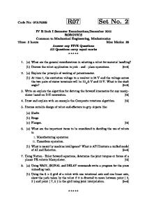
Only time and Normalized FD-SCA have been shown for ease of visibility. As is obvious, the steady state error has descrased as compared to scenario # 1, due to increase in M but, the Normalized FD-SCA converges much faster than SCA. Also the variance of MSE of Normalized FD-SCA is less than SCA. This is because the algorithm works on a block of data and error is calculated for the whole block at once which results is averaging of noise and hence less MSE.
Figure 5-7 Performance evaluation for FD-SCA for Scenario # 3
41
Generated by Foxit PDF Creator © Foxit Software http://www.foxitsoftware.com For evaluation only.
Scenario # 3 & 4: Figure 5.7 shows the results for “chan 11” with M = 16 and for M = 128, the results are shown in figure 5.8.
Figure 5-8 Performance evaluation for FD-SCA for Scenario # 4
Again, The Normalized FD-SCA converges much faster than the SCA. These simulation results show the superiority of performance of Normalized FD-SCA over time domain SCA. Scenario # 5: For 16 QAM, the results are shown below
Figure 5-9 Performance evaluation for FD-SCA for Scenario # 5
42
Generated by Foxit PDF Creator © Foxit Software http://www.foxitsoftware.com For evaluation only.
The gain in performance is more in the case of 16 QAM than in QPSK. As shown in the figure above Normalized FD-SCA takes almost 20,000 less symbols to converge to the steady state. Also the variance of MSE is less than the time domain. Below are the results for scenario # 6.
Figure 5-10 Performance evaluation for FD-SCA for Scenario # 6
5.4.2 Simulation Results for FD-MSCA Simulation results for MSCA will now be provided. As MSCA already includes the CME term for enhancement of convergence rate, the improvement in convergence provided by FD-MSCA is not as pronounced as in FD-SCA. The comparison again, will be performed in different scenario summarized as below.
Scenario
SNR
Modulation
Channel Model
Equalizer Length = Block size
Step Size β
Β applied after samples
µ
1.
30
QPSK
Chan 11
128
0.5* 10 -4
10/Π
5000
2.
30
QPSK
Chan 11
128
0.5* 10 -4
10/Π
0
43
Generated by Foxit PDF Creator © Foxit Software http://www.foxitsoftware.com For evaluation only.
3.
30
QPSK
Voice band
16
0.5* 10 -4
5/ Π
0
4.
30
16QAM
Voice band
16
0.1* 10 -5
10/Π
0
5.
30
16 QAM
Chan 11
16
0.1* 10 -5
10/Π
0
Table 5-2: Simulation parameters for FD-MSCA
Scenario # 1: Figure 5.11 shows the results for scenario # 1. As the CME term is applied after 5000 samples, the MSE curves show a sharp decrease after 5000 samples. FD-MSCA performs same as SCA while the normalized FD-MSCA converges faster than MSCA.
Figure 5-11 Performance evaluation for FD-MSCA for Scenario # 1
Scenario # 2: If the CME term is applied from the start, the convergence speed of all algorithms is further improved. But the Normalized FD-MSCA still converges faster.
44
Generated by Foxit PDF Creator © Foxit Software http://www.foxitsoftware.com For evaluation only.
Figure 5-12 Performance evaluation for FD-MSCA for Scenario # 2
Scenario # 3: The results for the voice band communication channel mentioned in chapter 2 will now be presented. As the impulse response contains only 7 taps, even a 16 length equalizer achieves a very low MSE as compared to previous scenarios.
Figure 5-13 Performance evaluation for FD-MSCA for Scenario # 3
45
Generated by Foxit PDF Creator © Foxit Software http://www.foxitsoftware.com For evaluation only.
Scenario # 4: Consistent with the results for FD-SCA, the improvement in convergence in the case of 16 QAM is higher than QPSK in FD-MSCA also. Figure below shows the results.
Figure 5-14 Performance evaluation for FD-MSCA for Scenario # 4
Scenario # 5: The results for “chan11” for 16 QAM will now be presented. As shown in the figures the improvement in convergence is more than scenario # 2, which is for QPSK.
Figure 5-15 Performance evaluation for FD-MSCA for Scenario # 5
46
Generated by Foxit PDF Creator © Foxit Software http://www.foxitsoftware.com For evaluation only.
The FD-SCA and FD-MSCA deal with frequency domain implementations of SCA and MSCA, respectively. Through simulation results for different channels and different modulations schemes, it is evident that FD-SCA and FD-MSCA performs same as SCA and MSCA in terms of residual ISI and MSE but with much less computational complexity. On the other hand, Normalized FD-SCA and FD-MSCA outperform SCA and MSCA both in term of computational complexity and convergence. The improvement in convergence is more in FD-SCA as compared to FD-MSCA because MSCA already has improved convergence due to CME term and there is little margin to perform. Also, there is more improvement in convergence as higher order constellations are used like 16QAM. Now, the hardware implementation of FD-SCA will be discussed in the next chapter.
47
Generated by Foxit PDF Creator © Foxit Software http://www.foxitsoftware.com For evaluation only.
Chapter 6
Hardware Implementation of FD-SCA
In this chapter, implementation of the proposed FD-SCA algorithm on FPGA will be discussed. First, the fixed point implementation of FD-SCA on MATLAB will be presented and then the design will be transferred to Xilinx ISE 9.2.
6.1 Fixed Point Implementation in MATLAB The algorithm discussed in the previous chapter was simulated on MALTAB using its default 64bit floating point precision. In order to implement the algorithm on Hardware like FPGA, fixed point realization of the algorithm is necessary. This is to ensure that minimum possible hardware is utilized provided the degradation in performance is negligible. So, the aim in the fixed point implementation is to determine exactly, the number of bits required for each component of the algorithm. This fixed point implementation is inspired by [21] which discusses the implementation of Intellectual Property (IP) Core for CMA, MMA and its variants. In this thesis, fixed point FD-SCA for QPSK and Normalized 16 QAM has been implemented. For this purpose, the fixed point environment of MATLAB has been used, which allows the user to assign custom binary bit precision to every variable. It also allows allocating the precision of results of multiplication. The precision of a variable or constant is specified in terms of Integer and Fractional Word length. For example, in communication systems, usually the input / output of the system are in 16/14 precision. It means that the total number of binary bits used to represent this number (Word Length) is 16 out of which 14 are fractional bits and the remaining 2 bits are integer bits. Out of these two bits, one is the sign bit and other is the magnitude bit. So, through fixed point implementation in MATLAB, minimum possible word lengths for each component like the input, output, error and weight vectors are determined.
48
Generated by Foxit PDF Creator © Foxit Software http://www.foxitsoftware.com For evaluation only.
6.1.1 Fixed Point Implementation of FD-SCA FD-SCA was simulated with fixed point environment in MATLAB. The resulting word lengths appropriate word lengths were Input : 16 / 14 Output: 16 / 14 Error: 22/14 Weight Vector 22/14 Fixed point simulations were performed with these word lengths. The results are shown below. “chan 11” was used for simulation at an SNR of 30 dB. The ISI and MSE curves of fixed point FD-SCA almost match with FD-SCA as shown in the figure 6.1 for QPSK and figure 6.2 for 16 QAM.
Figure 6-1 Comparison of fixed point implementation of FD-SCA for QPSK
The results have been averaged over 100 trials. As obvious, there is almost no difference in precision between the two implementations. Similar results were obtained for the other channels used in the thesis. With these but precisions, FD-SCA has been implemented on Xilinx ISE 9.2. 49
Generated by Foxit PDF Creator © Foxit Software http://www.foxitsoftware.com For evaluation only.
Figure 6-2 Comparison of fixed point implementation of FD-SCA for 16 QAM
6.2 FPGA Implementation of FD-SCA FD-SCA with maximum block size i.e. equal to the equalizer length has been implemented on FPGA. The methodology used for implementation is “Algorithmic State Machine” (ASM) [22]. ASM is the graphical representation of the architecture in which the algorithm is divided into different states. At any time, the functionality of the architecture depends on the state in which the algorithm is. ASM of the algorithm was first drawn on paper and the FPGA design followed that ASM. ASM was made keeping in mind the constraints of the hardware, which will be discussed shortly. First, the modules or IP cores of the FPGA used in the design will be discussed along with their constraints and implications. Then, the ASM for the algorithm will be presented.
6.2.1 Hardware Modules The built in hardware modules or Intellectual property (IP) cores used in the architecture are
50
Generated by Foxit PDF Creator © Foxit Software http://www.foxitsoftware.com For evaluation only.
6.2.1.1
Fast Fourier Transform IP Core
FFT / IFFT IP core “Fast Fourier Transform v 5.0”provided by the Xilinx ISE 9.2 has been used in the hardware implementation. The input output block diagram of the core is shown below. The core can be run in four modes namely “Pipelined Streaming IO” “Radix-4 Burst IO” “Radix-2 Burst IO” and “Radix2 Lite Burst IO”. Pipelined Streaming IO has been used in the implementation. It takes complex data serially on XN_RE and XN_IM ports and gives serial output on XK_RE and XK_IM ports.
Figure 6-3 I/O description of FFT IP core (Taken from FFT IP Core Data Sheet)
‘FWD_INV’ pin controls whether the core calculates the FFT or IFFT. With ‘FWD_INV’ equals 1, FFT is computed and vice versa. ‘EDONE’ port is set to by the core one cycle before the appearance of output on ‘XK_RE’ and ‘XK_IM’ while ‘DONE’ is set along with the output.
51
Generated by Foxit PDF Creator © Foxit Software http://www.foxitsoftware.com For evaluation only.
When the ‘START’ pin is set, the core takes the data appearing on ‘XN_RE’ and ‘XN_IM’ as input after ignoring the first four clock cycles. This means one has to wait for 4 clock cycles before applying logical data on XN_RE and XN_IM. For this purpose a data buffer named as “data_buffer_re” and “data_bugger_im” has been used. We use data_buffer to refer to both the real and imaginary buffers. Each buffer holds three data symbols at a time. The input is pushed from one side of the data_buffer_re (data_buffer_im) and the other side of the buffer is connected to XN_RE (XN_IM). In this way the data entering the buffer appears at the XN_RE (XN_IM) at the fourth positive clock edge as shown in the figure 6.5. The FFT core also takes a certain delay to calculate the output after the application of Input. This delay depends on the FFT size and the word-length of the input. For example, for an FFT size of 16 and word-lengths of 22, it takes 102 clock cycles to generate the output.
6.2.1.2
Multiplier
The multiplier core provided by Xilinx ISE 9.2 has been used for multiplications.
6.3 Description of the Architecture The simplified diagram of the algorithm is shown in the figure 6.4. It will be referred during the explanation of the hardware design. Looking at the block diagram, one infers that five FFT/IFFT modules will be needed for the hardware implementation along with the adders and multipliers. But, only on FFT module has been instantiated, which has been reused for FFT/IFFT computations as explained below. We have divided figure 6.4 into different stages to show the functionality of the implementation. Their implementation has also been shown in figure 6.5 and in the ASM in figure xx.
6.3.1.1
Stage 1
It refers to FFT of the input block. Input is applied to data_buffer which is connected to input of the fft core on the other side as explained earlier. At the same time the weight update is also carried out depending upon the output from Stage 5 i.e. the gradient. The gradient is multiplied with µ and added
52
Generated by Foxit PDF Creator © Foxit Software http://www.foxitsoftware.com For evaluation only.
to the weights. This operation requires two multipliers. At the first iteration, this output is zero, so the weights remain the same.
6.3.1.2
Stage 2
When the output of FFT of input data appears on XK_RE and XK_IM, its multiplication with updated weights is carried out. As it is complex multiplication it requires 4 multiplier. Also these samples are stores in “store_re” and “store_im” to use during stage 4 in the future. FWD_INV is set to 0. As the FFT core gives the output serially, the multiplication is carried out sample by sample as it appears on the core output and at the same time, it is applied to data_buffer for IFFT operation. As shown in figure 6.5, the data_buffer_re and data_buffer_im are connected to multiple inputs. The stage determines which input is connected to data_buffer_re and data_buffer_im at that time.
6.3.1.3
Stage 3
FWD_INV is set to 1. When the output of the IFFT appears, first M samples are discarded. The error is calculated for the last M samples. The error calculation consumes 4 multipliers. These M error samples are then appended with M zeros and again applied to data_buffer_re and data_buffer_im to calculate FFT of the error samples as indicated in figure 6.4.
6.3.1.4
Stage 4
The output of the FFT to error samples is multiplied with corresponding samples stored in “store_re” and “store_im”. This multiplication again requires 4 multipliers as it is complex multiplication. The result of multiplication is applied to data_buffer for IFFT calculation.
6.3.1.5
Stage 5
First M samples of the output of IFFT are applied to data_buffer proceeded by M zeros for calculating the FFT. The output of the stage 5 i.e. the gradient is then used in stage 1 in the next iteration. The ASM of the algorithm is shown in figure 6.6
53
Generated by Foxit PDF Creator © Foxit Software http://www.foxitsoftware.com For evaluation only.
Figure 6-4 Bock Diagram for FD-SCA with B = M
54
Generated by Foxit PDF Creator © Foxit Software http://www.foxitsoftware.com For evaluation only.
data_buffer_re
data_buffer_im
Input_re
Input_im
connected to XN_IM
connected to XN_RE
FFT / IFFT
Stage 5 Delete last M samples Append M zeros
Stage 4 Error in Frequency is multiplied with Conjugate of output of stage 1
3Stage 2 Delete first M samples Calculate Error for the last M samples Appends the M zeros
Stage 2 Multiplication with Weights
Figure 6-5 Use of FFT core and data_buffer
The algorithmic state machine of the whole algorithm is shown below.
55
Generated by Foxit PDF Creator © Foxit Software http://www.foxitsoftware.com For evaluation only.
S0 Wait until reset = 0 and control = 1 Output_valid = 0 Fwd_inv = 1
Init = 1 initializes all variables to zero and weight vector to zero except the centre unitary spike
init = 0 start =0
control = 0 reset = 0 Start applying the inout data to FFT core start = 0 data_buffer_re = input_re data_buffer_im = input_im
S1 1. Apply the input data to FFT Update the weights by setting Weight_update = 1
output_valid = 0 start = 0
Count < fft_size-1
Weight_update = 1
Shift_new = 1
Shift_zero = 1
count_inc = 1
count < fft_size+2 S2 Wait until the FFT core gives the output
output_valid = 0 count_reset = 1
edone = 1
start = 1
output_valid = 0 start = 0 store_re = xk_re store_im = xk_m
start = 0
S3 1.Store the ouput in store_re & store_im, 2. multiply the weight vector with the output 3. set fwd_inv = 0 4. Apply the result of multiplication to FFT core
Figure 6-6 The Algorithmic State Machine
56
Generated by Foxit PDF Creator © Foxit Software http://www.foxitsoftware.com For evaluation only.
Yes
count < fft_size -1
No
shift_new = 1
shift_zero = 1
count_inc = 1 Data_buffer_re = p_re Data_buffer_im = p_im
count < fft_size +2 S4 Wait until the IFFT computation is completed output_valid = 0 fwd_inv = 1 count_reset = 1
edone = 1
No
start = 0
Yes start = 1 address_dec = 1 S5 Delete first M samples
output_gvalid = 0 start = 0
count < half -1
Yes
shift_zero = 1 Count_inc = 1
No S6 1.Compute error for the last M samples and give the error samples as input to FFT 2. insert M zeros after the M error samples
count_reset = 1
output_valid = 0 start = 0
Figure 6.6: The Algorithmic State Machine (continued)
57
Generated by Foxit PDF Creator © Foxit Software http://www.foxitsoftware.com For evaluation only.
Yes
count < half -1
No
shift_new = 1 output_valid = 1
shift_zero = 1 output_valid = 0
output_re = xk_re output_im = xk_im R_sub_re = xk_re2 – R R_sub_im = xk_im2 - R
count < half + 2
xk_re[in_data_width - 1] = 0
xk_im[in_data_width - 1] = 0
Yes
Yes abs_xk_re = 0xk_re
abs_xk_re = xk_re
No
E_re = 0
abs_xk_im = xk_im
abs_xk_re >abs_xk_im
count < half + 2
Yes
Yes
E_re = R_sub_re * |xk_re|
E_im = R_sub_im * |xk_im|
abs_xk_im = 0xk_im
No
E_im = 0
count_control = 1 data_buffer_re = e_re data_buffer_im = e_im
output_valid = 0 fwd_inv = 1 count_reset = 1 S7 Wait until the FFT of the error is computed
edone = 1
No
start = 0
Go to S1
Figure 6.6: The Algorithmic State Machine (continued)
58
Generated by Foxit PDF Creator © Foxit Software http://www.foxitsoftware.com For evaluation only.
This chapter discussed the hardware implementation of the algorithm. As it is the first experience of the author with FPGA, this hardware implementation is not the most optimal one. Work is still being carried out on different simplifications and optimizations possible in the architecture.
59
Generated by Foxit PDF Creator © Foxit Software http://www.foxitsoftware.com For evaluation only.
Conclusions and Future Suggestions In this thesis, frequency domain implementation of Square Contour Algorithm has been carried out. The algorithm has been designed, simulated on MATLAB and implemented on FPGA. Improved convergence and reduction in computational complexity resulting from this implementation, calls for frequency domain implementations of the other algorithms as well. Also, the performance of most blind equalization algorithm has not been tested in time selective fading. An analysis to determine the amount of Doppler, the algorithm can withstand without significant degradation in its performance can be an interesting topic of research and the author intends to do this analysis in the near future. Bringing the channel statistical characteristics in the cost function of the equalizer can also bring new dimensions in blind equalization. In certain cases like transmission in the indoor environment, one often has some information about the channel like its maximum delay spread and power delay profile (exponential in most of the cases). This information can be used to find analytical expressions of the autocorrelation matrix of the channel. This matrix can be used in de-correlation of input, as mentioned in chapter 2, to improve the convergence rate. Finally, the extension of the algorithm for MIMO systems can also be a significant contribution.
60
Generated by Foxit PDF Creator © Foxit Software http://www.foxitsoftware.com For evaluation only.
References [1] A.H. Syed, “Fundamentals of Adaptive Filtering”, Published by Wiley-IEEE, 2003. [2] Y. Sato, “A Method of Self-Recovering Equalization for Multilevel Amplitude-Modulation Systems”, IEEE transactions on Communications 1975. [3] D. Tse, P. Viswanath, “Fundamentals of Wireless Communications”, Published by Cambridge University Press, 2005. (Page 29 - 35). [4] T. Thaiupathump, L. He and S. A. Kassam, “Square contour algorithm for blind equalization of QAM signals” Elsevier DSP Journal 2006. Available on www.scinceditrect.com. doi:10.1016/16/j. sigpro.2006.02.035 [5] T.S. Rappaport, “Wireless Communications: Principles and Practice”, Prentice Hall, 2002. [6] D.N. Godard, “Self-Recovering Equalization and Carrier Tracking in Two-Dimensional Data Communication Systems”, IEEE Transaction on Communications, Nov 1980. [7] K. Nam Oh et.al., “Modified constant modulus algorithm blind equalization and carrier phase recovery algorithm”, IEEE International Conference on Communications, 1995. [8] J. Yang, J.J. Werner, G.A. Dumont, “The multimodulus blind equalization and its generalized algorithms”, IEEE Journal on Selected Areas in Communications, June 2002. [9] D. N. Godard, P. E. Thirion, “Method and device for training an adaptive equalizer by means of an unknown data signal in a QAM transmission system”, U.S. Patent 4 227 152, Oct. 7, 1980. [10] L. He, M. Amin, C. Reed, R. Malkemes, “A hybrid adaptive blind equalization algorithm for QAM signals in wireless communications”, IEEE Transaction in Signal Processing. 52 (7) (July 2004) 2058–2069. [11] A.V. Oppenheim, R.W. Schafer, “Discrete-Time Signal Processing”, Published by Prentice Hall Inc. 1999.
61
Generated by Foxit PDF Creator © Foxit Software http://www.foxitsoftware.com For evaluation only.
[12] D. Falconer, S.L. Ariyavisitakul, A. Benyamin-Seeyar, B. Eidson, “Frequency domain equalization for single-carrier broadband wireless systems”, IEEE Communications Magazine, Volume 40, Issue 4, April 2002. [13] J. Shynk, “Frequency-Domain and Multi rate adaptive filtering”, IEEE Signal Processing Magazine, 1992. [14] J. Shynk, ”Frequency-domain implementations of the constant modulus algorithm”, 23rd Asilomer conference on signals, systems and computers,1989. [15] H. H. Dam et.al. “Frequency domain constant modulus algorithm for broadband wireless systems”, IEE GLOBECOM 2003. [16] Y. G. Yang, N. Ik Cho and S. Uk Lee, “Fast Blind Equalization by Using Frequency Domain Constant Modulus Algorithm”, Proceedings of the 38th Midwest Symposium on Circuits and Systems, 1995. [17] Y. G. Yang, C. H. Park and J. Song, “Fast Constant Modulus Algorithm in the DFT domain”, IEEE Radio and Wireless Conference, 2004. [18] G.H. Im, D. D. Harman, G. Huang, A. V. Mandzik, M.-H. Nguyen, and J. J. Werner, “51.84 Mb/s 16CAP ATM-LN standard,” IEEE Journal on Selected Areas in Communication, vol. 13, pp. 620–632, May 1995. [19] G.-H. Im and J. J. Werner, “Bandwidth-efficient digital transmission over unshielded twisted pair wiring,” IEEE Journal on Selected Areas in Communication, vol. 13, pp. 1643–1655, Dec. 1995. [20] D. D. Harman, G. Huang, G.-H. Im, M.-H. Nguyen, J. J.Werner, and M. K. Wong, “Local distribution for IMIV,” IEEE Multimedia, vol. 2, pp. 14–23, Fall 1995. [21] K. Banovi´c, M. A. S. Khalid and E. Abdel-Raheem, “A Configurable Fractionally-Spaced Blind Adaptive Equalizer for QAM Demodulators”, Elsevier Digital Signal Processing Volume 17, Issue 6, November 2007, Pages 1071-1088. [22] S. Brown, Z. Vrsaniec, “Fundamentals of Digital Logic with Verilog Design” McGraw Hill Publishers
62