Clustering Based Active Learning for Evolving Data Streams ˇ Dino Ienco1 , Albert Bifet2 , Indr˙e Zliobait˙ e3 and Bernhard Pfahringer4 1

3

Irstea, UMR TETIS, Montpellier, France LIRMM, Montpellier, France [email protected] 2 Yahoo! Research Barcelona, Catalonia, Spain [email protected] Aalto University and Helsinki Institute for Information Technology, Finland [email protected] 4 University of Waikato, Hamilton, New Zealand [email protected]

Abstract. Data labeling is an expensive and time-consuming task. Choosing which labels to use is increasingly becoming important. In the active learning setting, a classifier is trained by asking for labels for only a small fraction of all instances. While many works exist that deal with this issue in non-streaming scenarios, few works exist in the data stream setting. In this paper we propose a new active learning approach for evolving data streams based on a pre-clustering step, for selecting the most informative instances for labeling. We consider a batch incremental setting: when a new batch arrives, first we cluster the examples, and then, we select the best instances to train the learner. The clustering approach allows to cover the whole data space avoiding to oversample examples from only few areas. We compare our method w.r.t. state of the art active learning strategies over real datasets. The results highlight the improvement in performance of our proposal. Experiments on parameter sensitivity are also reported.

1

Introduction

Today, large amounts of data are being generated continuously, and we are creating more data every two days, than all the data we created before 2003 [15]. Data streams pose new serious challenges to the data analysis community. To learn supervised models, we need to obtain true labels from the instances of the streams . This labeling phase is usually an expensive and tedious task for domain experts. Consider, for example, textual news arriving as a data stream. The goal is to predict if a news item will interest a given user at a given time. The interests of the user may change over time. To obtain training data, news need to be labeled as interesting or not interesting. This requires human labor. For instance, Amazon Mechanical Turk5 provides a marketplace for intelligent human labeling. 5

https://www.mturk.com

Labeling can also be costly because it requires expensive, intrusive or destructive laboratory test. Consider a production process in a chemical plant where the goal is to predict the quality of production output. The relationship between input and output quality might change over time due to constant manual tuning, complementary ingredients or replacement of physical sensors. In order to know the quality of the output (the true label) a laboratory test needs to be performed which is costly. Under such conditions it may be unreasonable to require true labels for all incoming instances. A way to alleviate this issue is to ask for labels, over time, for only a small and reasonable portion of the data. The main question then is: How can we select a good subset of instances for learning a model? Such a learning scenario is referred to as active learning. Active learning studies how to label selectively instead of asking for all true labels. It has been extensively studied in pool-based [13] and online settings [5]. In pool-based settings the decision concerning which instances to label is made by ranking all historical instances (e.g. according to uncertainty) while in online active learning each incoming instance is compared to a threshold (e.g. an uncertainty threshold) and the system asks for the true label if the threshold is exceeded. The main difference between online active learning and active learning in data streams is in expectations around changes. In data streams the relationship between the input data and the label may change (concept drift) and these changes can happen anywhere in the instance space while online learning assumes a stationary relationship between examples and their labels. As mentioned before, concept drifts in streams can happen anywhere in the data. To cope with this issue previous works exploit randomization strategies to span the whole instance space [24]. We propose a clustering based approach ACLStream (Active Clustering Learning for Data Streams)to better deal with possible drifts. More specifically, when a batch of instances arrives, we first partition these instances using a clustering algorithm. Then we query examples for labeling by combining geometrical information (supplied by the clustering) and the maximum a posteriori probability of the model learnt from all the labelled examples from previous batches of data. Once the query labels are obtained, the data stream classifier is updated and it is ready to classify new incoming data. The proposed strategy allows to selectively sample a subset of well distributed instances in the data space. We demonstrate that the selected examples summarize the stream sufficiently for learning an evolving classification model. The remainder of this paper is organized as follows. Section 2 briefly explores the state of the art in active learning for data streams and makes some connections with semi-supervised learning in data streams. The proposed methodology is presented in Section 3. In Section 4 we present experimental results for a number of real world datasets and we also supply a sensitivity analysis of the essential parameters of the approach. Finally, Section 5 concludes the study.

2

Related work

Online active learning has been the subject of a number of studies, where the data distribution is assumed to be static [2, 5, 9, 20]. The goal is to learn one accurate model with minimum labeling effort. In contrast, in the evolving data streams setting, which is the subject of our study, the goal is to continuously update a model over time so that accuracy is maintained as the data distribution is changing. The problem of label availability in evolving data streams has been the subject of several recent studies [6, 10, 12, 17, 22, 24] that fall into three main groups. The first group of works uses semi-supervised learning approaches to label some of the unlabeled data automatically [12, 17, 22], which can only work under the assumption that the class conditional distribution does not change (no concept drift). Semi-supervised learning approaches are conceptually different from the active learning approaches, that are the subject of our study, since the former can only handle changes in the input data distribution, changes in the relation between the input data and the target label cannot be spotted without querying an external oracle as is done in active learning. The second group of works process data in batches implicitly or explicitly assuming that data is stationary within batches [6, 10, 14, 16]. Such approaches require an external mechanism to handle concept drift. Lindstrom et al. [14] use uncertainty sampling to label the most representative instances within each new batch. They do not explicitly detect changes, instead they use a sliding window approach, which discards the oldest instances. Masud et al. [16] use uncertainty sampling within a batch to request labels. In addition, they use the unlabeled instances with their predicted labels for training (semi-supervised learning approach). A few works integrate active learning and change detection [6, 10] in the sense that they first detect change and only if change is detected do they ask for representative true labels using offline active learning strategies designed for stationary data. In this scenario drift handling and active learning can be considered as two mechanisms operating in parallel, but doing so independently. This is the main difference between this scenario and the last one, which combines the two mechanisms more closely together. Finally, the third group of works use randomization to capture possible changes in the class conditional distribution [4, 23, 24]. Cesa-Bianchi et al [4] develop an online active learning method for a perceptron based on selective sampling using a variable labeling threshold b/(b + |p|), where b is a parameter and p is the prediction of the perceptron. The threshold itself is based on certainty expectations, while the labels are queried at random. This mechanism could allow adaptation to changes, although they did not explicitly consider concept drift. Zhu et al. [23] build a classifier on a small portion of data within a batch at random and use uncertainty sampling to label more instances within this batch. A new classifier in each batch is needed to take into account concept drift. Zliobaite et al. [24] operate in the pure online setting without batches, where they combine stationary online active learning with randomization over the instance space. Our study moves a step further from just employing random-

ization over the instances to capture a potential concept drift. We use stratified sampling over the instance space instead, where the strata are determined using a clustering mechanism. The idea of pre-clustering has been considered for active learning in the stationary setting [18]. The selection criterion gives priority to two types of samples: samples close to the classification boundary and samples which are cluster representatives. This way the prior data distribution can be taken into account when making labeling decisions, which has been shown to work well empirically and theoretically for certain data distributions. Employing clustering is conceptually similar to our approach, however, the motivation behind doing that in our approach is different. We mainly aim at tracking concept drift using this mechanism.

3

Setting and Methods

In this section we describe our new algorithm ACLStream (Active Clustering Learning for Data Streams). We suppose that our incoming data stream is divided into batches. Each batch St is associated with the arrival time denoted by the index t: S = {S1 , S2 , ..., Sn , ...}. This scenario is general enough to model arbitrary real-world data streams. Note that even in the case of a fully incremental scenario, we can still build batches by employing a buffer based procedure to collect examples. Given a data stream S and a budget b we want to learn a classifier cl with only b% of the instances in the stream. How to select the instances to query is challenging for any active learning strategy. As we are working in a batch incremental scenario, this means that if the value of b is 0.2 we can select 20% of the labels for each batch St . The proposed strategy is based on the clustering of instances in a batch. To select a query point, first we choose a cluster and then we select as query one of the instances belonging to that cluster. The use of clusters helps the selection strategy to sample queries from different, but still reasonably densely populated parts of the instance space. In this way we hope to improve coverage for the different classes of the problem and to overcome possible concept drift that can appear anywhere in the data space. Once the clustering is produced we need to determine (i) which are the most useful clusters to select, and (ii) given a cluster, which are the most useful instances inside this specific cluster. For both cases we will define a ranking for all respective objects, clusters or instances. Thus we implement a two step procedure. As a Macro Step, we need to define how to produce a suitable ranking of clusters and then, as a Micro Step, we need to define how to rank the instances inside each cluster in order to retrieve the most informative instances for labeling first. The use of clustering, to select query instances, allows covering the whole data space, albeit in a more focused manner than purely random sampling. Points from all areas of the instance space may be sampled, which is a welcome property in a data stream scenario in which concept drifts can appear anywhere. Contrary to randomized strategies [24], that also try to cover the whole data space, ACLStream is guided by the partitioning of the space induced by the

clustering algorithm. One of the advantages is higher robustness with regard to outliers, where purely random sampling might waste valuable labeling resources. 3.1

Macro Step: Evaluating the Importance of a Cluster

After clustering of a batch is finished, we evaluate the quality of each partition employing the classifier cl which was trained on all previously labeled data. We classify all the instances of the batch St without taking into account the clustering solution. After the classification step, we compute, separately for each cluster, a distribution vector w.r.t. the class values. This means that each cluster C∗ will be associated with a vector of length equals to the number of classes. We indicate this vector as VC∗ . Each cell of the vector contains the number of instances in the cluster, for which the classifier predicts that specific class value. Intuitively, if the vector is balanced – all the class values are equally probable – that cluster covers a more difficult part of the data space to classify in comparison to a cluster with a very skewed distribution, in which there is a clear predominant class value. Starting from this intuition, we introduce a function to quantify the homogeneity of the predicted class distribution in a cluster. In particular, the proposed measure returns values closer to 0 when class values are equally probable while it returns 1 when the cluster is homogeneous w.r.t. the predicted class values. The homogeneity function is defined as follows: P|VC∗ | P|VC∗ | homogeneity(C∗ ) =

|VC∗ [i] − VC∗ [j]| size(C∗ ) ∗ (|VC∗ | − 1)

i=0

j=i+1

(1)

where size(C∗ ) is the number of instances in the cluster C∗ . The homogeneity function is bounded between 0 and 1. The numerator evaluates the variation of the prediction among the different class values to evaluate how far is from a completely equiprobable situation. The numerator is then normalized by the extreme case in which we assume that all the examples, in the cluster, are assigned to the same class value. Clusters are sorted in increasing value of their homogeneity, from perfectly balanced to fully homogeneous. 3.2

Micro Step: Instance certainty inside a cluster

In order to quantify the importance or certainty of each instance, inside each cluster, we combine two different factors. One is based on the centrality of the instance w.r.t. its cluster centroid while the second one exploits the classifier cl. To compute the centrality of an instance xi w.r.t. its cluster C∗ we simply use the Euclidean distance between xi and the centroid of C∗ (centroid(C∗ )). We refer to this quantity using the notation d(xi , C∗ ) without explicitly indicating the use of centroid(C∗ ) to simplify the notation. The second factor is computed by the classifier. We use the maximum a posteriori probability of the classifier for the particular instance xi . The maximum a posteriori probability is the maximum among all the class probabilities predicted for xi . We indicate the maximum a

posteriori using the notation M APcl (xi ). Given a cluster C∗ and an instance xi belonging to that cluster, the centralized certainty of the instance is supplied by the following formula: certainty(xi ) = M APcl (xi ) ∗ d(xi , C∗ )

(2)

Intuitively we want to select instances i) for which the decision of the classifier is less clear and ii) which are good representatives, or exemplars, for the area covered by the cluster. To do this we combine the M APcl (xi ) that represents point i) and d(xi , C∗ ) corresponding to point ii) by multiplication, and name the resulting quantity the certainty of xi . Then, for each cluster, all instances are sorted by increasing values of certainty. Therefore the most uncertain instances will be selected first for labeling. 3.3

ACLStream strategy

Given a batch of instances St and a budget b, our solution uses clustering to select a fraction (b) of instances from batch St that are deemed the most informative for training a stream classifier. cl first classifies the incoming instances, then we cluster the elements in St , obtaining a partition C = {C1 , ..., Ck }. After clustering, we apply our sampling strategy. First we perform the macro-step that ranks the clusters in C according to the homogeneity function defined in Equation 1. After that, for each cluster, we perform the micro-step which ranks the instances according to their certainty (Equation 2). The returned result is a set X of instances selected for labeling. The procedure is summarized in Algorithm 1. Our solution can also be adopted to work in a one-by-one classification scenario. Using a buffer that collects batches of instances, the classifier continuously classifies examples until the batch is full. At that point, we can interrupt the classification process, select query points through the active learning strategy, update the classifier and reset the buffer to restart collecting examples. As a clustering algorithm we employ the standard K-Means algorithm [21]. Any kind of clustering algorithm could be used to perform this step. The use of K-Means is motivated by its time complexity, which is linear w.r.t. the size of the batch, and by the fact that it is generally used as universal baseline in clustering. Future work will investigate the utility of alternative clusterers. Once the partition is available, we rank the clusters w.r.t. their homogeneity (see Formula 1). Clusters at the top of the ranking are the most balanced ones in terms of their class distributions. Therefore they also represent areas of the instance space over which the classifier is less confident. This ranking is stored in a ranked list Lc . Then, for each cluster c of Lc we rank their instances. This ranking is performed employing Formula 2. At this point we have quantified the usefulness of both clusters and instances. To select instances for labelling, we start from the top ranked cluster and we select and remove the first instance. Then, iteratively, we select one instance from every other cluster in order to explicitly cover all the different areas of the data space. If the budget exceeds

Algorithm 1 ACLStream(St , cl, b, k) Require: St : batch of instances Require: cl: classifier Require: b: budget Require: k: number of clusters 1: X = ∅ 2: C = clustering(St ,k) 3: Lc = rankClusters(C, cl) according to homogeneity (eq. 1) 4: for all c ∈ Lc do 5: rankExamples(c, cl) according to certainty (eq. 2) 6: end for 7: for i = 1 → b × size(St ) do 8: X = X ∪ dequeue(Lc [i % k]) 9: end for 10: return X

the number of clusters, we restart to sample instances again starting from the top of the cluster ranking. If the budget is low and the number of instances to sample is smaller than the number of clusters we only consider clusters in the top of Lc . 3.4

General Classification Schema

Algorithm 2 summarizes the general classification schema. The Main loop simulates the streaming process collecting batches of data. Once a batch is collected, the data is classified and then used as input for the proposed active learning strategy that returns the set of selected query points. The active learning strategy is realized through Algorithm 1. To evaluate classifier performance we adopt the prequential schema. The evaluation through the prequential setting involves two steps: i) classify an instance, and ii) use the same instance to train the learner. To implement this strategy, first we test all the instances in the batch with the classifier cl. Second, we select examples for labeling using ACLStream. In this way we respect the constraints imposed by our setting. Function askLabel(xj ) simulates the user in the labeling phase. At the end, the classifier cl is trained over the set X of labeled data. The process continues until the end of the data stream is reached.

4

Experiments

In this section we evaluate the performance and the quality of the proposed ACLStream. We compare our algorithm with three other methods that are explicitly designed for active learning over data streams. We use the prequential evaluation procedure: each time an instance arrives, we first test the algorithm on it, and then we decide on whether pay the cost for labeling it and subsequently use it as an input for updating the classifier.

Algorithm 2 Active Learning Process(S, b, k) Require: S: stream of instances Require: b: budget Require: k: number of clusters 1: Init classifier cl 2: while hasMoreInstances(S) do 3: St = extractNextBatch(S) 4: for all xj ∈ St do 5: test(cl,xj ) 6: end for 7: X = ACLStream(St ,cl,b,k) 8: for all xj ∈ X do 9: yj = askLabel(xj ) 10: train(cl,xj ,yj ) 11: end for 12: end while

The first method is a baseline approach, also used in [24], that randomly chooses examples for labeling. We call this method Random. The second method, also proposed in [24], uses a randomized variable uncertainty strategy that combines the randomization with maximum a posteriori probability and an adaptive method to avoid consuming too much of the budget when a consecutive run of easy instances is encountered. We call this approach Rand Unc. The last competitor is an ensemble approach [23] that uses a maximum variance principle. Given a set of classifiers, in a batch incremental scenario, the instances to label are the ones over which the classifiers disagree the most. In the original work, given a batch, the authors propose to first select the instances to label and then classify the remain instances in the batch. To have a fair comparison with the other approaches we wait until the end of the batch before executing active learning. This way the model will be trained to classify the instances of the next batch. We call this classifier MVC (Maximum Variance Classifier). Using this set up i) we ensure that the budget constraints are always respected during the stream process, ii) the comparison is fair w.r.t. our approach and the other two competitors that suppose a full incremental scenario, and iii) we respect prequential learning schema. For all methods a warm-up step is introduced. In detail, the first 500 instances of each dataset are all labeled and used to train the initial model used by the specific approach. Evaluation only starts after this warm-up step. All the methods need a classification algorithm as a base block to perform the classification and to produce the maximum a posteriori probability. For this reason for our approach, for the Random and for the Rand Unc strategies we use the classifier proposed in [7]. This classifier is able to adapt itself to drift situations: when the accuracy of the classifier begins to decrease a new classifier is built and trained with new incoming instances. For MVC we use the C4.5 algorithm [19] as suggested in the original paper. Always following the original paper we use a window size of 1 000 instances for MVC

as that size obtains best results, while for ACLStream we employ a window size of 100 instances. The default number of clusters is 5. As our approach uses a nondeterministic algorithm to perform the clustering, each result for ACLStream is averaged over 30 runs. All our experiments are performed using the MOA data stream software suite [3]. MOA is an open source software framework in Java designed specifically for data stream mining. 4.1

Datasets

To evaluate all the algorithms we use five real world “datasets: Electricity, Cover Type, Airlines, Poker, KDD99. Electricity data [8] is a popular benchmark in evaluating streaming classifiers. The task is to predict the rise or fall of electricity prices (demand) in New South Wales (Australia), given recent consumption and prices in the same and neighboring regions. Cover Type data [1] is also often used as a benchmark for evaluating stream classifiers. The task is to predict forest cover types or types of vegetation from cartographic variables. Inspired by [11] we constructed an Airlines dataset using the raw data from US flight control. The task is to predict whether a given flight will be delayed, given the information of the scheduled departure. The Poker dataset represents all the possible combination of cards in one hand with the corresponding score as the class value. This results in a big dataset with more than 800k instances. The last dataset, KDD99, is commonly used as a benchmark anomaly detection task but recently it has also been employed as a dataset for testing data stream algorithms [17]. One of the big problems with this dataset is the big amount of redundancy among instances. To solve this problem we use the cleaned version named NSL-KDD6 . To build the final dataset we join both training and test data. A summary of the datasets’ characteristics is reported in Table 1. We observe that this collection of datasets contains both binary and multi-class classification problems, datasets with different numbers of instances (varying between 42k to 829k) and different numbers of features (from 7 to 54). For analysis purposes, we also introduce one more dataset, named Cover Type Sorted, in which the instances of the Cover Type dataset are reordered w.r.t. the attribute elevation. Due to the nature of the underlying problem, sorting the instances by the elevation attribute induces a natural gradual drift on the class distribution, because at higher elevation some types of vegetation disappear while other types of vegetation appear gracefully. We think that this final set of six datasets is a good benchmark for evaluating the performance of our approach, ACLStream, w.r.t. state of the art methods. 4.2

Analysis of Classification Accuracies

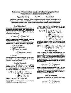
The final accuracy results are reported in Figure 1. In this experiment we evaluate the different methods, over the different datasets, varying the budget percentage. We start with a budget percentage of 0.03 and go up to a percentage of 6

http://nsl.cs.unb.ca/NSL-KDD/

Dataset n. of Instances n. of Features n. of Classes Airlines 539 383 7 2 Electricity 45 312 8 2 Cover Type 581 012 54 7 Poker 829 201 10 10 KDD99 148 517 41 2 Table 1. Dataset characteristics

0.3. Obviously, to evaluate the results we need to take into account both budget size and accuracy. We can observe that, except for KDD99 dataset, ACLStream outperforms the other methods for low budgets, less than 0.15, while for bigger budgets the performances are either better as well, or at least comparable. For the case of KDD99 the performances of Random, Rand Unc and ACLStream are very close to each other and the difference is smaller than 1.5 percentage points of accuracy. Another useful feature of our new method is its stability. As we can see from the graphs, ACLStream always remains stable varying the budget percentage while this is not the case for all the other methods. This behaviour is clearly present for the Cover Type dataset. In this case the Rand Unc strategy is very unstable and small changes of the budget (from 0.15 to 0.25) induce a big change (ten points of accuracy) in the final performance. Also the Random strategy is much more unstable than our proposed method. Another general conclusion we can draw regards MVC, which always obtains low accuracy performance when compared to all the other methods. To wrap up all the findings from this experiment, we can claim that ACLStream works well for very low budget percentages, which is a very important and desirable feature for any active learning strategy. This is particularly important in the data stream domain, in which data arrives continuously and time-consuming operations, such as data labeling, need to be minimized. On the other hand, due to its stability, ACLStream small budget results are very similar to ones obtained with higher budget. This observation implies that the active learning strategy based on our clustering approach is especially effective for small budgets. 4.3

Influence of the Number of Clusters

We evaluate how the number of clusters influences the performance of ACLStream. For this analysis we fix the batch size to 100 as in the general experiment, and we vary the number of clusters from 5 to 25 with a step size of 5. We report results in Figure 2. As we can note, the number of clusters does not affect the general performance of the algorithm, so it is also very stable w.r.t. the setting of this parameter. We can observe that for Airlines, Electricity, KDD99 and Cover Type Sorted datasets the maximum accuracy fluctuation over the different datasets is smaller than 0.8 points of accuracy. For the Cover Type dataset we reach the maximum accuracy gain (1.4 points of accuracy) between k =5 and k =25 when the budget is equal to 0.3. The maximum difference in accuracy (2.5 points of

68.00

80.00

66.00 75.00 Accuracy

Accuracy

64.00 62.00

70.00

60.00 58.00

65.00

56.00 54.00

random rand unc clust k=5,w=100 Maximum Variance Classifier

0

0.05

0.1

0.15 Budget

0.2

0.25

0.3

60.00

random rand unc clust k=5,w=100 Maximum Variance Classifier

0

0.05

0.1

(a)

0.15 Budget

0.2

0.25

0.3

(b)

75.00

85.00

70.00 80.00 Accuracy

Accuracy

65.00

75.00

60.00

70.00 55.00

50.00

random rand unc clust k=5,w=100 Maximum Variance Classifier

0

0.05

0.1

0.15 Budget

0.2

0.25

0.3

65.00

random rand unc clust k=5,w=100 Maximum Variance Classifier

0

0.05

0.1

(c)

0.2

0.25

0.3

(d)

66.00

89.00

64.00

88.00

62.00

87.00

Accuracy

90.00

Accuracy

68.00

60.00

86.00

58.00

85.00

56.00

84.00

54.00 52.00

0.15 Budget

83.00

random rand unc clust k=5,w=100 Maximum Variance Classifier

0

0.05

0.1

0.15 Budget

(e)

0.2

0.25

0.3

82.00

random rand unc clust k=5,w=100 Maximum Variance Classifier

0

0.05

0.1

0.15 Budget

0.2

0.25

0.3

(f)

Fig. 1. Accuracy on a) Airlines b) Cover Type c) Poker d) Electricity e) Cover Type Sorted and f) KDD99

accuracy), among all the experiments, is measured for the Poker dataset for a budget of 0.15. For this dataset, ACLStream with a number of clusters equal to 5 always obtains the best accuracy. Still, even in this case, the performances of different numbers of clusters are very close to each other. The obtained stability w.r.t. the number of clusters underlines that the combination of our macro and micro steps is effective for dealing with the complexity of data streams. Specifically, starting to analyze clusters with low homogeneity, which are clusters covering areas that are ambiguous according to prediction evidence, forces the method to sample examples where labeling information seems

most useful. This is particularly important when the budget size is actually smaller than the total number of clusters. 67.00

78.00 77.50

66.50 77.00 66.00 Accuracy

Accuracy

76.50

65.50

76.00 75.50

65.00 75.00 64.50 64.00

nClust=5 nClust=10 nClust=15 nClust=20 nClust=25

0

0.05

0.1

0.15 Budget

0.2

0.25

nClust=5 nClust=10 nClust=15 nClust=20 nClust=25

74.50 0.3

74.00

0

0.05

0.1

(a)

0.15 Budget

0.2

0.25

0.3

(b)

71.00

82.00

70.00

81.00

69.00 Accuracy

Accuracy

80.00 68.00

79.00

67.00

78.00 66.00

64.00

77.00

nClust=5 nClust=10 nClust=15 nClust=20 nClust=25

65.00 0

0.05

0.1

0.15 Budget

0.2

0.25

0.3

76.00

nClust=5 nClust=10 nClust=15 nClust=20 nClust=25

0

0.05

0.1

(c)

0.15 Budget

0.2

0.25

0.3

(d)

67.00

90.00 89.50

66.50 89.00 66.00 Accuracy

Accuracy

88.50

65.50

88.00 87.50

65.00 87.00 64.50 64.00

nClust=5 nClust=10 nClust=15 nClust=20 nClust=25

0

0.05

0.1

0.15 Budget

0.2

0.25

(e)

nClust=5 nClust=10 nClust=15 nClust=20 nClust=25

86.50 0.3

86.00

0

0.05

0.1

0.15 Budget

0.2

0.25

0.3

(f)

Fig. 2. Accuracy of ACLStream varying the number of clusters from 5 to 25 on a) Airlines b) Cover Type c) Poker d) Electricity e) Cover Type Sorted and f) KDD99

4.4

Influence of the Batch Size

The last set of experiments focuses on the influence of the second parameter: the size of the batches. In particular, we analyze how the size of a batch impacts the final accuracy of ACLStream. For this purpose, we run experiments varying

the size of the batches from 100 to 500 with a step size of 100. We average each result over 30 runs and we set the number of clusters equal to 5. The results are reported in Figure 3. We can observe two distinct behaviors. There is one group of three datasets – Cover Type, Poker and Electricity – for which the batch size influences the final accuracy, and another group comprising the remaining three datasets – Airlines, Cover Type Sorted and KDD99 ) – for which this parameter does not seem to affect the final performance. For the latter group of datasets the fluctuation in accuracy is less than 0.5 points. For the former group of datasets, the ones influenced by the batch size, we can note that in general smaller batches outperform bigger ones. Using small batches forces the learner to adapt faster to possible changes, and to sample instances in a more regular way. This is particularly useful where concept drift happens quickly and frequently. This is the case for the Electricty dataset, where multiple levels of periodicity are present, over 24 hours, over 7 days, and over 4 seasons. Drift can be visually presented by plotting class conditional distributions over time. On the other hand, this is not the case for the Cover Type Sorted dataset, where batch size does not produce significant accuracy changes, as very gradual and smooth concept drift as induced by sorting the instances by the elevation attribute. This gradual drift phenomena can be managed well by all batch sizes evaluated here. To summarize, for ACLStream we can state that small values for batch size are preferable over large ones. Using a small batch size forces the system to sample labels at more regular intervals. Consequently, the learner adapts better and faster in case of fast concept drift, without negatively impacting the performance on datasets where concept drift may be more gradual or not present at all.

5

Conclusions

Building classification models on data streams considering only a limited amount of labeled data is starting to be a common task due to time and cost constraints. In this paper we presented ACLStream, a novel algorithm to perform active learning in a data stream scenario. Our approach exploits a clustering based partitioning of the data space to focus sampling on the potentially most useful examples to label. Clusters are ranked by homogeneity of their predicted class distributions. Instances in each cluster are ranked according to two factors: i) maximum a posteriori classification probability, and ii) geometrical position inside the cluster. Certainty is defined to be the product of these two factors. Instances with low certainty inside a given cluster are preferred, as they represent central points over which the classifier is more uncertain. We assessed the performance of ACLStream over real world datasets and we showed that it outperforms state-of-the-art active learning strategies for data streams. We also empirically studied how our proposal is influenced by the setting of its parameters. As future work we would like to investigate in more detail the use of clustering for active learning in data streams considering alternative clustering algorithms as well as alternative ranking heuristics.

68.00

80.00 78.00

67.50

76.00 67.00 Accuracy

Accuracy

74.00

66.50

72.00

66.00

70.00 68.00

65.50 65.00

BatchSize=100 BatchSize=200 BatchSize=300 BatchSize=400 BatchSize=500

0

0.05

0.1

0.15 Budget

0.2

0.25

BatchSize=100 BatchSize=200 BatchSize=300 BatchSize=400 BatchSize=500

66.00 0.3

0

0.05

0.1

(a)

0.15 Budget

0.2

0.25

0.3

(b)

71.00

82.00

70.00 80.00

69.00 68.00

Accuracy

Accuracy

78.00

67.00 66.00

76.00

65.00 64.00

74.00 BatchSize=100 BatchSize=200 BatchSize=300 BatchSize=400 BatchSize=500

63.00 62.00

0

0.05

0.1

0.15 Budget

0.2

0.25

0.3

72.00

BatchSize=100 BatchSize=200 BatchSize=300 BatchSize=400 BatchSize=500

0

0.05

0.1

(c)

0.2

0.25

0.3

(d)

69.00

89.50

68.00

89.00

67.00

88.50

Accuracy

90.00

Accuracy

70.00

66.00

88.00

65.00

87.50

64.00

87.00 BatchSize=100 BatchSize=200 BatchSize=300 BatchSize=400 BatchSize=500

63.00 62.00

0.15 Budget

0

0.05

0.1

0.15 Budget

(e)

0.2

0.25

BatchSize=100 BatchSize=200 BatchSize=300 BatchSize=400 BatchSize=500

86.50 0.3

86.00

0

0.05

0.1

0.15 Budget

0.2

0.25

0.3

(f)

Fig. 3. Accuracy Results for ACLStream on a) Airlines b) Cover Type c) Poker d) Electricity e) Cover Type Sorted and f) KDD99 varying the batch size from 100 to 500

ˇ Acknowledgements I. Zliobait˙ es research is supported by the Academy of Finland grant 118653 (ALGODAN).

References 1. A. Asuncion and D. Newman. UCI machine learning repository. University of California, Irvine, School of Information and Computer Sciences, 2007. 2. J. Attenberg and F. Provost. Online active inference and learning. In Proc. of the 17th ACM SIGKDD int. conf. on Knowledge discovery and data mining, KDD, pages 186–194, 2011.

3. A. Bifet, G. Holmes, R. Kirkby, and B. Pfahringer. MOA: Massive Online Analysis. J. Mach. Learn. Res., 11(May):1601–1604, 2010. 4. N. Cesa-Bianchi, C. Gentile, and L. Zaniboni. Worst-case analysis of selective sampling for linear classification. J. Mach. Learn. Res., 7:1205–1230, 2006. 5. D. Cohn, l. Atlas, and R. Ladner. Improving generalization with active learning. Machine Learning, 15:201–221, May 1994. 6. W. Fan, Y. Huang, H. Wang, and Ph. Yu. Active mining of data streams. In Proc. of the 4th SIAM Int. Conf. on Data Mining, SDM, pages 457–461, 2004. 7. J. Gama, P. Medas, G. Castillo, and P. Rodrigues. Learning with drift detection. In Proc. of SBIA Brazilian Symp. on Artificial Intelligence, SBIA, pages 286–295, 2004. 8. M. Harries, C. Sammut, and K. Horn. Extracting hidden context. Machine Learning, 32(2):101–126, 1998. 9. D. Helmbold and S. Panizza. Some label efficient learning results. In Proc. of the 10th an. conf. on Computational learning theory, COLT, pages 218–230, 1997. 10. Sh. Huang and Y. Dong. An active learning system for mining time-changing data streams. Intelligent Data Analysis, 11:401–419, 2007. 11. E. Ikonomovska, J. Gama, and S. Dzeroski. Learning model trees from evolving data streams. Data Mining and Knowledge Discovery, 23(1):128–168, 2010. 12. R. Klinkenberg. Using labeled and unlabeled data to learn drifting concepts. In IJCAI Workshop on Learning from Temporal and Spatial Data, pages 16–24, 2001. 13. D. Lewis and W. Gale. A sequential algorithm for training text classifiers. In Proc. of the 17th an. int. ACM SIGIR conf. on Research and development in information retrieval, SIGIR, pages 3–12, 1994. 14. P. Lindstrom, S. J. Delany, and B. MacNamee. Handling concept drift in a text data stream constrained by high labelling cost. In Proc. of the 23rd Int. Florida Artificial Intelligence Research Society Conference, FLAIRS, 2010. 15. J. Manyika, M. Chui, B. Brown, J. Bughin, R. Dobbs, Ch. Roxburgh, and A. Byers. Big data: The next frontier for innovation, competition, and productivity, 2011. 16. M. Masud, J. Gao, L. Khan, J. Han, and B. Thuraisingham. Classification and novel class detection in data streams with active mining. In Proc. of the 14th Pacific-Asia conf. on Advances in Knowledge Discovery and Data Mining, PAKDD, pages 311–324, 2010. 17. M. Masud, C. Woolam, J. Gao, L. Khan, J. Han, K. Hamlen, and N. Oza. Facing the reality of data stream classification: coping with scarcity of labeled data. Knowl. Inf. Syst., 33(1):213–244, 2011. 18. H. Nguyen and A. Smeulders. Active learning using pre-clustering. In Proc. of the 21st int. conf. on Machine learning, ICML, pages 623–630, 2004. 19. R. J. Quinlan. C4.5: Programs for Machine Learning. Morgan Kaufmann Series in Machine Learning. Morgan Kaufmann, 1993. 20. D. Sculley. Online active learning methods for fast label-efficient spam filtering. In Proc. of the 4th Conf. on Email and Anti-Spam, CEAS, 2007. 21. P.N. Tan, M. Steinbach, and V. Kumar. Introduction to Data Mining. AddisonWesley Longman Publishing, 2005. 22. D. Widyantoro and J. Yen. Relevant data expansion for learning concept drift from sparsely labeled data. IEEE Tr. on Know. and Data Eng., 17:401–412, 2005. 23. X. Zhu, P. Zhang, X. Lin, and Y. Shi. Active learning from data streams. In Proc. of the 7th IEEE Int. Conf. on Data Mining, ICDM, pages 757–762, 2007. 24. I. Zliobaite, A. Bifet, B. Pfahringer, and G. Holmes. Active learning with drifting streaming data. IEEE Trans. on Neural Networks and Learning Systems, page in press, 2013.