MINI PROJECT II
ARTIFICIAL SPECIATION AND AUTOMATIC MODULARISATION
by Vineet Khare (ID 462534)
Project Supervisor: Prof. Xin Yao
A report submitted in partial fulfilment of the requirements for the degree of MSc in Natural Computation
School of Computer Science University of Birmingham
April 02
Abstract Modularising a complex problem helps in solving it satisfactorily with less effort. To implement this idea, an EANN system is developed here for classifying data. The system evolved is speciated in such a manner that members of a particular species solve certain parts of the problem and complement each other in solving one big problem. Fitness sharing is used in evolving the group of ANNs to achieve the required speciation. Sharing was performed at phenotypic level using modified Kullback-Leibler entropy as the distance measure. Since the group as a unit solves the classification problem, outputs of all the ANNs are used in finding the final output. For the combination of ANN outputs 3 different methods – Voting, averaging and recursive least square are used. The evolved system is tested on two data classification problems (Heart Disease Dataset and Breast Cancer Dataset) taken from UCI machine learning benchmark repository. Various Speciation and Niching techniques are also investigated in the project – starting from Goldberg’s fitness sharing to some fairly recent ones. Drawbacks of standard fitness sharing technique and some of the attempts to overcome these drawbacks are also discussed.
Keywords - Evolving Artificial Neural Networks, Speciation, Niching, Fitness Sharing, Crowding, Automatic Modularisation, Clustering.
i
Acknowledgements I would like to take this opportunity to thank my project supervisor Prof. Xin Yao who painstakingly guided me during the project. Without his guidance and constructive comments I would not have been able to complete this project. Vineet Khare
ii
Contents 1. Introduction......................................................................................................................... 1 1.1 Motivation......................................................................................................1 1.1.1 Automatic Modularisation using Fitness-Sharing .................................1 1.1.2 Making Use of Population Information in Evolving Neural Networks..1 1.2 Background ....................................................................................................2 1.3 Project Proposal .............................................................................................2 1.3.1 Aim .........................................................................................................2 1.3.2 Objectives...............................................................................................2 1.4 Organisation of Report...................................................................................2 2. Niching and Speciation...................................................................................................... 4 2.1. Niching................................................................................................................4 2.1.1 Fitness Sharing ......................................................................................4 2.1.2 Crowding................................................................................................5 2.2 Speciation.......................................................................................................6 2.2.1 Tags – Template Scheme........................................................................6 2.2.2 Genotypic and Phenotypic Mating Restriction Scheme.........................7 2.3 Some Recent Niching and Speciation Schemes.............................................7 2.3.1 Sharing Using Adaptive Clustering .......................................................7 2.3.2 Simple Subpopulation Scheme (SSS) .....................................................8 2.3.3 Collective Sharing................................................................................10 2.3.4 Dynamic Niche Clustering (DNC) for Multi-modal Function Optimisation.........................................................................................................11 2.3.5 Multinational Evolutionary Algorithm ................................................13 2.3.6 DNC: Fuzzy Variable Radius Niching Technique ...............................16 3. Evolving Artificial Neural Networks............................................................................ 20 3.1 Benchmark Problems ...................................................................................20 3.2 Encoding of Neural Networks .....................................................................21 3.3 Ensemble Initialisation.................................................................................22 3.4 Partial Training – Baldwin Effect ................................................................22 3.5 Fitness Evaluation and Speciation ...............................................................23 3.5.1 Sharing at Phenotypic Level ................................................................23 3.5.2 Kullback-Leibler Entropy –As Distance Measure ...............................23 3.5.3 Speciation by Fitness Sharing..............................................................24 3.6 Evolutionary Process ...................................................................................24 3.6.1 Roulette Wheel Selection......................................................................25 3.6.2 Crossover .............................................................................................25 3.6.3 Mutation...............................................................................................26 3.7 Full Training ................................................................................................27 3.8 Combining the Outputs ................................................................................27 3.8.1 Majority Voting....................................................................................27 3.8.2 Averaging.............................................................................................28 3.8.3 Recursive least square (RLS) ...............................................................28
iii
4. Experimentation and Intermediate Results ................................................................. 30 4.1 Training Results ...........................................................................................31 4.2 Evolution Results .........................................................................................32 4.3 Full Results for First Stage Experiments .....................................................33 4.3.1 Heart Disease Problem........................................................................33 4.3.2 Breast Cancer Problem........................................................................34 4.4 Parameter Settings for Stage 2 Experiments................................................35 5. Results and Discussion .................................................................................................... 36 5.1 Comparison with known results...................................................................37 5.2 Comparing best individual performance with combination methods ..........37 5.3 Complexity of Algorithm.............................................................................39 6. Conclusion.......................................................................................................................... 41 6.1 A different speciation technique ..................................................................42 6.2 A different Crossover Operator ...................................................................43 6.3 Another Combination Method – Weighted Voting .....................................43 6.4 Choosing representative of each species in the final population .................43 7. References .......................................................................................................................... 44 Appendices Appendix A: Mini-project declaration Appendix B: Statement of information search strategy Appendix C: Benchmark Problems
iv
List of Figures Figure 1: Mating restrictions using tags and templates .................................................7 Figure 2: Example of world with four nations ............................................................14 Figure 3: Government, politicians and rules associated with a nation ........................14 Figure 4: Example of Hill-valley fitness topology function ........................................16 Figure 5: Migration with the Hill-valley function......................................................16 Figure 6: Overview of the Method ................................................................................21 Figure 7: Encoding an ANN ........................................................................................22 Figure 8: Example of Crossover operator .....................................................................25 Figure 9: Crossover - exchanging sub graphs ...............................................................26 Figure 10: Example of Mutation operator ...................................................................27 Figure 11: Partial Training at 0th Generation in a Simulation Run for Breast Cancer Problem................................................................................................................31 Figure 12: Full Training after 349th Generation in a Simulation run of Breast Cancer Problem................................................................................................................32 Figure 13: Shared fitness Vs # of generations for breast cancer problem ....................32 Figure 14: # of wrong classifications by the ensemble for the Breast Cancer Problem (using Voting) ......................................................................................................33 Figure 15: Error Rates for the best individual and combination methods for Breast Cancer Problem....................................................................................................38 Figure 16: Error rates for the best individual and various combination methods for Heart Disease problem.........................................................................................39 Figure 17: Black box crossover operator ......................................................................42
v
List of Tables Table 1: Parameter Settings for Stage 1 Experiments..................................................30 Table 2: Training Error Rates (stage 1) for Heart Disease Problem...........................33 Table 3: Testing Error Rates (stage 1) for Heart Disease Problem .............................33 Table 4: Training Error Rates (stage 1) for Breast Cancer Problem ...........................34 Table 5: Testing Error Rates (stage 1) for Breast Cancer Problem..............................34 Table 6: Parameter Settings for Stage 2 Experiments..................................................34 Table 7: Final Error Rates (averaged over 30 runs) for Breast Cancer Problem.........36 Table 8: Final Error Rates (averaged over 24 runs) for Heart Disease Problem.........37
vi
Chapter 1 Introduction A complex problem can be solved with less effort, by breaking it down and solving it piece by piece. Modular approach of solving a complex problem can reduce the total complexity of the system while solving a difficult problem satisfactorily. However, we don't really know how to break a problem down into pieces for most real world problems. That's why they are so difficult. Designing a modular system, which can break the problem at hand into pieces and solve it, is difficult because it relies heavily on human experts and prior knowledge about the problem. In an attempt to achieve this modularisation without any human intervention, speciation in a Genetic Algorithm is used here. Different evolved individuals in the population solve a part of a complex problem and compliment each other in solving the big complex problem. This project also investigates various speciation and niching techniques in the field of evolutionary computation and applies these techniques to designing machine learning systems (e.g., neural networks or rule-based systems).
1.1 Motivation The main motivation behind this project is to try and solve a complex problem by breaking it into smaller pieces. For this purpose a group of ANNs is evolved using fitness sharing. There is major emphasis on following two points:
1.1.1 Automatic Modularisation using Fitness-Sharing Modular approach of solving a complex problem can reduce the total complexity of the system while solving a difficult problem satisfactorily. Designing a modular system, which can break the problem at hand into pieces and solve it, is difficult because it relies heavily on human experts and prior knowledge about the problem. Here automatic modularisation is achieved, by using fitness sharing while evolving ANNs, without human intervention.
1.1.2 Making Use of Population Information in Evolving Neural Networks A population of ANNs contains more information than any single ANN in the population. Such information can be used to improve the performance and reliability. While evolving ANNs, Instead of choosing the 1
best ANN in the last generation, the final result here is obtained by combining the outputs of individuals in the last generation. This will help us in utilizing all the information contained in the whole population. Some recent works (Yao and Liu, 1998 and Ahn and Cho, 2001) indicate that making use of population information by combining ANNs in the last generation can improve the performance, because they can complement each other in solving the complex problem. Here multiple speciated neural networks are evolved using fitness sharing which helps in automatic modularisation and finally three linear combination methods (voting, averaging and recursive least square) were used to combine the outputs of the individuals in the evolved population.
1.2 Background Previous work has been done on automatic modularisation using speciation. Darwen and Yao (1996) used automatic modularisation in co-evolutionary game learning. A speciated population, as a complete modular system, was used to learn playing Iterated Prisoners Dilemma. Significantly better results in terms of generalization were achieved. Yao and Liu (1998) proposed the use of population information in evolutionary learning. In order to make use of information contained in the whole population, they combined the output of all the individuals (ANNs in this case) present in the final evolved population. More recently Ahn and Cho (2001) developed a system of speciated neural networks that were evolved using fitness sharing. They reported improvement in performance of evolved ANN system by combining the outputs of representative individuals, of different species, in the final population. Final population was analysed using single linkage clustering method to choose representatives of each species.
1.3 Project Proposal
1.3.1 Aim To implement a system which evolves a group of neural networks using evolutionary algorithms with niching and speciation.
1.3.2 Objectives 1. To investigate various niching and speciation techniques in the field of evolutionary computing 2. Evolve a group of neural networks, using speciation, each of which is specialised towards solving certain parts of a complex problem.
1.4 Organisation of Report The rest of the report is organised as follows. Chapter 2 discusses various niching and speciation techniques present in literature, starting from the oldest to fairly 2
recent ones. Chapter 3 describes, in detail, how ANNs are evolved and the combination methods used to combine their outputs. Chapter 4 lists some intermediate results obtained during the project. It also describes the two stages of experiments performed. Chapter 5 gives the final results obtained on two benchmark problems (Heart Disease and Breast Cancer) taken from UCI datasets. The chapter also compares these results obtained with the known results for these problems. Finally chapter 6 concludes with some suggested improvements and future work directions.
3
Chapter 2 Niching and Speciation Niching and speciation techniques are used in Evolutionary Algorithms (EAs) to locate and maintain multiple solutions within the population of an EA. Niching is more concerned with locating peaks (locating basins of attraction), while speciation is more focused on converging to the actual peaks.
2.1. Niching In problems that require location and maintenance of multiple solutions, like multiobjective optimisation problems, Niching is used with EAs. It refers to formation of groups of individuals with in the population. Individuals with in a group are similar to each other, while individuals from different groups are very different from each other. It helps to encourage and maintain diversity, and thus explore a search space better. EAs that incorporate niching are more adept at problems in classification and machine learning, multi-modal function optimisation, multi-objective function optimisation and simulation of complex and adaptive systems. Niching also helps, as we will see later in the report, to learn an ensemble of machine learning systems that cooperate. Based on their structure Niching methods can be broadly classified into two categories: 1. Fitness Sharing 2. Crowding
2.1.1 Fitness Sharing Fitness sharing (Goldberg and Richardson, 1987) is a fitness scaling mechanism that alters only the fitness assignment stage of an EA. It transforms the raw fitness of an individual into the shared one, which is usually lower that the raw fitness. If similar individuals are required to share payoff or fitness, then the number of individuals that can reside in any one portion of the fitness landscape is limited by the fitness of that portion of the landscape. The number of individuals residing near any peak will theoretically be proportional to the height of that peak. Shared fitness of an individual i can be defined as: f share (i ) =
µ
f raw (i )
∑ sh(d j =1
4
ij
(2.1) )
where µ is the population size, dij is the distance between individuals i and j and sh(dij), sharing function, an example of which can be: d ij α , if d < σ share , sh(d ij ) = 1 − σ share 0, otherwise
( 2 .2 )
where α is a constant that regulates the shape of sharing function and σshare is another constant called sharing radius which is used as a threshold for sharing fitness between two individuals. In nature we found niching on the basis of phenotypes but in EAs niching can employ either genotypic or phenotypic distance measures. In genotypic sharing the distance function d is a distance measure that tells how dissimilar two genes are. While in phenotypic sharing distance d is defined using problem specific knowledge of the phenotype. E.g. Euclidian distance can be used as phenotypic distance between two individuals in an n dimensional function optimisation problem. A typical application of these methods is game playing, where we attempt to evolve strategies that defeat many opponents, rather than just the best opponent. In this domain, since fitness comes from competitions between players, the shared resource can be represented by a population of test cases (opponents) coevolving with the population of solutions (strategies).
Drawbacks of Fitness Sharing Goldberg’s implementation makes two assumptions. The first is the number of peaks in the space. The second is that those peaks are uniformly distributed throughout the space. However, we don’t usually know about the problem beforehand. Hence setting a suitable value for σshare is difficult. We will face the problems when the peaks have basins of different sizes. Also, the implementation (as described by Goldberg and Richardson) is expensive because of distance calculations. The similarity of each pair of individuals is measured, resulting in O(N2 ) similarity comparisons. Another problem with sharing is that it tries to distribute the individuals over a larger area and thus “twists” or “distorts” the fitness landscape, i.e. the fitness landscape is not static because it depends on the individuals. Instead of having many individuals very close to the peaks, and thus having a clear indication of the peak, sharing tends to spread the individuals around the peaks. Some of the recent niching techniques (section 2.3) try to deal with some of above problems.
2.1.2 Crowding Crowding techniques (De Jong 1975) insert new elements into the population by replacing similar elements. They also utilize a distance measure, either genotypic or phenotypic. Crowding methods tend to spread individuals among the most prominent peaks of the search space. Here the number of
5
individuals congregating around a peak is largely determined by the size of the peak’s basin of attraction under crossover. By replacing similar elements, crowding methods strive to maintain the pre-existing diversity of a population. Hence crowding wont be able to find new peaks. Replacement errors (replacement of individual from one peak by another one from different peak) prevent some crowding methods from maintaining individuals in the vicinity of the desired peaks. The Deterministic Crowding algorithm (Mahfoud, 1992, 1995) is designed to minimise the number of replacement errors and thus allow effective niching.
Deterministic Crowding First it groups all the population elements into µ/2 pairs. Then it crosses all the pairs and mutates the offspring. Each offspring competes one of the parents that produced it. For each pair of offspring, two sets of parentchild tournaments are possible. Deterministic crowding holds the set of tournaments that forces the most similar elements to compete. Full crossover should be employed since deterministic crowding only discard solutions after better ones become available, thus alleviating the problem of crossover disruption. Deterministic crowding has minimal replacement error and few parameters to tune. It is fast too because of no distance calculations, like sharing, but it also requires large enough population size.
2.2
Speciation
A speciation method restricts mating to similar individuals (similarity can be defined genotypically or pheotypically) and discourages mating of individuals from different species. Two parents from same peak on mating produce children similar to them and these children are likely to be members of same peak too. This results in reduction of creation of lethal solutions. Before these mating restrictions could be applied the individuals representing each species must be identified. Hence speciation method cannot be used alone and some niching method is required to complement speciation. In presence of both niching and speciation, niching finds and maintains subpopulations of solutions around multiple optima and speciation provides an inherent parallel search in each optimum to find multiple optimal solutions simultaneously. Two possible ways of applying these mating restrictions could be:
2.2.1 Tags – Template Scheme In this scheme (Goldberg, 1989) we attach a tag to each individual which participates in crossover and mutation but not in fitness evaluation and allow only the individuals with the same tag to mate.
6
Figure 1: Mating restrictions using tags and templates
Templates in place of tags can also be used here. E.g. individuals with #01 can mix and mate, where # represents “don’t care.”
2.2.2 Genotypic and Phenotypic Mating Restriction Scheme In this scheme (Deb and Goldberg, 1989) to choose a mate for an individual their distance (e.g. in genotypic mating restriction the hamming distance and in phenotypic mating restriction the Euclidian distance) is computed. If the distance between the two individuals is smaller than a threshold parameter, σmate they participate in crossover operation, otherwise another individual is chosen at random and their distance is computed. This process is continued until a suitable mate is found or all population members are exhausted, in which case a random individual is chosen as a mate.
Drawbacks of Speciation Though niching and speciation work quite well together, however the peak a species is approaching is not compared to any of the peaks some of the other species are approaching We could have species that are approaching the same peak. Number of peaks is also required as a parameter for applying speciation.
2.3 Some Recent Niching and Speciation Schemes Goldberg’s standard fitness sharing methodology does not explicitly identify or provide any information about the peaks (niches) of a fitness function. It requires a priori knowledge and also is inefficient as the distance calculations are expensive.. Techniques described in this section try to deal with some of the drawbacks of Niching and speciation techniques (sections 2.1 and 2.2).
2.3.1 Sharing Using Adaptive Clustering Yin and Germay (1993) described a niching algorithm that used a form of adaptive clustering in order to remove some of the need for a priori knowledge of the fitness function. This was achieved by using MacQueen’s adaptive KMEAN clustering algorithm to divide the population up into k clusters of individuals, corresponding to k niches. Here, the algorithm determines the value k. Thus no prior knowledge about the number of peaks of the fitness function is required as in the classical sharing method. The shared fitness of an individual, i, is determined using
7
f raw (i ) , (2.3) mi as in Goldberg and Richardson’s (1987) sharing scheme, except that mi is calculated as the approximated number of individuals in the cluster to which the individual I belongs: f share (i) =
d mi = nc − nc * ic 2d max
α
xi ∈ C c
(2.4)
where α is a constant, dic is the distance between the individual i and the cluster’s centroid G(Cc), and nc is the number of individuals in cluster c. The algorithm requires a distance metric in order to compute the distance between two clusters and the distance between one individual and one cluster. After determining the positions of the clusters, the clusters are then compared. Two clusters are merged if the distance between their centroids is smaller than a threshold parameter dmin. Moreover, when an individual is further away than a maximum distance dmax, from all existing cluster centroids, a new cluster is formed with this individual as a member. The efficiency of the algorithm was improved by sorting the population in descending order according to the individual's fitness before the application of the clustering. This method requires initial values of k, dmax and dmin. Though the scheme doesn’t require prior knowledge about the number of peaks of the fitness function, still in order to choose these values effectively, the algorithm needs prior knowledge about the fitness landscape. Another drawback of the algorithm is – if the fitness landscape contains too many sharp peaks of high fitness all the selected clusters will concentrate around these peaks and the genetic algorithm wont unable to find robust solutions.
2.3.2 Simple Subpopulation Scheme (SSS) Simple Subpopulation scheme (Spears, 1994) is a method for maintaining diversity by creating subpopulations in a standard generational evolutionary algorithm. Unlike other methods, it replaces the concept of distance between individuals with tag bits that identify the subpopulation to which an individual belongs. The main motivation behind this work was to get rid of expensive distance metric calculations in case of sharing and restricted mating and can be best described in author’s own words as: “I do not decide I’m Portuguese because I’m in some sense similar to a
few of my cousins. Rather, I decide I’m Portuguese because my ancestors were labelled as Portuguese. Although I’m not suggesting that I genetically inherited a Portuguese "label", I certainly culturally inherited that label. What if each EA individual has a label? Similarity then becomes simply a matter of seeing if two individuals have the same label. Of course, this implies that everyone with the same label is equally similar.” 8
Labels were used to replace the distance metric calculations. Also by using labels, no assumptions about the fitness landscape were necessary. Two Simple Subpopulation Schemes discussed were:
2.3.2.1 SSS # 1 A label was attached to each EA individual. This label was addition of tag bits to bit string individuals. Each individual lies in the unique subpopulation described by its tag bits. Zero tag bits refer to the case of one subpopulation, i.e., a standard EA. Restricted mating scheme (Goldberg and Richardson, 1987) can then be applied by allowing mating to occur only between individuals within the same subpopulation. But in the absence of any fitness sharing, the subpopulations quickly converged to the highest peak because the selective pressure focuses attention to the area of the space with the most payoff. Thus fitness sharing was also applied to reduce overcrowding on the higher peaks. To achieve this, in every generation, the raw fitness of an individual was divided by the size of its subpopulation. Thus, a large subpopulation decreases the perceived fitness of a peak, allowing search to be focused in other areas. SSE 1 combines both the restricted mating and fitness sharing. The algorithm can be described as: procedure SSS1; { initialize(); fitness_with_sharing(); until (done) { parent_selection(); mutate(); shuffle_within_subpops(); crossover_within_subpops(); fitness_with_sharing(); } } This algorithm does not make the equal spacing assumption and since different subpopulations may lie on the same peak, the algorithm also does not make strong assumptions about the number of peaks in the space but one must choose more subpopulations than the number of peaks one wishes to find. Both restricted mating and sharing can be executed in O(p) time, due to the presence of the tag bits, also SSS1 does have some trouble with low peaks due to the use of tags. With SSS1 each subpopulation can move from one peak to another. This problem doesn’t arise in standard fitness sharing because there are no explicit subpopulations, and if the lower peak is sufficiently far from other peaks it can be singled out for attention by using the distance metric.
9
2.3.2.2 SSS # 2 As mentioned above, SSS1 could drop lower peaks because competition within a subpopulation will allow it to move to a higher peak. To encounter this problem mating was restricted even further. Instead of mating with only those in the subpopulation, individuals were allowed to mate only with neighbouring individuals (in the same subpopulation). Since the whole subpopulation is subject to the same sharing normalization, individuals on a lower peak should be able to "piggyback" off the individuals on the higher peak. The concept of a neighbour adds a topology to the population. In this case an obvious topology is a ring, so that every individual in a serial population has two neighbours (one to its right and one to its left). SSS2 reportedly performs better at maintaining subpopulations at lower peaks, for a given population size and number of tag bits. SSS2 algorithm can be described as: procedure SSS2; { initialize(); fitness_with_sharing(); until (done) { parent_selection(); mutate(); crossover_neighbors_within_subpops(); fitness_with_sharing(); } } SSS2 was reported to be more efficient than SSS1 at the same time it was able to locate the lower peaks too. SSS2 uses topology to restrict mating, but not to effect sharing. Sharing relies on tag bits, but not on topology, whereas restricted mating relies on both the tag and the topology. Another modification, SSS3, was suggested by the authors where topology will also be used for fitness sharing and hence will make the process more efficient.
2.3.3 Collective Sharing The proposed scheme (Pictet et al. 1995) modifies the adaptive clustering method (Yin and Germay, 1993) attempts to avoid the concentration of many individuals around sharp peaks of high fitness and tries to detect broad regions of the parameter space which contain a group of individuals with a high average fitness level and a small variance of the individual fitness values. The scheme modifies the sharing function, fsh,i, used by adaptive sharing technique. Here, the sharing function penalizes clusters with a large
10
variance of the individual fitness values, and it also penalizes clusters with too many solutions concentrated inside too small a region: N 1 − rd f sh ,i = f c − c + rd N av
* σ ( f c )
∀ x i ∈C c
(2.5)
where Nc is the number of individuals in cluster c, fc is the average fitness value of the individuals in cluster c, and σ(fc) is the standard deviation of the fitness values of the individuals in cluster c. The term Nc/Nav is used control the number of individuals inside each cluster. The second term containing rd is used to penalize clusters with a concentration of individuals around their centroid that is too high. The value rd is defined as:
1 N c d ic *∑ rd = N c i =1 d max
(2.6)
This sharing scheme shifts the selection pressure from the individual to the cluster. Thus, the GA will attempt to find subpopulations of solutions with an average high fitness, instead of the best individual solution. This scheme still requires setting many parameters hence require some knowledge of the fitness landscape.
2.3.4 Dynamic Niche Clustering (DNC) for Multi-modal Function Optimisation Clustering techniques discussed earlier (section 2.3.1 and section 2.3.3) suffer, to a greater or lesser degree, from the requirement of at least some prior knowledge of the fitness landscape in order to set the appropriate values of variables that dictate restrictions, such as the maximum and minimum sizes of a cluster, within the schemes. DNC (Gan and Warwick, 1999) technique employs clustering and two co-evolving populations. It explicitly maintains a separate population of existing niches, in addition to the normal population. It is claimed by the authors that the proposed algorithm has O(pq) time complexity as compared to O(p2) in classical fitness sharing algorithms, where p is the population size and q is a constant. The algorithm also attempts to overcome the requirement for a priori knowledge of the fitness landscape in order to optimise the function. In this scheme, a niche consists of a number of variables. Each niche has a niche radius σshare. In addition to this, each niche has a midpoint value, which indicates where the centre of the niche is in parameter space. An individual is considered to be a member of a niche if it falls within the radius defined by the midpoint and σshare values for a particular niche. So an individual i, is a member of niche j, if the following is true: mid j − σ share j ≤ ν i ≤ mid j + σ share j
11
( 2 .7 )
here, vi is the phenotype value of individual i, and midj and σsharej are the midpoint and niche radii of niche j, respectively. A further value βshare, defines the inner niche radius that will be used to determine whether or not two niches will be merged together. A niche also stores information defining the generation at which the niche was spawned, its original midpoint value, and a reference to each of the individuals that constitute its current members. This methodology allows an individual to be a member of more than one niche. In this scheme, the values of σshare and βshare are allowed to change, thus allowing the formation of non-equal hyper-volume niches. In order to prevent the unlimited growth or reduction of a niche’s radius, four values; σmax, σmin, βmax, and βmin, were introduced. The parameters σshare and βshare may not exceed these boundaries. These parameters are empirical and depend on the population size. In the first generation, a niche is added to the niche set for each individual within the population, with its midpoint centred on that individual. In the initial and each subsequent generation, the following process is performed replacing any fitness scaling procedures: 1) Fitness Distribution from Midpoint: Recalculate the midpoints of each of the niches in the current niche set. The midpoint of niche j will be modified according to: ni
mid j = mid j +
∑ (v i =1
i
− mid j ) * f i (2.8)
n1
∑f i =1
i
where midj is the midpoint of niche j, vi is the phenotype value of individual i, fi is the fitness of individual i, and nj is the number of individuals within niche j. So here, the midpoint of each niche will be moved to the highest density of most fit individuals within the niche. If a niche has no embers, then it is dropped from the current niche set. 2) The niche members are recalculated. If an individual is not a member of any niche, a new niche is formed, centered on that individual. 3) Each niche in the existing niche set is compared to every other niche in the niche set, twice. On the first pass: a) If the midpoint of a niche is within βshare of the midpoint of another niche, then the two niches are merged together. On the second pass: b) If the midpoint of a niche is further than βshare from the midpoint of another niche, but the two niche’s radii overlap, then the two niches are separated. The merge and separate rules are applied until there are no further changes within the niche set. 4) The niche members are recalculated, and then the simple sharing function, with the number of individuals as the niche count, is applied to each of the individuals within each of the niches. The sharing function used here, mcsh,i, is defined as:
12
n mcsh,i = j 0
if individual i ∈ niche j otherwise
(2.10)
where nj is the number of individuals within niche j. And hence, the shared fitness of each of the individuals in niche j is: f (2.11) f csh ,i = i mcsh,i One of the motivations behind the DNC was to overcome the O(p2) complexity of standard fitness sharing. However, because of the additional processes performed by DNC, this complexity is actually much greater. In the initial generations, number of niches, n = p, so the complexity is same as standard fitness sharing. Later on, to improve the efficiency another scheme using fuzzy variable niching radius (see section 2.3.6) was proposed by the same authors.
2.3.5 Multinational Evolutionary Algorithm The method tries to adapt its search strategy to the problem by taking the topology of the fitness landscape into account. The idea is to use the topology to group the individuals into subpopulations each covering a part of the fitness landscape. It is motivated by the idea that division of a population into smaller subpopulations, each searching a particular part of the search space, should improve the results for a given problem by returning more that just a single solution. Unlike fitness sharing, this scheme doesn’t spread individuals in a peak and unlike tagging, more than one species cannot converge to a same peak here because: 1) when the algorithm “realizes” that there are more than one good solution it splits the population; 2) offspring is only produced within a subpopulation so individuals that seek different good solutions wont have bad influence on each other. Ursem (1999), in this scheme, introduced the concept of world, nations, governments and politicians, which are all related to the grouping of the individuals. Furthermore a fitness topology function called hill-valley was introduced, which was used to find valleys in the fitness landscape. The hillvalley function is also used in the decisions regarding migration and merging of nations. Some rules were also introduced which govern the evolutionary Algorithm. Various new concepts and rules are described in section 2.3.5.1 and section 2.3.5.2 respectively.
2.3.5.1 New Concepts •
World, Nation and Time: World –refers to the set of nations. Each of these nations has a population of individuals. The union of all the nations populations forms a “world-population”. The world-population is divided into a number of disjoint subsets where each of these sub sets is the population of a particular nation. In figure 2 S denotes the search space, t is the current time
13
(the word “time” is interpreted as time of evolutionary process. This time can be either the current number of elapsed generations or number of times the objective function have been evaluated.), P(t) denotes the world-population at time t. Nk(t) is a nation and Pk(t) denotes the population of Nk(t).
•
Government and Politicians: The government is a subset of the individuals in the population of the nation. These individuals are, in some sense, the leading individuals. These are called politicians.
Figure 2: Example of world with four nations
•
Policy: From the government we define the policy. The policy should reflect some agreement, average or “mean” of the politicians. Policy value can be interpreted as some sort of mean individual or representative of the population. The policy is used when individuals migrate from one nation to another. Policies are also required to distinguish nations from each other; otherwise the algorithm cannot merge nations when the optima they are approaching is the same. This is done by evaluating the hill-valley function and thereby determining whether there is a valley between two points in the search space or not (section 2.3.5.3). Policy of a government k, is the denoted as plk(t).
Figure 3: Government, politicians and rules associated with a nation
14
2.3.5.2 Rules Used In the algorithm the following set of rules were used to govern the evolutionary process. 1. Migration: This rule is responsible for moving individuals between the nations and creating new nations in “uninhibited” areas of S. 2. Merge: This rule merges nations when the algorithm discovers that two nations are approaching the same optima. 3. Selection: Two variants of tournament selection where used: (i)
Weighted selection: The fitness of the two selected individuals divided by the number of individuals in their respective nations. This lowers the probability for a nation to die out because of small population size.
(ii)
National Selection: Selection is done within each nation, i.e., after selection the size of a nation is the same as before the selection. This implies that the only way the size of a nation change is by migration. Balancing the nation sizes can be done when the nations are created.
Election: This rule describes how the government of a nation is elected and how to calculate its policy. In the algorithm the g most fit individuals are elected as politicians and the policy is calculated as the mean of these selected politicians. 4. Mating: This rule says that only individuals belonging to the same nation may produce offspring. 5. Initialisation of the start nations: This rule says that at the beginning all individuals belong to the same initial nation.
2.3.5.3 Migration and Merge A fitness-topology function called hill-valley function is used to determine the relationship of two points in search-space and is used in the decision process of migration and merge. It is defined by the following algorithm: Hill-valley (ip , iq , samples) 1. 2. 3. 4. 5. 6. 7.
minfit = min(fitness(ip), fitness(iq))
for j = 1 to samples.length Calculate point iinterior on the line between the points ip and iq. if (minfit > fitness(iinterior)) return (minfit – fitness(iinterior)) end for return 0
15
Figure 4: Example of Hill-valley fitness topology function
Hill-valley function determines if there exists a hill or a valley between any two given points in Euclidian space, by calculating the fitness of the two end points and other intermediate points. The function returns 0 if the fitness of all the interior points are greater than the minimal fitness of ip and iq, otherwise it returns the difference between the first found interior point and the minimal fitness of ip and iq. With this function the algorithm is able to determine whether there is a “valley” in the fitness landscape between ip and iq. See figure 4 for an example of the 1-dimensional Hill-valley function. If hill-valley returns a value greater than 0, the algorithm looks through its current nations for a nation to migrate to. This is done by calculating hill-valley(i, pll(t), samples) for each of the nations. If none are found i starts a new nation. When all the migration is done the algorithm uses hill-valley to search for nations that are approaching the same peak.
Figure 5: Migration with the Hill-valley function
Significantly better results, than standard fitness sharing and tagging, were obtained here, by dividing the population into smaller groups, i.e. nations with a policy and then using the fitness topology function. Division of population maintains diversity in the population and the algorithm obtains both local and global optimas. Fitness-topology function hill-valley, used here, proved useful in making decisions regarding merging and migration. This same function has also been used recently by Gan and Warwick (2001) in their Dynamic Niche Clustering Technique (Section 2.3.6).
2.3.6 DNC: Fuzzy Variable Radius Niching Technique DNC with fuzzy variable niching radius (Gan and Warwick, 2001) is improvement to DNC (section 2.3.4). Like Multi-national EA (section 2.3.5) the hill-valley function is used here as the fitness topology function. This function facilitates the analysis of niches and individuals and allows DNC to make more informed decisions based on analysis of the fitness landscape. This 16
function wasn’t used in the original DNC, also the choice of initial niche radius and the process performed on the nicheset in the initial generation has been changed in order to provide an improvement in time complexity in the early stages of evolution. In earlier DNC scheme (section 2.3.4) the niche radii of all niches were calculated based on the population size and the bounds of the search space. If the initial niche radius is too small, then DNC will take much longer to converge, and so the number of niches will initially be approximately equal to the number of individuals. In this situation, DNC has far greater time complexity than standard fitness sharing. If, on the other hand, the initial niche radius is too big, then the niches will tend to merge quite rapidly and form a single large niche encompassing much of the search space. Both of these situations are unacceptable because the peaks have been incorrectly identified. Ideally, each niche should initially cover at least one of the nearest adjacent individuals, so the initial niche radius was calculated as,
σ sh
initial
=
λ d d
λ :[0.5,1]
p
(2.12)
where λ defines the amount of overlap. The whole DNC with fuzzy niching radius can be described in following steps:
2.3.6.1 Initial Generation The initial generation of individuals is randomly generated and a new niche is created for each individual, centred on that individual, with initial niche radius calculated using equation (2.12) and the individual as the only member of the niche. Then following process is performed to eliminate the redundant niches in the initial generation: Each niche is compared to each other niche in the nicheset, and the euclidean distance between the midpoints is calculated. The nearest pairset is sorted based on the midpoint distance. If the midpoints of a pair of niches lie within the inner niche radius of one another and the hill-valley function does not indicate that a valley lies between the two points, then delete the niche with lower fitness from the nicheset and the nearest pairset. Continue to cycle through the nearest pair list until the distance between any two niches is greater than the initial niche radius - the remaining pairs of niches are too far apart to be considered.
2.3.6.2 Generational Process In each generation, the following process is performed after fitness scaling procedures. 1) Recalculate the niche members. Each individual x, is compared to each niche i, using
mid i − v x ≤ σ sh , i
17
(2.14)
to determine niche membership. Here vx is the position of individual x. An individual may be a member of more than one niche. If any individual is not a member of a niche, then a new niche is created with its midpoint centred on the individual’s location in parameter space, and niche radius calculated using equation (2.12). 2) Move the midpoints of each niche. Each niche’s midpoint is modified by the following equation. ni
mid i = mid i +
∑ (v x =1
x
− mid i ) * f x (2.14)
n1
∑f x =1
x
Here, ni is the niche count of niche i, vx is the position of individual x in parameter space, and fx is the fitness of individual x. Only individuals that lie inside the current niche radius are considered in this calculation. Individuals that lie in the outer niche radius are not included. 3) Calculate the nearest pairset. This process is exactly the same as in the Initial Generation stage. 4) Sort nearest pairset based on the midpoint distance. 5) Check pairs of niches. Cycle through the nearest pairset, terminating when the distance between any given pair of niches is greater than half the maximum niche radius (because after this point, any pair of niches will not be merged because they are too far apart). Check each pair of niches; if they are close enough together and the hill-valley function does not detect a valley between the two midpoints, then the two niches are merged into the single niche i. Niche j is then deleted from the nicheset and the nearest pairset. If a merge occurred, then part of the nearest pairset may need to be recalculated because the midpoint of the merged niche may have moved. 6) Cycle through the niches in the nicheset. If any niche has a population size greater than 10% of the total population size, then check a number of random pairs of individuals from within the niche using the hill-valley function. If the hill-valley function indicates that a valley lies between two individuals, then the niche is split into two niches. The old niche is deleted and the new niches are added to the nicheset. 7) Apply sharing function. The sharing function used here is somewhat similar to the sharing function used by Yin and Germay (1993) (see equation 2.4) and can be given by: d ij mi = n j − n j * 2σ sh , j
α
xi ∈ C c
(2.15)
Here dij is the Euclidian distance between individual i and mid point of niche j. This function was applied to the individuals within each niche. The fitness of each individual is divided by the sharing function of the niche to which it belongs. If an individual is a member of more than one niche, then 18
its fitness is only divided by the niche with greater value sharing function. This is typically an O(np) process, however, due to the fuzziness and niche overlap, the actual complexity becomes slightly higher. It was shown empirically that the algorithm outperforms the original technique in terms of speed and accuracy of peak detection. These improvements have been achieved through utilisation of the hill-valley fitness topology function, which allows the local analysis of the fitness landscape. Out of all the schemes explored in this study, it requires least amount of information about the fitness landscape. It only requires the knowledge of the dimensionality and the bounds of the search space. One major assumption made by DNC is that the search space must have bounds of the same magnitude – if they are drastically different, then DNC will choose an inappropriate size of niche radius. Another drawback to the scheme is that it involves many more calculations of the fitness function.
19
Chapter 3 Evolving Artificial Neural Networks The problem at hand is to evolve a population of species each of which is specialised toward solving certain parts of a complex problem. Collectively, the whole population solves the entire problem. The main task is to implement a system that evolves a group of neural networks (architectures and weights) using evolutionary algorithms with speciation and niching. This chapter describes the benchmark problems taken and the methodology used for evolving ANNs. The work done in this project is based on the work of Ahn and Cho (2001). The benchmark problems used to implement such system are listed in section 3.1. The following sections give various steps involved in evolving ANNs.
3.1 Benchmark Problems Two real world data classification problems have been used to judge the performance of evolved ANNs. Data for both of them is taken from UCI benchmark database. Both of these datasets have some attributes, based on these attributes any given pattern has to be classified into one of two given classes. The two databases are: 1. Wisconsin Breast Cancer Database • Contains 699 instances • 2 classes (malignant and benign) • 9 integer-valued attributes 2. Heart Disease Databases • Contains 270 instances • 2 classes (presence and absence) • The chosen 13 attributes (out of 75) are all continuously valued. Detailed description of these datasets is given in Appendix C. The whole dataset is to be divided into 3 sets: • Training Data (Half of full dataset) • Validation Data (¼ th of full dataset) • Testing Data (Remaining ¼ th) Figure 6 shows the overview of the methodology, starting from population initialisation to the combination of multiple ANNs evolved by speciation. Neural Networks used here are all Feed Forward Neural Networks. The whole procedure can be described in following steps: 20
Figure 6: Overview of the Method
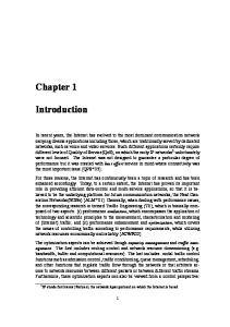
3.2 Encoding of Neural Networks To evolve an ANN, it needs to be expressed in proper form. There are some methods to encode an ANN like binary representation, tree, linked list, and matrix. Representation used here to encode an ANN is matrix encoding (Ahn and Cho, 2001). If N is the total node number of an ANN including input, hidden, and output nodes, the matrix is NxN, and its entries consist of connection links and corresponding weights. In the matrix, upper right triangle (Figure 7) has connection link information which describes 1 when there exists connection link and 0 when there is no connection 21
link. Lower left triangle describes the weight value corresponding connection link information. Figure 7 shows an example of encoding of an ANN which has one input node, two hidden nodes, and one output node. In the figure, I1 describes one input node, H1 and H2 describes hidden nodes, O1 describes the output node.
Figure 7: Encoding an ANN
Important thing to note here is that there isn’t any notion of hidden layers. Any hidden node can be connected to any other hidden node that has a higher index (only feed forward connections).
3.3 Ensemble Initialisation Each ANN in the ensemble is generated with random initial weights and fullconnection. Initial weights and biases were assigned randomly between [–1, 1] and [0, 1] respectively. 20 such ANNs were generated as initial population with 9 and 13 input nodes for breast cancer and heart disease datasets respectively. Hidden nodes were taken to be 5 and 6 respectively. In each case there was 1 output unit, which had a binary output.
3.4 Partial Training – Baldwin Effect Each ANN is trained partially (200 epochs) with training data, at each fitness evaluation of the evolutionary computation, to help the evolution search the optimal architecture of ANN and is tested with validation data to compute the fitness. Standard Backpropagation algorithm is used for training and transfer function for each hidden and output unit is Sigmoid Function. This local search, applied at each evolution step, decreases the time needed to find an acceptable solution or in other words it reduces the number of generations required. It can be viewed as lifetime learning of an individual in the evolutionary process. This is called the “Baldwin effect”, named after the person who first observed this in biology (Baldwin, 1896). He first recognized the impact of adaptive behaviour of individuals on evolution and showed that ‘Lamarckism’ was not necessary to explain the learned behaviour that seems to propagate through the genes of successive generations, but that instead, the inherited character was the ability to learn, with a 22
profitable effect on the fitness of the individual. The same effect is used here in evolutionary algorithm applied to neural networks.
3.5 Fitness Evaluation and Speciation The fitness of ANN is recognition rate of validation data and computed using speciation technique. Raw fitness of an individual p, fraw,p, is the inverse of Mean Square Error (MSE) calculated per pattern, per output unit. Hence raw fitness:
fraw,p = 1 / MSEp
(3.1)
For the purpose of speciation fitness sharing technique (Goldberg, 1989) is used here. Fitness sharing decreases the increment of fitness of densely populated ANN space and shares the fitness with other space. Therefore, it helps genetic algorithm search various space and generate more diverse ANNs.
3.5.1 Sharing at Phenotypic Level Fitness sharing is done at the phenotypic rather than at genotypic level, i.e. distance between two individual is judged on the basis of their behaviour (phenotype), not on the basis of their architecture or weights (genotype). This is required because there isn’t one to one mapping between the genotypic distance and the phenotypic distance between two individuals. E.g. two ANNs can have very similar matrix encoding (as discussed in section 3.2) but at the time behave quite differently for a given (say) classification task.
3.5.2 Kullback-Leibler Entropy –As Distance Measure To measure the distance between two individuals on the basis of their behaviour we will use the output values produced by these individuals for the validation set data points. The modified Kullback-Leibler entropy is used to measure the difference of two ANNs. As discussed by Ahn and Cho (2001), the outputs of ANNs are not just likelihood or binary logical values near zero or one. Instead, they are estimates of Bayesian a posteriori probabilities of a classifier. Using this property, the difference between two ANNs is measured with modified Kullback-Leilbler entropy (Kullback and Leibler, 1951), which is called relative entropy or cross-entropy. This is a measure of the distance between two distributions p and q, and is defined as:
D ( p, q ) =
m
∑p i =1
i
log
pi qi
(3.2)
However, the entropy is not a true distance due to the fact that is not symmetric, i.e., D(p, q) ≠ D(q, p). To remedy this problem, we can define symmetric relative entropy as follows: D ( p, q ) =
p q 1 m pi log i + qi log i ∑ qi pi 2 i=1
23
(3.3)
Let p and q be output probability distributions of two ANNs which consist of m output nodes and are trained with n data. Then, the similarity of the two ANNs can be calculated by
D ( p, q ) =
qij pij 1 m n + qi log pij log ∑∑ 2 i =1 j = 1 pij qij
(3.4)
where pij means the ith output value of the ANN with respect to the jth training data. Two ANNs are more similar as the symmetric relative entropy gets smaller. This is used as the distance measure between two ANNs p and q.
3.5.3 Speciation by Fitness Sharing Using the distance measure discussed in section 3.5.3 the sharing function sh(dpq) is computed as follows:
d pq 1 − sh(d pq ) = σs 0
for 0 ≤ d pq < σ s
(3.5)
for d pq ≥ σ s
Here, σs describes the sharing radius which is an empirical parameter. Different values (0.5, 1, 2) for σs were tried, but most of the experimentation was done with σs = 1, which was found to be the best one among the three values. If the difference of the individuals is larger than σs, they do not share the fitness. Only the individuals which have smaller difference among them than σs can share the fitness. Finally the shared fitness of an individual p, fshared, p is calculated as:
f shared , p =
f raw, p
(3.6)
pop size
∑ Sh(d q =1
pq
)
3.6 Evolutionary Process In the evolution of Neural Networks, at a particular generation, the whole old population is replaced with the new one. This is known as a generational GA. Elitism is also used with generational GA. Elitism performs two actions: 1. It makes a copy of the individual with best raw fitness in the old pool and places it in the new pool, thus ensuring the most fit chromosome survives. 2. Similarly one individual with the best shared fitness is copied to the new pool. The whole evolutionary process, which involves roulette wheel selection, crossover and mutation, is described in the following subsections.
24
3.6.1 Roulette Wheel Selection To create the mating pool, on which the genetic operators will be applied, roulette wheel selection is used. Members of the mating pool are selected according to their shared fitness. The better the chromosomes are, the more copies they get in the mating pool. The selection process can be described as: 1. [Sum] Calculate sum of all chromosome fitnesses in population - sum S. 2. [Select] Generate random number from interval (0,S) - r. 3. [Loop] Go through the population and sum fitnesses from 0 - sum s. When the sum s is greater then r, stop and return the chromosome where you are. Above procedure will give us a new member for the mating pool. Steps 2 and 3 are to be carried out N times to find N members.
3.6.2 Crossover The crossover operator exchanges the architecture of two ANNs in the population to search ANNs with various architectures. The crossover operator here searches for similar sub-graphs in the two parents and swaps the two smaller sub-graphs to create two children (see figure 9)
Figure 8: Example of Crossover operator
In the population of ANNs, crossover operator selects two distinct ANNs randomly and chooses one hidden node from each selected ANN. These two nodes should be in the same entry of each ANN matrix encoding of the ANN to exchange the architectures. Once the nodes are selected, the two ANNs exchange the connection links and corresponding weights information of the nodes and the hidden nodes after that. Figure 8 shows 25
an example of crossover. In this example, two ANNs have one input node, three hidden nodes, and one output node. When the H2 node is selected as crossover points, they exchange connection links and weights information of the selected entries.
Figure 9: Crossover - exchanging sub graphs
3.6.3 Mutation The mutation operator changes a connection link and a corresponding weight of a randomly selected ANN from the population. Mutation operator performs one of the two operations, which are: 1.
Connection Creation Mutation operator selects an ANN from the population of ANNs randomly and chooses one connection link from it. If the connection link does not exist and the connection entry of the ANN matrix is 0, the connection link is added. It adds new connection link to the ANN with random weights.
26
2.
Connection Deletion If the connection link already exists, the connection is deleted. It deletes the connection link and weight information.
Figure 10: Example of Mutation operator
Figure 10 shows two examples of the mutation. Upper one presents an example of connection creation. Since the selected connection link between I1 and H3 does not exist, the mutation operator adds a new connection link with weight 0.2 which is randomly generated between 0.0 and 1.0. The other one presents an example of connection deletion. The selected connection link between I1 and H3 with weight 0.2 has been deleted from the node after mutation.
3.7 Full Training The ANNs after the last generation are trained fully. After fixed number of generations, ANNs in the population are trained for 1000 epochs to fine-tune the weights.
3.8 Combining the Outputs The final result is obtained by combining the results of the individuals in the fully trained population. Output of each ANN is combined using the following three linear combination methods:
3.8.1 Majority Voting Here the output of the most number of ANNs will be the combined output. In case of a tie, the output of the ANN (among those in the tie) with the lowest error rate on the validation set is selected as combined output.
27
3.8.2 Averaging In this method the combined output is the average of the outputs of all individuals present in the final population.
3.8.3 Recursive least square (RLS) This method was used by Yao and Liu (1998a) to find the ensemble output of their EANNs. In this method weights are assigned to different ANN in the population and weighted average was calculated for the population. These weights are obtained by recursively updating the mean square error and minimising it. The mean square error based on training and validation set is N E = ∑ d (i ) − ∑ w j o j (i ) i =1 j =1 M
2
(3.7)
where M is the number of training plus validation examples and d(i) is the desired output for example i. Error given in (3.7) is for one output unit per ANN, which is the case for both the problems (only one output unit is required for binary classification). Minimising the error E with respect to weight wk yields M N ∂E = − 2∑ d (i ) − ∑ w j o j (i ) ok (i ) = 0 ∂wk i =1 j =1
(3.8)
Equation (3.8) can be expressed in matrix form roo w = rod
(3 . 9 )
where M
roo = ∑ o(i )o T (i )
(3.10)
i =1
and M
rod = ∑ d (i )o(i )
(3.11)
i =1
A unique solution to (3.9) exists if the correlation matrix roo is nonsingular. The weight vector w could be found by inverting roo and multiplying it by rod according to (3.9). However, this method is timeconsuming because whenever a new training example becomes available it requires inversion and multiplication of matrices. The RLS algorithm (Mulgrew and Cowan, 1988) uses a different method to determine the weights. From (3.10) and (3.11) we can get
roo (i ) = roo (i − 1) + o(i )o T (i ) And
28
(3.12)
rod (i ) = rod (i − 1) + d (i )o T (i )
(3.13)
Using (3.9), (3.12) and (3.13)
w (i ) = w (i − 1) + k (i )e(i )
(3.14)
Where
e(i ) = d (i ) − w T (i − 1)o(i )
(3.15)
And
k (i ) = roo−1 (i )o(i )
(3.16)
A recursion for r00-1 (i) is given by (3.7.8)
roo−1 (i ) = roo−1 (i − 1) −
roo−1 (i − 1)o(i )o T (i )roo−1 (i − 1) 1 + o T (i )roo−1 (i − 1)o(i )
(3.17)
In the implementation of the above RLS algorithm, three runs were always performed with different initial r00-1(0) and weights w(0). The initial weights were generated at random in [0, 0.1]
roo−1 (0) = αI N
(3.18)
where α = 0.1, 0.2, and 0.3 and IN is an NxN unit matrix. The best result out of the three runs was chosen as the output from the RLS algorithm and was also used to find the output for the testing set.
29
Chapter 4 Experimentation and Intermediate Results Experiments were conducted for both the benchmark problems in two stages. Initially only training and testing sets were used to evolve ANNs. i.e. both training and fitness evaluation were done on same set. The results obtained with this setup were not satisfactory, though the error rate for training data was acceptable but the error rate for testing data was much bigger than the already known results for the benchmark problems. To improve this generalisation error, need for the use of validation set was felt. So another set of experiments were conducted in which for the fitness evaluation of ANNs, a separate data set was used. The total data set for each benchmark problem was divided into 3 parts – Training, validation and testing set (As discussed in section 3.1). This section gives some of the intermediate results (regarding training and evolution of ANNs) and the final results for stage 1 of experimentation. Various parameters used in these experiments are given in table 1. Stage 1: Experiments Without Validation Set Parameter # of input nodes Maximum # of hidden nodes # of output nodes Population size Learning rate for training Data points in training set Data points in testing set SEED Crossover probability Mutation Probability Sharing Radius1 # of Generations # of Runs
Breast Cancer Dataset 9 5 1 20 0.1 350 349 System time 0.3 0.1 1 200 17
Heart Disease Dataset 13 6 1 20 0.1 200 70 System time 0.3 0.1 1 350 32
Table 1: Parameter Settings for Stage 1 Experiments
There were two important points observed from these experiments –
1
Initially three values were tried, 0.5, 1 and 2. Sharing radius = 1 repeatedly gave better results.
30
•
First one of course is that the generalization ability of these evolved ANNs was poor.
•
The second observation was the relative difficulty of classification of the two datasets – even for training, breast cancer dataset was much easier to classify than the heart disease dataset. The latter one required 350 generation of GA to achieve an acceptable error rate as compared to only 200 generations required in the former one. The results given in tables 2,3,4 and 5 further confirm this observation.
The number of runs for the heart disease dataset was not sufficient for any conclusive results but no further experimentation was conducted because of the poor generalisation ability of the evolved networks. Following subsections give some of intermediate results as examples of the training and evolution of ANNs. All results in subsection 4.1 and 4.2 are from a simulation run on the breast cancer dataset. Section 4.3 gives completes results for first stage of experimentation. And finally section 4.4 gives the parameter settings for the stage 2 of experimentation; final results for stage 2 experiments are given in section 5.
4.1 Training Results Figure 11 shows the partial training of the 20 individuals in the 0th generation. Figure 12 shows the full training of 20 individuals after 349th generation. Though it appears that the on an average error rate has increased from 0th to the 349th generation, in fact the average SSE after the training at 0th and after 349th generation is almost equal. Here, instead of looking at the SSE we should look at shared fitness of the individuals in the population because our GA is trying to maximise the shared fitness. On an average shared fitness of the individuals is increasing (figure 13). 80
70
60
Partial training at 0th generation Breast Cancer Dataset (For All 20 Individuals in the Population)
SSE
50
40
30
20
10
0 1
21
41
61
81
101
121
141
161
181
# of Epochs
Figure 11: Partial Training at 0th Generation in a Simulation Run for Breast Cancer Problem
31
70 F u ll T rai n i n g after 350 g enerati on s B reas t Can cer Datas et ( F or A ll 20 I n di v i du als i n the Popu lati on )
60 50
SSE
40 30 20 10 0 1
101
201
301
401
501
601
701
801
901
# of epochs
Figure 12: Full Training after 349th Generation in a Simulation run of Breast Cancer Problem
4.2 Evolution Results Figure 13 shows the average shared fitness of the population, for every generation and also the fitness (shared) of the individual with the best shared fitness, present in the population. Since the average shared fitness is improving (figure 13), the combined classification accuracy of the individuals in the population should also improve. As an example if we take voting as our combination method for ANN outputs and plot the number of wrong classifications of the training data versus the number of generations, Figure 14 is what we get. As expected, with the number of generations, the number of wrong classifications is going down. 25 Shared Fitness Vs Number of Generations (Breast Cancer Problem)
Average Shared Fitnes s Bes t Shared Individual
Shared Fitness
20
15
10
5
0 1
51
101
151
201
251
301
# of Gen erati on s
Figure 13: Shared fitness Vs # of generations for breast cancer problem
32
90 80 # of wrong Classifications Using Voting (Breast Cancer Problem)
70 60 50 40 30 20 10 0 1
21
41
61
81 101 121 141 161 181 201 221 241 261 281 301 321 341 # o f Ge ne ratio ns
Figure 14: # of wrong classifications by the ensemble for the Breast Cancer Problem (using Voting)
4.3 Full Results for First Stage Experiments Following are the final results of stage 1 of experimentation for the two datasets.
4.3.1 Heart Disease Problem Table 2 and 3 list the training and testing error rates, respectively of the group of evolved ANNs, for the Heart Disease problem. These results are averaged over 32 runs. Mean, SD, Min, and Max indicate the Mean Value, Standard Deviation, Minimum and Maximum values respectively. Results are given for all three combination methods used – Voting, RLS and Averaging. Voting Mean SD Min Max
0.1875 0.032 0.135 0.275
α = 0.1 0.1825 0.0273 0.115 0.265
RLS α = 0.2 0.1746 0.0261 0.125 0.26
α = 0.3 0.165 0.0245 0.105 0.25
Averaging 0.1975 0.0291 0.135 0.27
Table 2: Training Error Rates (stage 1) for Heart Disease Problem Voting Mean SD Min Max
0.3554 0.0424 0.2714 0.4143
RLS α = 0.3 0.2971 0.0296 0.2429 0.3714
Averaging 0.3472 0.0394 0.2571 0.4
Table 3: Testing Error Rates (stage 1) for Heart Disease Problem
33
4.3.2 Breast Cancer Problem Table 4 and 5 list the training and testing accuracies, respectively of the group of evolved ANNs, for the Breast Cancer problem. These results are averaged over 17 runs. Mean, SD, Min, and Max indicate the Mean Value, Standard Deviation, Minimum and Maximum values respectively. Results are given for all three combination methods used – Voting, RLS and Averaging. Voting Mean SD Min Max
0.0349 0.0275 0.0171 0.0457
α = 0.1 0.0266 0.0286 0.0143 0.04
RLS α = 0.2 0.0271 0.0295 0.0143 0.0343
α = 0.3 0.0198 0.0245 0.0114 0.0314
Averaging 0.039 0.0239 0.0171 0.0486
Table 4: Training Error Rates (stage 1) for Breast Cancer Problem Voting Mean SD Min Max
0.3092 0.0334 0.2378 0.3582
RLS α = 0.3 0.211 0.0276 0.1719 0.2779
Averaging 0.2964 0.0304 0.2292 0.3582
Table 5: Testing Error Rates (stage 1) for Breast Cancer Problem
If we compare the achieved error rates with some of the available results in literature (for heart disease problem – Yao and Liu (1998) and for breast cancer problem – Ahn and Cho (2001)), we will find that the though training error rates are close to the available results, but the testing error rates are too big and far from acceptable. Stage 2: Experiments With Validation Set Parameter # of input nodes Maximum # of hidden nodes # of output nodes Population size Learning rate for training Data points in training set Data points in validation set Data points in testing set SEED Crossover probability Mutation Probability Sharing Radius2 # of Generations # of Runs
Breast Cancer Dataset 9 5 1 20 0.1 349 175 175 System time 0.3 0.1 1 200 30
Heart Disease Dataset 13 6 1 20 0.1 135 67 68 System time 0.3 0.1 1 350 24
Table 6: Parameter Settings for Stage 2 Experiments
2
Initially three values were tried, 0.5, 1 and 2. Sharing radius = 1 repeatedly gave better results.
34
To improve this generalization another set of experiments were conducted including the validation set. The only difference between the two set of experiments besides the use of validation set is the way the ANNs are initialised. In the first stage of experimentation ANNs weren’t fully connected at the beginning but in the second stage they were. As we will see that there was as improvement in the results achieved but individual effects of the two modifications still needs to be studied. The final results obtained and their comparison with available results is given in section 5.
4.4 Parameter Settings for Stage 2 Experiments Table 6 lists the parameters for the next stage of experiments these parameters are identical with the previous ones except for the number of runs and the number of data points in training, testing and validation sets.
35
Chapter 5 Results and Discussion Table 7 lists the training, validation and testing error rates obtained by the group of evolved ANNs, for the breast cancer problem. These results are averaged over 30 runs.
Voting Training Validation Testing Mean 0.0378 0.0189 0.0231 SD 0.0100 0.0153 0.0176 Min 0.0074 0.0000 0.0000 Max 0.0544 0.0514 0.0514
Training 0.0374 0.0102 0.0078 0.0544
Averaging Validation 0.0235 0.0151 0.0114 0.0571
RLS Testing Training+Validation Testing 0.0229 0.0237 0.0167 0.0137 0.0152 0.0122 0.0000 0.0016 0.0000 0.0514 0.0267 0.0343
Table 7: Final Error Rates (averaged over 30 runs) for Breast Cancer Problem
Mean, SD, Min, and Max indicate the Mean Value, Standard Deviation, Minimum and Maximum values respectively. Results are given for all three combination methods used – Voting, RLS and Averaging. For RLS training and validation sets both were used to find optimal weights for the linear combination of outputs of neural networks, hence combined error for both training and validation sets is given. Training error rates achieved are comparable to stage 1 experiments but there is a significant improvement in the generalisation ability of evolved group of ANNs. There were runs in which zero wrong classifications were obtained in the testing set. The best results were obtained using RLS method for combining the outputs on an average. Though RLS always produced best results on training data but there were runs in which voting or averaging method produced better results in terms of testing errors. Table 8 lists the training, validation and testing error rates obtained by the group of evolved ANNs, for the heart disease problem. These results are averaged over 24 runs. More runs couldn’t be done because of shortage of time, as we will in section 5.3 running the algorithm is expensive. Again significant improvement in generalisation is achieved from stage one experiments. Even training error rates obtained here are lower than stage 1 experiments. This can only be attributed to change in the way the networks were initialised in the two stages. Otherwise we should expect the same errors.
36
Mean SD Min Max
Voting Averaging Training Validation Testing Training Validation 0.1960 0.1623 0.1642 0.1733 0.1828 0.0282 0.0265 0.0404 0.0231 0.0293 0.1333 0.1194 0.1176 0.1333 0.1194 0.2667 0.2388 0.2794 0.2370 0.2388
RLS Testing Training+Validation 0.1612 0.1462 0.0323 0.0243 0.1029 0.1188 0.2353 0.2129
Testing 0.1612 0.0337 0.1176 0.2500
Table 8: Final Error Rates (averaged over 24 runs) for Heart Disease Problem
In general we have achieved lesser error rates on validation sets than on training set, this is because our GA is trying to maximise the fitness which was calculated over the validation set. One thing worth mentioning here is the relative degree of difficulty of classification in the two datasets. In heart disease, even after 350 generations, error rates are pretty big in comparison to the heart disease dataset. So heart disease dataset proves to be much harder to classify.
5.1 Comparison with known results 5.1.1
Breast Cancer problem
Ahn and Cho (2001) obtained 1.71% test error rate as their best result using single linkage clustering and voting and averaging combination methods. The best result here was achieved by using RLS. On an average over 30 runs RLS combination method produced 1.67% error rate on test set, which is better than Ahn and Cho’s result. But voting and averaging methods produced 2.31 and 2.29% error rates respectively, which are higher.
5.1.2
Heart Disease problem
Yao and Liu (1998) obtained 5.8% and 15.1% error rates, for training and testing datasets, as their best results for the heart disease problem. The best results achieved here are 14.62% and 16.12% respectively for the two sets. Though the testing error rate is comparable the training error rate is much higher.
5.2 Comparing best individual performance with combination methods Just to see how useful these combination methods are in comparison to the best individual present in the population, their performance (on training set3) is plotted with the performance of best individual present in the population for the two problems. Figures 15 and 16 give error rates versus the number of generations for the best individual and for all 3 combination methods used here.
5.2.1 Breast Cancer problem
3
For RLS both training and validation sets are used
37
For the Breast cancer problem (figure 15) the combination methods except the RLS prove to be worse than the best individual present in the population. Few observations can be made from this plot:
•
It took around 125 generations for voting and averaging to reach the performance comparable to RLS or of the best individual. One possible reason for the bad performance of voting and averaging can be – their performance is measured on training set while the fitness evaluation is done on the validation set. On the other hand error rates for the RLS method is based on both training and validation sets.
0.25
Error Rates on Training Set f or Breas t Cancer problem ( Comparing Combination methods with Best Individual bes t indiv idual in the population) Voting
0.2
Error Rates
Averaging 0.15
RLS
0.1
0.05
199
190
181
172
163
154
145
136
127
118
109
100
91
82
73
64
55
46
37
28
19
10
1
0
# of generations
Figure 15: Error Rates for the best individual and combination methods for Breast Cancer Problem
•
The best individual is almost as good as the best combination method (RLS). So the classification problem being easy – these methods aren’t exploited to their full extent. We will see (section 5.2.2) that for a much harder problem these methods turn out to be useful and perform much better than the best individual.
5.2.2 Heart Disease Problem For the Heart Disease problem (figure 16), it turns out that the combination methods perform much better than the best individual present in the population. Few observations can be made from this plot:
•
RLS again gives the best performance, though averaging also performs quite well. Voting on the other hand performs no better than the best individual.
•
In this problem the difference between – using the best individual and using the full population is visible.
•
This difference becomes more prominent when we look at the performance on test set. For the same run (for which the plot has been provided) the best 38
individual produced 17 wrong classifications out of 68 patterns in test set, i.e. 25% error rate while voting, averaging and RLS produced – 17.65%, 19.12 and 17.65% error rates.
0.49 0.44
Error Rates f or H eart Dis eas e Problem ( Comparing Combination Methods with the Bes t Indiv idual in the Population)
Error Rates
0.39 0.34
Best Individual Voting Averaging RLS
0.29 0.24 0.19 0.14 0.09 1
21
41
61
81
101 121 141 161 181 201 221 241 261 281 301 321 341
# of Generations
Figure 16: Error rates for the best individual and various combination methods for Heart Disease problem
5.3 Complexity of Algorithm One run of the programme took 3 hours for heart disease problem (350 generations) and 2 hours 30 minutes for breast cancer problem (200 generations) to run. Lets look at the time complexity of the algorithm in this section. The algorithm consists of partial training at each evolution step and the standard fitness sharing. Combination of outputs was carried out using a separate code. Here we will look at the algorithm that evolves the ANNs. Training of an ANN consists of two major phases, the first of which is the feed forward of the training input. Essentially, this phase consists of multiplying each input vector element by the weight residing on its connection to a node in the hidden layer. Then, a sum is taken over all connections to that hidden layer node to obtain the hidden unit's net input. This process is then repeated for passage of the signal from the hidden layer to the output layer. Now, if there are 'n' input units, 'm' hidden units, and 'k' output units, the dot products will require
m(n+logn) + k(m+logm) operations. And neglecting logn with respect to n, we get O(nm+km) as a lower bound for the time complexity of the feedforward phase. Roughly speaking training
39
algorithm as whole will take just the double time of feed forward phase. So, even for full training phase we get O(nm+km) as the lower bound for time complexity. In every generation this has to be done N number of times, where N is the population size. And this process will continue the given number of generations, say G. Standard fitness sharing requires O(N2) computations, where N is the population size. So an estimate of lower bound of time complexity of full algorithm can be:
O((m(n+k) * N + N2) * G) For the two benchmark problems taken these parameters used were: • Breast Cancer – m=5, n=9, k=1, G=200, N=20 • Heart Disease – m=6, n=13, k=1, G=350, N=20 So the least number of computations for the two problems become 280,000 and 728,000 for the two problems respectively. Hence for a 500 MHz machine it will take at least 9.3 min and 24. 27 minutes to run.
40
Chapter 6 Conclusion In the first part of the project various niching and speciation techniques were explored. It was observed that standard niching technique (fitness sharing) was unable to deal with problems having irregular unevenly spaced peaks in multi-dimensional spaces. Besides that, due to distance calculations it was also found to be expensive. It also required the prior knowledge of fitness landscape for optimal parameter settings. Sharing tries to distribute the individuals over a larger area and hence instead of having many individuals very close to the peaks, it tends to spread the individuals around the peaks. Using niching and speciation both can solve the last problem, but still the process will be expensive and furthermore, information about the fitness landscape will still be needed. Some of the recent niching and speciation techniques were explored in order to find solutions to some of these problems. Adaptive Clustering (section 2.3.1) and collective sharing (section 2.3.3) reduced some amount of priory knowledge about the fitness landscape but they two required information about maximum and minimum size of clusters. Out of the various schemes explored DNC (section 2.3.4) required the least amount of prior knowledge about the fitness landscape, it only requires the knowledge of the dimensionality and the bounds of the search space. Another modification of DNC with fuzzy radius niching (section 2.3.6) was proposed by the same authors, to make it efficient, in which Hill-valley fitness topology function was used for the local analysis of fitness landscape. The same function was also used by multi-national EA (section 2.3.5) to explore the search space better and to adapt its search strategy to the problem. The second part of the project involved implementation of a system that evolves a group of neural networks using GA with simple fitness sharing. Sharing was performed at phenotypic level using modified Kullback-Leibler entropy as the distance measure. To make use of population information present in the final generation of GA, the final result was obtained by combining the output of all the individuals present in the final population using various linear combination techniques – voting, averaging and RLS. The developed system was tested on two benchmark datasets from UCI benchmark datasets, namely Wisconsin Breast Cancer Dataset and Heart Disease Dataset. It was observed that the breast cancer dataset was much easier to classify than the heart disease dataset.
41
Significantly better results were achieved by using a validation set. Out of the three combination methods RLS produced the best results. Combination of outputs produced much better results than the best individual in the harder problem (heart disease problem). Results achieved for Breast Cancer problem were better than known results available. Comparable results were also achieved in Heart Disease problem. Though the evolved system performed quite well on the two benchmark problem taken, still there are some criticisms too. First one obviously is that it is too expensive and should not be applied to relatively easier problems like the breast cancer problem, where it cannot be exploited to its full extent. Another drawback of the system is the choice of sharing radius, which was chosen empirically. In the earlier stages of experimentation only three values were tried and the best one was chosen for the rest of experiments. More experimentation couldn’t be done as running the code was quite expensive. More experiments with different values of sharing radius could have produced better results. As discussed in section 2.1.1, the requirement of priori knowledge about the fitness landscape (in our case the sharing radius) was one of the limitations of standard fitness sharing technique. Thus an obvious modification to the system can be – the use of one of the niching or speciation techniques discussed in section 2.3. Some of the future work directions, including this one, have been discussed in the following sub-section.
6.1 A different speciation technique Multi-national EA and DNC with fuzzy variable niching were the two most promising techniques discussed in section 2.3. A possible extension of this project is to implement one of these in the EANN system. Both of these schemes use hill-valley fitness topology function which allows the local analysis of the fitness landscape and thus help them in making more informed decisions, based on this analysis, about merging and splitting or merging and migrating two species in the two schemes respectively. Implementing DNC will not only help in terms of reducing the running time (as the complexity of DNC is O(pq) as compared to O(p2) in standard fitness sharing ) but it will also eliminate the requirement of setting a value for niching radius.
Figure 17: Black box crossover operator
42
6.2 A different Crossover Operator The crossover operator used here (section 3.6.2) exchanges the similar sub graphs in the two parents. But as the ANNs here aren’t very complicated many times it happens that the sub graph chosen turns out to be the full network – hence parent 1 becomes child 2 and parent 2 becomes child 1. Thus many times it doesn’t do anything and just changes the two parents. Another possible crossover operator could be (say) A Black Box Crossover Operator (figure 17). This will search for black boxes (which can contain any number of units) having same number of connections coming out. Starting from one single node randomly – it will search for bigger black boxes and once such boxes are found in the two networks it will swap them to produce two offspring.
6.3 Another Combination Method – Weighted Voting A voting arrangement in which voters may control unequal number of votes and decisions are made by forming coalitions with the total of votes equal or in access of an agreed upon quota is called a weighted voting system. This combination method can be used to improve the generalization ability of the ensemble. Main idea behind this method is to provide more voting power to those ANNs which perform better on training data points which are similar to the given testing data point. For every given testing data, distance (Euclidian) with every data point will be calculated and the closest one will be chosen. Now weights will be assigned to different ANNs depending upon whether it classified this chosen training data point correctly or not.
6.4 Choosing representative of each species in the final population Ahn and Cho (2001) used single linkage clustering method to choose the representatives of each species present in the final generation. Outputs of only these representatives were combined to obtain the final output. They achieved better results by using these representatives instead of the full population. This variation can also be tried.
43
References [1]
Ahn, J. H. & Cho, S. B., 2001, Speciated Neural Networks Evolved with Fitness Sharing Technique. Proceedings of the 2001 Congress on Evolutionary Computation, 390-396, Seoul, Korea.
[2]
Baldwin, J. M., 1896, A New Factor in Evolution. American Naturalist, 30, 441–451.
[3]
Cover, T., & Thomas, J., 1991, Elements of Information Theory, Wiley Series in Communications, New York.
[4]
Darwen, P., & Yao, X., 1996, Automatic Modularization by Speciation.
Proceedings of the 1996 IEEE International Conference on Evolutionary Computation (ICEC '96), 88-93, Nagoya, Japan: IEEE Computer Society Press. [5]
Deb, K. & Goldberg, D., E., 1989, An Investigation of Niche and Species Formation in Genetic Function Optimisation. Proceedings of the Second International Conference on Genetic Algorithms (ICGA), 42-50, Hillsdale.
[6]
De Jong, K. A., 1975, An Analysis of the Behaviour of a Class of Genetic Adaptive Systems. Doctorial Dissertation, University of Michigan. Also Dissertation Abastract Int.5140B (University Microfilms 76-9381).
[7]
Gan, J. & Warwick, K, 1999, A Genetic Algorithm with Dynamic Niche Clustering for Multimodal Function Optimisation. In proc. of the 4th Inter. Conf. on Artificial Neural Networks and Genetic Algorithms, 248-255, Springer Wien New York.
[8]
Goldberg, D. & Richardson, J, 1987, Genetic Algorithms with Sharing for Multimodal Function Optimization. Proceedings of the 2nd Inter. Conf. on Genetic Algorithms, 41-49.
[9]
Goldberg, D., 1989, Genetic Algorithms in Search, Optimization and Machine Learning, Addison-Wesley, Reading Massachusetts.
[10]
Kullback, S., & Leibler, R. A., 1951, On Information and Sufficiency. Ann.
Math. Stat., 22, 79~86. [11]
Mahfoud, S. W., 1992, Crowding and Preselection Revisited. Parallel Problem Solving From Nature, 2, Manner, R., & Manderick, B.(eds), 27-36, Elsevier Science Publishers, Amsterdam.
[12]
Mahfoud, S. W., 1995, Niching Methods for Genetic Algorithms. Doctoral dissertation, University of Illinois at Urbana-Champaign, Urbana. Also IlliGAL Report No. 95001.
[13]
Mulgrew, B. & Cowan, C. F. N., 1988, Adaptive Filters and Equalizers. Boston, MA, Kluwer.
44
[14]
Pictet, O. V., Dacarogna, M. M., Davé, R. D., Chopard, B., Schirru, R. & Tomassini, M, 1995, Genetic Algorithms with Collective Sharing for Robust Optimization.Financial Applications, Olsen & Associates Working Paper (OVP.1995-02-06).
[15]
Spears, W. M., 1994, Simple Subpopulation Schemes. Proceedings of 3rd Annual conf. on Evolutionary Programming, 296-307, World Scientific.
[16]
Ursem, R., 1999, Multinational Evolutionary Algorithms. Proceedings of
Congress of Evolutionary Computation, 3, 1633-1640. [17]
Yao, X. & Liu, Y., 1998a, A New Evolutionary System for Evolving Artificial Neural Networks, IEEE Trans. Neural Networks, 8, 694-713, Anchorage, USA.
[18]
Yao, X. & Liu, Y., 1998b, Making Use of Population Information in Evolutionary Artificial Neural Networks. IEEE Transactions on Systems, Man and Cybernetics, Part B: Cybernetics, 28(3), 417-425.
[19]
Yao, X., 1999, Evolving Artificical Neural Networks, Proceedings of the
IEEE, 87(9), 1423-1447. [20]
Yin, X. & Germay, N, 1993, A Fast Genetic Algorithm with Sharing Scheme Using Cluster Analysis Methods in Multimodal Function Optimization. Proc. Inter. Conf. Artificial Neural Nets and Genetic Algorithms, 450- 457, Innsbruck, Austria.
The references have been prepared using:
Bibliography Styles Handbook, American Psychological Association, Publication Manual (4th ed). [Available online at] http://www.english.uiuc.edu/cws/wworkshop/bibliography/apa/apamenu.htm
45
Appendices Appendix A: Mini-project declaration Appendix B: Statement of information search strategy Appendix C: Benchmark Problems
46
Appendix B: Statement of information search strategy Parameters of literature search Most of the literature search was carried out for the first part of the project in which search for various niching and speciation techniques were searched for.
Forms of literature The category explored maximally was conference papers; Journal articles, theses books and www pages were also searched for.
Age-Range of literature D. E. Goldberg and J. Richardson first introduced fitness sharing in 1987. So the search was carried out from 1987 onwards.
Restrictions as to language I don’t know any other language than English so my search will be limited to articles published in English only.
Appropriate search tools Engineering Index Ei Compendex (http://edina.ac.uk/compendex/login.shtml), can be used to search interdisciplinary engineering information database in the world. Various keywords can be used to search for conference papers, journal articles and some theses.
Science Citation Index (SCI) This was used for finding relevant journal papers. Cited reference search was also performed using SCI. In SCI keywords can be used to find some papers to start with, further cited reference search can be used. ResearchIndex (http://citeseer.nj.nec.com/cs) and Web of Science (http://wos.mimas.ac.uk) are two useful science citation indices.
Dissertations Abstracts International (DAI) and Index to Theses DAI (http://wwwlib.umi.com/dissertations/gateway) can be used to retrieve North American theses and Index to Theses (http://www.theses.com) can be used to retrieve UK theses.
47
Search statements The search statements will be based on following terms: Evolving, Artificial, Neural, Networks, Speciation, Niching, Fitness Sharing, Crowding, Modularisation – various combinations of these keywords were used. E.g. 1. Evolving AND Artificial AND Neural AND Network 2. Speciation AND Niching OR Fitness AND Sharing 3. Automatic AND Modularisation etc.
Brief evaluation of the search For the first part of the project, using various keywords for searching in Science Citation Index, following 18 items were retrieved.
• 10 journal Articles • 15 Conference papers • 3 PhD Theses Using these as starting points, cited reference search was carried out. For the second part of the project, my project supervisor suggested one important paper. Other literature items were retrieved by the cited reference search. From the above two sources, finally following relevant items were chosen.
• • • •
5 Journal articles 9 conference papers 2 books 1 working paper
48
Appendix C: Benchmark Problems
Heart Disease Database 1.
Number of instances: 270
2.
Number of attributes: 13 (which have been extracted from a larger set of 75) plus the class attribute.
3.
Attribute Information: 1. age 2. sex 3. chest pain type (4 values) 4. resting blood pressure 5. serum cholestoral in mg/dl 6. fasting blood sugar > 120 mg/dl 7. resting electrocardiographic results (values 0,1,2) 8. maximum heart rate achieved 9. exercise induced angina 10. oldpeak = ST depression induced by exercise relative to rest 11. the slope of the peak exercise ST segment 12. number of major vessels (0-3) colored by flourosopy 13. thal: 3 = normal; 6 = fixed defect; 7 = reversable defect
4.
Attributes types 1. 2. 3. 4.
Real: 1,4,5,8,10,12 Ordered:11, Binary: 2,6,9 Nominal:7,3,13
5.
Variable to be predicted –Absence (1) or presence (2) of heart disease
6.
No missing values.
Wisconsin Breast Cancer Database 1.
Sources:
Dr. WIlliam H. Wolberg (physician) University of Wisconsin Hospitals Madison, Wisconsin USA Donor: Olvi Mangasarian (
[email protected]) Received by David W. Aha (
[email protected]) Date: 15 July 1992 2.
Number of Instances: 699
3.
Number of Attributes: 10 plus the class attribute
49
4.
Attribute Information: (class attribute has been moved to last column)
# Attribute Domain -- ----------------------------------------------------------------------1. Sample code number id number 2. Clump Thickness 1 - 10 3. Uniformity of Cell Size 1 - 10 4. Uniformity of Cell Shape 1 - 10 5. Marginal Adhesion 1 - 10 6. Single Epithelial Cell Size 1 - 10 7. Bare Nuclei 1 - 10 8. Bland Chromatin 1 - 10 9. Normal Nucleoli 1 - 10 10. Mitoses 1 - 10 11. Class: (2 for benign, 4 for malignant) 5.
Missing attribute values: 16
There are 16 instances in Groups 1 to 6 that contain a single missing (i.e., unavailable) attribute value, now denoted by "?". 6.
Class distribution: Benign: 458 (65.5%) Malignant: 241 (34.5%)
50