Chapter 1: Exercises - correction
1. Solving the job search model with explicit wage distributions In the various cases, the reservation wage x solves Z 1 w x x =b+m r+q x The hazard rate is
= m [1
(w) dw
(1)
(x )], and the post-unemployment wage is w =
R1 x
w1
(w) (x ) dw.
The
job o¤er rate m only a¤ects w through changes in the reservation wage x . As dx =dm > 0, dw=dm > 0. The marginal impact of m on
results from d =dm = 1
(x )
m (x ) dx =dm
(2)
Overall impact is ambiguous. 1.1 For all b 2 [0; 1], I obtain
i r+q h 1=2 (1 + (1 b) 2m=(r + q)) 1 (3) m h i 1=2 x ) = (r + q) (1 + (1 b) 2m=(r + q)) 1 . It is increasing in m.
x =1 The hazard rate is
= m (1
1.2 I obtain
x The hazard rate is
= me
x
b=
= (r + q) (x
m e (r + q)
x
(4)
b). This trick shows that
is strictly increasing in m
(because x is strictly increasing in m).
x*
4
3
2
1
0 0.0
0.5
1.0
1.5
2.0
2.5
3.0
3.5
4.0
m
Reservation wage x as a function of the contact rate m - parameters are set to r = 5%,
= 1, b = 1=2.
This Figure can be obtained with any mathematical package –here Maple. 1.3 The equation to solve is the following: x =b+m
Z
1
x
w x exp r+q 1
h
2
(ln w) = 2 p w 2
2
i
dw
(5)
This cannot be solved analytically. Write T (x; m) = b + m writes
R1 x
2 =(2 w x exp[ (ln w) p r+q w 2
2
)]
dw. The model
x = T (x; m)
(6)
with T continuous, strictly decreasing, T (0) > b and T (1) = b < 1. These properties ensure that there
exists a unique x that you can …nd numerically. 1.4 Hazard rate is
= m [1
(wmin )]. Average unemployment duration is E (s) = 1= . So m no
longer a¤ects the min of the accepted wage distribution, and
is strictly increasing in m.
1.5 The reservation wage x now solves x =b
t+m
Z
1
x
w x r+q
(w) dw
(7)
and so dx =dt < 0. 2. Non-stationary search Anabella is unemployed. She does not receive unemployment bene…t and …nances her job search by dissaving. At time 0, her wealth is W0 . When her wealth reaches 0, she stops searching and stays unemployed forever. 2.1 Assuming that Anabella does not receive interest payments on her wealth during her job search, RT we have 0 cdt = W0 . Therefore, T = W0 =c. 2.2 Anabella’s expected utility writes rU (t)
= m [w=r
U (T )
= 0
U (t)] + U 0 (t)
( )
The explanation is given in the course. Note the terminal condition U (T ) = 0, which normalizes Anabella’s expected utility to 0 when she stops searching. The problem is stationary after t = T . Prior to T , the problem is nonstationary and we must solve the Cauchy problem ( ). This gives i mw h 1 e (r+m)(T t) rU (t) = r+m
(8)
You can check that U 0 (t) < 0. Utility decreases as the termination date becomes closer. The hazard rate is m (t) =
(
m if t
T
(9)
0 else
Wealth has a positive e¤ect on the hazard rate because it raises T . From this perspective, rich persons are less exposed to the risk of long-term unemployment as they can …nance their job search over longer periods. 2.3 Anabella’s expected utility now writes rU (t)
=
max
U (T )
=
0
e
:5e2 + me [w=r
U (t)] + U 0 (t)
( )
2.4 The …rst-order condition to problem ( ) is e (t) = m [w=r 2
U (t)]
(10)
We can replace this condition in problem ( ) to obtain the following Cauchy problem:
where P (x) = rx
:5m2 [w=r
U 0 (t)
= P (U (t))
U (T )
= 0
(11)
2
x] . You don’t need to solve it to get the main idea. The hazard rate is
me (t). As U 0 (t) < 0, the hazard rate increases over the duration of unemployment, until the termination date T . Duration-dependence here is non-monotonic: hazard is increasing at …rst, and then falls to 0. Note that equation (11) is a Riccati di¤erential equation, which admits explicit solutions. 2.5 Wealth impacts the hazard rate through its e¤ects on the termination date T . Writing U (t) = U (t; T ), one can notice that U (t; T ) = U (0; T
t). Changes in termination date are equivalent to
opposite changes in unemployment duration. It follows that e (t; T ) = e (0; T
t). Therefore eT =
et =
mUt (t; T ) < 0. Richer agents bene…t from a longer job search period. They are have less incentive to …nd jobs and the hazard rate is lower at all durations. However, the hazard rate is positive over a longer period. 3. Duration-dependent hazard rates 3.1 See course. 3.2 See course. 3.3 Be careful, in s = T high-hazard workers start searching for jobs and the hazard rate jumps upward. 3.4 Max problem is rU (s)
=
maxfb
rU
=
maxf c + m[wmin =r
U (s)] + U 0 (s); b + U 0 (s)g for s < T
c + m[wmin =r
U ]; 0g for s
T
(12) (13)
3.5 When c is too high, worker never searches. When c is 0, worker always searches. So there is [c0 ; c1 ] on which the worker starts searching at some date 2 (0; T ). So the problem becomes 8 0 > > < b + U (s) if s < rU (s) = b c + m[wmin =r U (s)] + U 0 (s) if s 2 [ ; T ) > > : c + m[w =r U (s)] if s > T min
(14)
with U ( ) = lims! U (s).
4. Frictions In the marriage market 4.1 Max problem is rU rW ( )
= m =
4.2 I obtain rU = m
Z
Z
maxfW ( )
U; 0g ( )d ;
+ q(U
W
1
rU qT ( )d : r+q
rU +qT
T ):
Let x = rU + qT be Annabella’s reservation beauty. I have Z 1 x x qT = m ( )d ; r + q x 3
(15) (16)
(17)
(18)
which shows that x increases with T . Marriage proba is reduced and mean attractiveness is increased. 4.3 We have rU
= m
Z
maxfM ( )
rM ( )
=
+ q(U
M( )
rN ( )
=
+ q(U
N ( )):
U; N ( )
U; 0g ( )d ;
T );
(19) (20) (21)
Whatever the value of being single U , we have M ( ) < N ( ). Annabella will never be married: commitment means potential cost T and there is nothing in return. For marriage to take place, marriage must have some value. For instance, marriage may reduce the separation rate q or increase the utility ‡ow derived from the relationship. 4.4 Marriage increases utility ‡ow: commitment creates speci…c investments, income tax may be reduced. 4.5 We have rU
Let S( ) = M ( ) qT =(A
= m
Z
maxfM ( )
rM ( )
= A + q(U
rN ( )
=
+ q(U
N ( ) = [(A
U; N ( )
M( )
U; 0g ( )d ;
T );
(23)
N ( )):
1)
(22)
(24)
qT ]=(r + q). So Annabella gets married whenever
>
1) > rU . She either stays single or enters a nonmarriage relationship otherwise.
5. Stochastic output and reservation wage 5.1 We have rW (y)
= w (y) + q [U W (y)] Z = b+m max fW (y)
rU
(25) U; 0g (y) dy
(26)
Y
Combining equations: rU = b + m
Z
max
Y
w (y) rU ;0 r
(y) dy
(27)
5.2 The reservation wage is such that w = rU . As w increases with y, the reservation wage is associated with the reservation output level w
1
(rU ). Therefore Z w (y) rU rU = b + m (y) dy r 1 y w (rU )
Consider the following change of variable ! = w (y). This leads to Z 1 ! x x=b+m (!) d! r+q x with
(!) =
w
1
(!) =w0 w
1
(28)
(29)
(!) .
Solving for a reservation productivity is equivalent to solving for a reservation wage. Then, we need to de…ne the wage distribution. This can be done from the output shock distribution. Indeed, Pr [w (y)
!] = Pr y
w 4
1
(!) =
w
1
(!)
(30)
5.3 The computation leads to x= One can check that x <
r+q m
1
1+2
m (1 r+q
b= )
1
(31)
. The lowest output level is x= . The hazard rate is 1
mean duration of unemployment is s =
= m [1
x], the
, and the mean post-unemployment wage is w = (1 + x) =2.
Parameter b has obvious e¤ects, while parameter
has ambiguous impacts.
5.4 We have rW (y) rU
Z
= y + q [U W (y)] + Z = b+m max fW (y)
Y
max fW (y 0 )
W (y) ; U
W (y)g (y 0 ) dy 0
U; 0g (y) dy
(32) (33)
Y
The reservation wage is such that W (x) = U . Similarly, once in the job, the worker stays employed whenever W (y 0 )
U . Therefore, he stays employed if and only if the wage is larger than the reservation
wage. Combining equations leads to (r + q + ) [W (y)
U] = y
rU +
Z
1
[W (y 0 )
U ] (y 0 ) dy 0
(34)
x
Integrating both sides of the equation leads to Z 1 Z [W (y) U ] (y) dy = x
1
x
It follows that rU = b + m
Z
1
x
Using the fact that W (x) = U , I obtain (m
y rU (y) dy r+q+ (x)
y rU (y) dy r+q+ (x)
) rU = mx
(35)
(36)
b
(37)
Combining the last two equations leads to x = b + (m
)
Z
1
x
The reservation wage is decreasing in
y x r+q+
(y) dy
(38)
. In the standard job-search model, the reason why a worker
rejects job o¤ers is because he knows that he won’t bene…t from another wage o¤er once in employment. He must be selective as a result. However, if output shocks lead to wage changes, he no longer needs to stay unemployed. For instance, x = b when m = . In this case, the worker accepts all wage o¤ers larger than unemployment bene…t b. 5.5 In steady state, unemployment in‡ows coincide with unemployment out‡ows: q (1
u) +
(x) = u [1
(x)]
(39)
This gives u. Similarly, ‡ows of workers in the group of employees paid at most w coincide with ‡ows out of this group. This gives q (1
u) F (w) + (1
u [ (w)
(x)] + (1
u) F (w) [1 u) [1
5
(w) +
F (w)] [ (w)
(x)] = (x)]
(40)
The solving gives F (w). The result for G (w) holds by construction. 6. Take-it-or-leave-it o¤ ers in the housing market 6.1 Let pS denote the seller price, while pB is the buyer price. Then, pS = y and pB = 0. Buyers’ and sellers’expected payo¤s are UB
=
y
US
=
(1
(41) )y
(42)
6.2 Let UB and US denote buyers’and sellers’expected utility. If a buyer makes an o¤er, he will o¤er the lowest price that the seller accepts. Therefore, pB = US . Symmetrically, pS = y rUB
=
(y
rUS
= (1
US
UB )
) (y
UB . It follows that (43)
US
UB )
(44)
y
(45)
y
(46)
The solving gives UB
=
US
=
The mean house price is p = pS + (1
r+
+ (1 (1 ) r+ + (1
) )
) pB . Therefore, p=
(1 ) r + (1 r+ + (1
) )
y
(47)
6.3 Seller’s o¤er is pS (y) = UB (y), while buyer’s o¤er is pB = US , with rUB (y)
=
rUS
=
[y (1
)
US Z
UB (y)] [y
(48)
UB (y)
US ] (y) dy
(49)
The solving gives UB (y)
=
US
=
Mean house price is p = US + (1
(1 r+
) y p = (1
(1
y
r+
r+
) + (1
)
) + (1
)
y
y
(50) (51)
UB (y) : )
r+ + (1
r+
6.4 Seller’s exepcted utility is US = max p
Z
1
)
y
p (y) dy
(52)
(53)
p
Increasing p has two e¤ects: rise in price if accepted, but decline inacceptance probability (if buyer’s willingness to pay is too low). First-order condition to the max problem gives p = [ (p)] 6
1
(54)
7. Reservation wage and sanctions against the unemployed 7.1 See course. 7.2 I obtain x The hazard rate is
= me
x
= r (x
b=
m e r
x
(55)
b). This trick shows that
is strictly increasing in m (because
x is strictly increasing in m).
x*
4
3
2
1
0 0.0
0.5
1.0
1.5
2.0
2.5
3.0
3.5
4.0
m
Reservation wage x as a function of the contact rate m - parameters are set to r = 5%,
= 1, b = 1=2.
7.3 We have for all b rU (b) = b + m
Z
Y
max fW (w)
U (b) ; p [U (0)
U (b)]g (w) dw
(56)
The novelty comes from the second term between brackets fg. In case the o¤er is rejected, the worker is sanctioned with proba p. In this case, he loses bene…ts.
7.4 The reservation wage is such that W (x (b)) = U (b) + p [U (0) x (b) = rU (b) + p [rU (0)
rU (b)]
U (b)]. This gives (57)
As x0 (b) has the sign U 0 (b) and U 0 (b) > 0, we have x (b) > x (0). Increasing p makes o¤er rejection more costly as workers lose bene…t entitlement with increased probability. The reservation wage, therefore, decreases with p. 7.5 Bene…t generosity b may be compensated by a higher sanction probability p. Therefore, xD < xF , D
>
F
and sD < sF .
8. Reconsidering the e¤ ects of unemployment insurance 8.1 The model assumes that searching for jobs has a psychological cost, for instance in terms of foregone leisure. Similarly, working has a psychological cost measured by the negative marginal impact of 7
e on the marginal utility v. The condition v (h; w) > v (0; b) means that an employed worker fare better than a non-employed individual who decides not to seek jobs. 8.2 The expected utility of an unemployed person writes rU = max fv (e; b) + me [W (w)
U ]g
e
(58)
8.3 The …rst-order condition to the maximization problem writes ve (e ; b) = m [v (h; w) =r
U]
(59)
8.4 Using the implicit function theorem, de = db 8.5 The sign of de =db depends on veb (e ; b)
U 0 (b) + veb (e ; b) vee (e ; b)
(60)
U 0 (b). Unemployment bene…ts have two e¤ects. On
the one hand, they raise the value of unemployment, which tends to deteriorate search investments. This is the moral hazard e¤ect of unemployment compensation emphasized during the course. On the other hand, unemployment bene…ts may a¤ect the marginal cost of search e¤ort through the cross derivative veb . When veb < 0, de =db < 0. This corresponds to gross complementarity between consumption and leisure. When veb > 0, de =db can be positive, so that search investments increase with unemployment bene…ts. This corresponds to gross substitutability between consumption and leisure. The degree of substitutability between consumption and leisure in individual preferences varies across individuals. So, unemployment bene…ts may boost search e¤orts among individuals who easily substitute a loss in leisure by an increase in consumption.
8