CALL TRANSCRIPT SEGMENTATION USING WORD COOCCURRENCE MODEL Shajith Ikbal
Karthik Visweswariah
IBM Research, Bangalore, India. {shajmoha, v-karthik}@in.ibm.com
ABSTRACT In this paper, we propose a word cooccurrence model to perform topic segmentation of call center conversational speech. This model is estimated from training data to discriminatively represent how likely various pairs of words are to cooccur within homogeneous topic segments. We show that such model provide an effective measure of lexical cohesion and hence provide useful evidence of topical coherence or lack thereof between various parts of the call transcripts. We propose two approaches of utilizing such evidence for segmentation: 1) An efficient dynamic programming algorithm to perform segmentation simply utilizing the word cooccurrence model. 2) Extracting features based on word cooccurrence model to utilize them as additional features in conditional random field (CRF) based segmentation. Experimental evaluation of these approaches against state-of-the-art approaches show the effectiveness of word cooccurrence model for the topic segmentation task. Index Terms— topic segmentation, word cooccurrence, dynamic programming algorithm, conditional random field, complementary features. 1. INTRODUCTION The aim of topic segmentation of audio conversations is to automatically estimate topically coherent homogeneous segments from the corresponding transcripts [1]. Identification of such segments could potentially be a useful pre-processing step in various task such as speech recognition, machine translation, audio indexing, and information retrieval. For example, such information can be used to adapt the language models [2] in various segments to achieve improved accuracy in speech recognition and in machine translation. Similarly, it could also be used for effective navigation, manipulation, and drill-down in applications involving large collection of audio documents. For example, in audio information retrieval systems, returning topically coherent segments matching a query is more desirable than returning the whole call or short snippets [3]. The key step in various approaches for topic segmentation is the estimation of lexical cohesion. Lexical cohesion is a property of set of words within a homogeneous segment to be linked together by a coherent topic [4]. Earlier approaches for
topic segmentation differ mainly on how do they compute lexical cohesion. Approaches that try to achieve segmentation in an unsupervised fashion estimate lexical cohesion from variants of lexical distribution such as word repetitions [5, 6] and compactness of statistical model representing the word distributions [7, 8]. On the other hand, supervised approaches [3, 9] acquire the knowledge of cohesion from manually labeled training data. Apart from the use of lexical features, prosodic features extracted from the speech have also been used in the past for topic segmentation [10, 11]. In this paper, we propose utilizing a word cooccurrence model to estimate lexical cohesion during topic segmentation of audio conversations. Word cooccurrence model give a measure of likelihood that a given word pair would cooccur within a homogeneous topic. The knowledge of such relationship is learnt from training corpus labeled with segment boundaries. The use of word cooccurrence model is expected to result in a more effective measure of lexical cohesion. For example, it could link up word sequences such as ‘browser in my laptop’ and ‘my internet connection’ based on the fact that word pairs ‘browser-internet’ and ‘laptop-internet’ have been observed together frequently within the same topic segments. As we will show later, experimental evaluation using call-center conversational data indeed illustrate the usefulness of word cooccurrence statistics. It results in significant improvement in accuracy of a topic segmentation task [1] (i.e., segment boundary detection) as well as a topic labeling task [14] (topic labeling). Measures similar to the word cooccurrence, such as mutual information between words [12], has been used in the past literature for the tasks of word-sense disambiguation [13] and lexicography [12]. The rest of this paper is organized as follows: Section 2 describes the word cooccurrence model and its training. Section 3 describes two topic segmentation algorithms that utilize word cooccurrence model. Section 4 explains the experimental setup for evaluating the proposed approaches against state-of-the-art approaches. Section 5 discusses the experimental results. Section 6 concludes and discusses potential future directions. 2. WORD COOCCURRENCE MODEL Let W = {wi }, 1 ≤ i ≤ N represent the set of N distinct words in our vocabulary. We define the word cooccurrence
model as a set of tuples given below: P = {[wi : wj , cij ]}, 1 ≤ i ≤ N, 1 ≤ j ≤ N
(1)
where cij give a measure of how likely the word pair ‘wi : wj ’, comprised of words wi and wj , will cooccur within a homogeneous topic. The scores cij are estimated from training data as explained in the next section. 2.1. Training The value of cij in (1) is estimated from training data marked with segments of homogeneous topics. Let S represent the training data: S = {slm }, 1 ≤ l ≤ N, 1 ≤ m ≤ Nc where N represents the total number of conversations in the training corpus, Nc the number of topic segments in cth conversation, and slm the mth homogeneous topic segment in the lth conversation. We assume that different segments within same conversation are about different topics. cij is estimated from this data as follows: cij = log(
cnij cdij
)
(2)
where cnij is a measure of how much the word pair ‘wi : wj ’ cooccur within the segments of single topics. cdij is a measure of how much the same word pair is distributed across different topic segments within conversations. These values are in turn estimated as follows: cnij =
Nc N X X
log(Nlmi ∗ Nlmj + 1)
(3)
l=1 m=1
cdij =
N X
X
log(Nlmi ∗ Nlnj + 1).
(4)
l=1 {m,n:m6=n}
where Nlmi represents the number of times the word wi has occurred within segment slm . Hence Nlmi ∗ Nlmj is the total number of instances of pair ‘wi : wj ’ within slm . Thus in the above equations, cnij is measured based on the count of how many times the corresponding word pair has appeared within the single segments in the entire training data (the use of log(.) in the above equations is to reduce the influence of words occurring in large number within the same segment and across several conversations). cdij is measured based on count of how many times the word pair has appeared within same conversations but across different topic segments. The ratio in (2) ensures that cij discriminatively represents how likely the corresponding word pair is to cooccur within homogeneous segments of a single topic. The values of cij is expected to be: 1) a high positive value for word pairs that strongly cooccur within same topic segments (in which case it is highly likely that the words together represent one or more homogeneous topics within the training data), 2) a high negative value for word pairs that rarely or
never occur together within segments (not representing a homogeneous topic together) or frequently occur across topic segments (each word belonging to different topics), and 3) low positive or low negative values for other pairs depending upon the extent to which they cooccur within topic segments. Some example word pairs and the corresponding cooccurrence scores are shown in Table 1. These scores are trained with transcripts of call center conversations (explained in section 4.3) between agents and customers in a help-desk scenario. This data has segments of topics such as greeting, problem statement, and resolution. In the table, high positive scores for word pairs ‘laptop-print’ and ‘laptop-internet’ indicate strong cooccurrence of the constituent words in a potential topic ‘problems with laptop’. Similarly ‘resolution to a problem’ could be a potential topic corresponding to the strongly cooccurring word pair ‘click-button’. Word pair ‘hello-welcome’ is potentially from ‘greetings’ part of the call. High negative valued pairs ‘welcome-laptop’ and ‘welcome-restart’ indicate that the constituent words do not cooccur under a single topic. The word ‘welcome’ typically occur in the ‘greetings’ part but not the remaining words. Scores of word pairs ‘trouble-internet’ and ‘check-server’ indicate the constituent words could be common across multiple topic segments. An interesting point to note here is that, in word cooccurrence model various topics are intrinsically represented in the scores cij , but not directly evident. Table 1. Sample word cooccurrence scores. Word pair cij Word pair cij laptop-print 1.61 laptop-internet 1.39 click-button 0.98 hello-welcome 1.10 welcome-laptop -1.39 welcome-restart -1.39 trouble-internet 0.00 check-server 0.14 In equations (3) and (4), the word pairs are pruned based on the values of cnij and cdij to remove the most infrequent word pairs, with aim to improve the compactness of the model as well as to improve the accuracy of the segmentation. Prior to counting in those equations, the training data is preprocessed to remove stop words and words that frequently occurring across several topic segments within same documents. The resulting words are further stemmed using [15]. 3. TOPIC SEGMENTATION In this section we describe two approaches of topic segmentation using word cooccurrence models. The first is a dynamic programming algorithm that segments simply based on the word cooccurrence model. The second is a conditional random field (CRF) based segmentation where features extracted using word cooccurrence model are used as additional evidence providing complementary information. Note that in these approaches we assume utterances as basic units instead of the words. To convert the word sequence in the transcript into utterances we use utterance boundary detection algorithm
described in [14]. The method is tuned to generate short utterances such that an utterance is unlikely to span two or more topics. The use of utterances instead of words as basic unit improves the computational efficiency as well as segmentation accuracy. However, both the approaches explained next are applicable for word level basic units also.
P V
3.1. Dynamic programming algorithm
X
In this approach, we formulate the problem of topic segmentation of a conversation using word cooccurrence model as follows: In the space of all possible hypothesized segmentations we would like a segmentation where the overall cooccurrence scores of words within the segments are the highest and the cooccurrence scores of words across segments are the least. Figure 1 shows a matrix of utterance cooccurrence scores for a conversation, computed using word cooccurrence scores of the constituent words. Both x and y axes correspond to the utterance indices. The matrix element at point ‘A’ in the figure corresponds to the cooccurrence score of utterances ui and uj , at indices i and j, and is computed from their constituent words as follows: P P w ∈u cwk wl wk ∈ui Pl j mij = P (5) wk ∈ui wl ∈uj 1 The figure also shows the transcript utterance sequence and the hypothesized topic segments at the bottom. The shaded part of the matrix contain scores mij of utterances whose constituent words are restricted within single hypothesized segments. Assuming a perfect word cooccurrence model, the hypothesized segments will match the true segments when the shaded part of matrix contain positive scores and remaining parts of the contain negative scores. This is because, for example, point ‘A’ in the figure would then correspond to utterance pair that is within the same topic segment, hence its value should ideally be higher than point ‘B’, which corresponds to a pair that do not fall in the same topic segment. Hence the aim is to find a segmentation that maximizes scores within shaded part of the matrix. Let {s1 , s2 , ..., sL } denote the hypothesized segments (si denotes the utterance index of segment boundary of the ith segment) such that si ∈ {1, 2, ..., N } and si+1 > si , where N is the total number of utterances and L is the number of segments. Then the true segments are expected to maximize L si+1 X−1 si+1 X−1 X i=1
l=si
mlp
(6)
p=si
The above equation is effectively computing sum of matrix elements in the shaded parts of Figure 1, as we are looking to maximize the sum of shaded matrix elements. We can solve the optimization problem of (6) efficiently using dynamic programming. For every utterance, say point
R
A
j B
k
i segment1
segment 2
segment 3
seg 4
Test call transcript Fig. 1. Dynamic Programming algorithm for topic segmentation. Matrix computed using utterance cooccurrence scores is shown in the top. The test conversation and its hypothesized segments are shown at the bottom. ‘P’ as shown in Figure 1 corresponding to index k, the best accumulated score Sk of it being a segment boundary (partial value of (6) until utterance index k) is calculated as follows: Sk = max Ski
(7)
0≤i≤k
where Ski represents the accumulated score while assuming index k is the current section boundary and index i is the previous section boundary. Ski is computed as, Ski = Si + Mik , Mik =
l≤k p≤k X X
mlp
(8)
l=i p=i
where Si is the best accumulated score for index i and Mik is the sum of all elements within sub-matrix between indices i and k. In (8), Ski will become high only when i is the latest true section boundary before index k. This is because, if we assume the segmentation shown in Figure 1 as the true segmentation, for point ‘P’ the contribution from sub-matrix score Mki would be the best only when the previous section break point is identified as ‘X’, not any one of ‘V’ or ‘R’. Choosing ‘V’ will not include high (positive) value elements
in some parts of the matrix in Mki and hence in the calculation of Ski and Sk . Similarly, choosing ‘R’ will include low (negative) value elements which will make it sub-optimal. For every index k, in addition to finding the best accumulated score, the best back pointer, i.e., the best previous section break, is also recorded as follows: Bk = argmax0≤i
(9)
After computing the best accumulated scores and back pointers for all the utterance indices of the conversation until the end, retrieving the back pointers moving backwards from the last index to the start would give the best segmentation. 3.2. Word cooccurrence features for CRF In this approach we aim to use evidence from the word cooccurrence model as complementary information to advance the state-of-the-art conditional random field (CRF) based topic segmentation. CRFs are probabilistic discriminative models for the task of sequence labeling [16]. They are basically an extension of logistic regression and a special case of loglinear models. They have been shown to achieve state-of-theart performance in various natural language processing tasks such as segmentation and POS tagging [16], named entity recognition [19], and information extraction [18]. In the following subsections, we first give a brief explanation of topic segmentation using CRF and then describe how do we incorporate evidence from word cooccurrence model in it. 3.2.1. CRF based segmentation Topic segmentation using CRF is formulated as a problem of assigning topic labels to each utterance in the call transcript and estimating segment boundaries as transition from one label to the other. For the purpose of labeling, CRF is trained with data marked with topic labels. Let U = {u1 , u2 , ..., un } denote the utterance sequence and Y = {y1 , y2 , ..., ym } the corresponding topic label sequence. CRF computes probability of a label sequence given an observation sequence according to equation: P P exp( j k wk fj (yyk −1 , yk , U )) P (Y |U, W ) = (10) Z(U ) where fj (.) denotes the j th feature function and wj denotes the weight for the j th feature function. Z(U ) is a normalization factor, defined as: XX X exp( wj fj (yk−1 , yk , U )) Z(U ) = y∈Y T
j
Among various other advantages, a key advantage of CRF over other generative models such as hidden Markov models (HMMs) is that there is no constraint that the feature components and observations should be independent of each other. This offers flexibility to include a wide variety of arbitrary, non-independent features. This we aim to compute features using the word cooccurrence model and use them in addition to the standard features.
3.2.2. Word cooccurrence features The feature functions are chosen based on the expected behavior of utterance cooccurrence scores, computed according to (5), near the segment boundaries. For each utterance ui two categories of features are computed as follows: 1. Average cooccurrence scores of ui against a set of utterances following it within a window of length D starting at index i + S, namely {ui+S , ui+S+1 , ..., ui+S+D−1 }, Pj=i+S+D−1 1 computed as: P ostFi = D mij j=i+S 2. Average cooccurrence scores of ui against a set of utterances preceding it within a window of length D ending at index i − S, namely {ui−S , ui−S−1 , ..., ui−S−D+1 }, 1 Pj=i−S computed as: P reFi = D j=i−S−D+1 mij For a particular value of i well within a topic segment, features P ostFi and P reFi are expected to contain similar values. This is because both the preceding and following utterances of ui are likely to be from the same topic of ui . Whereas, near the segment boundary they are expected to be different, because only one of preceding and following set of utterances are likely to be from same topic as ui . Hence these features together could potentially be an indicative of the segment boundaries. Note that the values of features P ostFi and P reFi are real numbers. For use in the CRF we quantize these number into 20 different values based on the range of values as observed in the training data. For the experiments we used 4 features computed as follows: 1) P ostFi computed with S=4 and D=3. 2) P ostFi computed with S=1 and D=3, 3) P reFi computed with S=1 and D=3, and 4) P reFi computed with S=4 and D=3, These features were chosen based on experimental validation.
4. EXPERIMENTAL SETUP
k
where Y T is the set of all label sequences. A method of feature induction, to iteratively construct features used, is given in [19]. The most likely label sequence as given below can be found using Viterbi algorithm. Y ∗ = argmaxY P (Y |U, W )
(11)
The effectiveness of the proposed use of word cooccurrence model is evaluated on two tasks: 1) Segmentation task, where the aim is to locate the segment boundaries accurately without determining the segment topic labels, and 2) Labeling task, where the aim is to accurately assign topic labels to each utterance in the conversation.
4.1. Baselines From now on we denote word cooccurrence based segmentation using dynamic programming algorithm, as explained in section 3.1, shortly as ‘DP-WordCooccur’. Likewise the approach explained in section 3.2, to incorporate word cooccurrence features in CRF labeling framework, is denoted shortly as ‘CRF-Label+WordCooccur’. Note that ‘CRFLabel + WordCooccur’ can perform segmentation as well as labeling, while ‘DP-WordCooccur’ can perform only segmentation. Baseline for ‘CRF-Label + WordCooccur’ is ‘CRF-Label’ which is segmentation and labeling using standard CRF features, not added with the word cooccurrence based features. Note that ‘DP-WordCooccur’ can be considered as a partially supervised approach in comparison to ‘CRF-Label’ and ‘CRF-Label + WordCooccur’. This is because word cooccurrence model training need only the knowledge of segment boundaries in the training data while ‘CRF-Label’ training uses detailed labeling. Hence, to have an equivalent scenario to compare ‘DP-WordCooccur’ against, we use ‘CRF-Boundary’ explained as follows: Instead of using the richer label set, CRF in this case is trained to recognize boundaries. For this, all the segments in the training data are divided into 3 parts and assigned labels START, MIDDLE, and END, irrespective of which topics they belong to. CRF models are then trained with these 3 labels. Given a test transcription, one of these 3 labels are predicted for each of the utterances, and the points of changes in the conversation from the END label to the BEGIN label are estimated as the segment boundaries. In order to evaluate the usefulness of supervision in the above approaches we also evaluated an unsupervised segmentation approach, as described in [8]. We denote this shortly as ’Bayes’. For all the experiments involving CRF we used MALLET implementation of the CRF [20]. The standard features we use in the experiments involving CRF are standard features of MALLET. 4.2. Performance metrics Evaluation metric used for the segmentation task is as follows: Consider a bipartite graph with vertices corresponding to each of the reference and hypothesized segments. The edges in this graph connecting reference and hypothesized segment vertices are assigned weights equal to the count of intersecting words between the corresponding segments. We find the maximal matching on this bipartite graph using a dynamic programming algorithm, to find the correspondence between the reference and hypothesized segments. If aM is the accumulated weight of the maximum matching, the final evaluation metric is computed as follows: Q=
aM ∗ 100 N
where N is the total number of words in the document.
(12)
Evaluation metric used for labeling task is as follows: percentage of words for which the estimated topic labels agree with the ground truth labels. 4.3. Database The data set used (same as in [14]) for experimental evaluation consists of automatic speech recognition transcripts of 100 calls that are conversations between agents and customers in a help-desk scenario. This data set comprises 13.2 hours of calls consisting of 5350 utterances. A typical conversation contains a sequence of topic segments namely greetings, query, refinement, resolution, and closing and the aim is to accurately estimate the topic change points in case of the segmentation task and predict the topic labels in case of the labeling task. The entire data is manually segmented and marked with the topic labels. Out of a total of 100 calls 50 each are used for training and testing. 5. RESULTS AND DISCUSSION Table 2 shows performance comparison of the proposed approaches against baselines for segmentation as well as labeling tasks, using the call data described in section 4.3. The best accuracies, with 1.8% absolute improvement, in both the tasks are achieved for the case where word cooccurrence based features are used as complementary information in the CRF labeling framework. This clearly illustrates the usefulness of word cooccurrence model in estimating more effective lexical cohesion. The CRF labeling based approach for segmentation uses richer information of topic labels, which makes it a fully supervised approach in comparison to the other approaches listed in the table. Both ‘DP-WordCooccur’ and ‘CRFBoundary’ are lightly supervised approaches because they are trained only with the segment boundary information. Comparing the accuracies of these two approaches clearly shows that the word cooccurrence based approach performs significantly better, with 12% absolute improvement, although both the approaches use similar amount of supervision. This further demonstrates the effectiveness of word cooccurrence model. Comparing the ‘CRF-Label’ against ‘CRF-Boundary’ shows that CRF is able to utilize the features better when provided with richer label set. Note that in contrast to the text segmentation task, segmenting speech transcripts is harder because of the absence of other useful features such as capitalization and punctuations. In comparison to the other approaches the performance of unsupervised ’Bayes’ approach is significantly inferior, showing the usefulness of supervision for this task. In this context we would like to highlight an important advantage of the word cooccurrence model. Although word cooccurrences are trained in a semi-supervised manner, in practical scenarios manual effort needed to achieve this supervision is very low, especially for the generic text segmentation tasks. This is because data needed for such training can readily be extracted,
without need for a large manual effort (in assigning topic labels), from a set of existing documents organized into sections and subsections. Table 2. Comparison of segmentation and labeling accuracies of the proposed approaches against baselines. Accuracy, % Method Segmentation Labeling Bayes 60.9 CRF-Boundary 68.1 DP-WordCooccur 80.1 CRF-Label 85.2 84.8 CRF-Label + WordCooccur 87.0 86.6 6. CONCLUSIONS AND FUTURE WORK In this paper, we proposed using word cooccurrence model for topic segmentation of call center conversational speech, with aim to improve the estimation of lexical cohesion. The results of the experimental evaluations demonstrated the usefulness of word cooccurrence model on two tasks, namely segmentation and labeling. An interesting future work is to use the proposed word cooccurrence model for hierarchical topic segmentation. Various topics typically observed in conversations are hierarchical in nature. An automatic hierarchical segmentation algorithm would facilitate improved accuracy and efficiency of the information retrieval applications. Another interesting future work is to use word cooccurrence model as an aid for language model adaptation in the speech recognition. The idea is to segment the conversations using word cooccurrence model and adapt the language models in an unsupervised manner for each segment. 7. REFERENCES [1] J. Allen, J. Carbonell, G. Doddington, J. Yamron, and Y. Yang, “Topic Detection and Tracking Pilot Study: Final Report”, in Proc. of DARPA Broadcast News Transcription and Understanding Workshop, pp. 194-218, Morgan Kaufmann, Lansdowne, VA, 1998. [2] Michiel Bacchiani and Brian Roark, “Unsupervised Language Model Adaptation”, in Proc. of ICASSP’03, Hong Kong, 2003. [3] Doug Beeferman, Adam Berger, and John Lafferty, “Statistical Models for Text Segmentation”, Machine Learning, 34(1-3):177-210, Kluwer Academic Publishers, Hingham, MA, USA, 1999. [4] M. A. K. Halliday and Ruqaiya Hasan, “Cohesion in English”, Longman, 1976. [5] Marti A. Hearst, “TextTiling: Segmenting Text into Multi-Paragraph Subtopic Passages”, Computational Linguistics, 23(1):33-64, MIT Press, Cambridge, MA, USA, 1997. [6] Jeffrey C. Reyner, “Topic Segmentation: Algorithms and Applications”, 1998.
[7] Masao Utiyama and Hitoshi Isahara, “A Statistical Model for Domain-Independent Text Segmentation”, Proceedings of ACL, 491-498, 2001. [8] Jacobs Eisenstein and Regina Barzilay, “Bayesian Unsupervised Topic Segmentation”, Proceedings of EMNLP, 2008. [9] Jane Morris and Graeme Hirst, “Lexical Cohesion Computed by Thesaural Relations as An Indicator of The Structure of Text”, Association for Computational Linguistics, 1991. [10] J. Hirschberg and C. Nakatani, “Acoustic indicators of topic segmentation”, in Proc. of ICSLP’98, pp. 976-979, 1998. [11] G. Tur, D. Hakkani-Tur, A. Stolcke, and E. Shriberg, “Integrating prosodic and lexical cues for automatic topic segmentation”, Computational Linguistics, vol. 27, no. 1 pp. 31-57, 2001. [12] Kenneth W. Church and Patrick Hanks, “Word Association Norms, Mutual Information, and Lexicography”, Computational Linguistics, 16(1):22-29, MIT Press, Cambridge, MA, USA, 1990. [13] Turney, P.D, “Word sense disambiguation by Web mining for word co-occurrence probabilities”, Proceedings of the Third International Workshop on the Evaluation of Systems for the Semantic Analysis of Text (SENSEVAL-3), 239-242 (NRC 47167), Barcelona, Spain, 2004. [14] Youngja Park, “Automatic Call Section Segmentation for Contact-Center Calls”, in Proc. of ACM Conference on Information and Knowledge Management, pp. 117126, Lisbon, Portugal, 2007. [15] Martin F. Porter, “An Algorithm for Suffix Stripping”, Program, 14(3):130-137, 1980. [16] John Lafferty, Andrew McCallum, and Fernando Pereira, “Conditional Random Fields: Probabilistic Models for Segmenting and Labeling Sequence Data”, Proceedings of ICML, 2001. [17] Andrew McCallum and Wei Li, “Early Results for Named Entity Recognition With Conditional Random Fields”, in Seventh Conference on Natural Language Learning (CoNLL), 2003. [18] Fuchun Peng and Andrew McCallum, “Accurate Information Extraction From Research Papers Using Conditional Random Fields”, in Proc. of Human Language Technology Conference and North American Chapter of the Association for Computational Linguistics (HLTNAACL’04) 2004. [19] Andrew McCallum, “Efficiently Inducing Features of Conditional Random Fields”, in Proc. of Conference on Uncertainity in AI (UAI), 2003. [20] Andrew McCallum, “MALLET: A Machine Learning for Language Toolkit”, http://mallet.cs.umass.edu, 2002.