Calculation of Equivalent Hydraulic Conductivity as Unknown Variable of a Boundary Value Problem in a Carbonate Aquifer (Castelo de Vide, Portugal) J.P. Monteiro1,2 1 2
UCTRA-CVRM – Algarve University, Geosystems Center, Portugal CHYN – Hydrogeological Center, Univ. Neuchâtel, Switzerland ABSTRACT
The present paper aims the formulation of a problem, which unknown variable is the equivalent hydraulic conductivity characterising the steady state description of a carbonate aquifer at regional scale. The definition of this problem is based in knowledge about the geometry, water balance and boundary conditions of the Castelo de Vide Carbonate Aquifer expressed in the form of a “synthetic conceptual flow model”. The solution for this problem was calculated using two different methods: (1) using a cross sectional steady state finite element flow model, considering that the aquifer is confined and (2) using an analytical model based in the Dupuit-Forcheimer theory, describing flow in an unconfined system bounded by a free surface. The values obtained by both methods are very similar because the oscillation of hydraulic head values in the aquifer is short enough, with respect to the total saturated thickness, to allow a very similar characterisation of the aquifer as a confined or unconfined system. The calculated values of equivalent hydraulic conductivity range from 1.5×10⁻⁴ m/s to 7.0×10⁻⁴m/s. Keywords: boundary-value and recharge problem, equivalent hydraulic conductivity, regional scale. INTRODUCTION Hydraulic parameters in carbonate rocks present typically a high degree of spatial variability that changes with scale. This is closely related with the shape and dimension of different kind of voids developed in that kind of rocks. Depending on their spatial extent three scales can be defined: the rock matrix, the well and the regional scales (Kiraly, 1975). The definition of a regional flow model allowing the transient simulation of a carbonate aquifer hydraulic behaviour, simultaneously at local and regional scale, is not possible without a characterisation of a parameters distribution taking in account the flow domain heterogeneity. The definition of a distribution for hydraulic parameters in the Castelo de Vide carbonate aquifer was recently defined and incorporated in a 3-D finite element model combining the discrete channel and continuum approach. This model allow an essentially correct simulation of the observed state variables in steady state simulations and in transient simulations, representing emptying periods of the system taking in account both natural conditions and the influence of pumping wells. The 3-D simulations for the regional model where performed using the finite element code FEN (Kiraly 1997). The description of the results obtained with this model is under construction and will be presented soon in another paper.
1
Values of hydraulic conductivity, characterising the aquifer at different scales, were investigated previously to the definition of parameters used in the 3-D model. A value of equivalent hydraulic conductivity for the entire flow domain can be calculated as shown in the present paper. By another hand, point values of hydraulic conductivity were calculated by the interpretation of pumping tests. The employed methods to interpret these tests are based in techniques characterising the flow domain both as a single continuum media or as a double continuum. These results allow the estimate of hydraulic conductivity values characterising the fractured carbonate rock matrix and the unfractured rock matrix. These results as well as the discussion of the order of magnitude for values of hydraulic parameters of dissolution channels, based in theoretical considerations, are presented in Monteiro (this issue). The remarks in the above paragraph define the context of utility of the equivalent hydraulic conductivity values calculated in this paper. These values cannot be used in any other context than the characterisation of the aquifer global steady state flow pattern at regional scale. However this results, analysed simultaneously with values determined at lower levels of scale, are very useful in characterising the order of magnitude of changes in parameters values across different scales. 1. Conceptual flow model In order to formulate the proposed problem a basic characterisation of the aquifer geometry, water balance and boundary conditions was previously defined with basis in the works of Monteiro et al. (1997) and Silva and Monteiro (1999). The characterisation of the system regarding these aspects is necessary but not sufficient to compile all the information needed to build a groundwater flow model with quantitative predictive capabilities of the state variables. In addiction to the characterisation of the aquifer at these levels, hydraulic parameters must also be defined in order to accomplish the quantitative characterisation of the flow domain. The expression “conceptual flow model” lack of a precise sense. Different authors provide different kind of information when characterising a conceptual flow model conceived to solve a particular problem. For example, Mercer and Faust (1980) consider that the definition of a conceptual model is the first step in developing a groundwater flow model and consist in determine cause-effect relationships that express how the system operates. As the determination of point values of hydraulic parameters experimentally determined will not be presented in the present paper, it can be argued that is not yet possible to propose a “complete conceptual flow model”, which must include also a first guess for parameters. However the available information presented about the aquifer expressed in a “synthetic conceptual flow model” allows the definition of a problem, which unknown variable is the equivalent hydraulic conductivity characterising the steady state description of the system at regional scale. The formulation of this problem will be done with basis in the interpretation of the transversal cross-section in fig. 1, representing aquifer hydraulic behaviour. The three sectors as well as the discharge areas identified in the aquifer are represented in fig. 1. In the Castelo de Vide and the Escusa sectors, respectively, flow diverges from the groundwater divides located near Escusa toward Castelo de Vide and toward the Sever River (Rio Sever). In the P. Espada sector the predominant flow direction is toward the Sever River. Therefore the flow from the P. Espada and Escusa
2
sectors contributes for the major discharge area of the aquifer, which is throughout the riverbed. Near Castelo de Vide discharge is toward the low permeability lithologies in contact with the carbonate aquifer in that area. The remaining area of contact of the aquifer with adjacent lithologies is done with “impermeable” series and thus no more outflow areas are considered.
Figure 1 – Schematic cross-section showing the predominant flow directions and discharge areas of the Castelo de Vide carbonate aquifer. The distances along the x-axis are given in meters. The biggest arrows represent the predominant flow directions. The small arrows, crossing the aquifer boundaries represent the position of discharge areas. The analysis of the defined conceptual flow model shows that the existence of the Escusa and P. Espada sectors is independent of hydraulic conductivity values. According the altitude of the recharge areas, the position of the river and the absence of other discharge areas in these sectors no other general flow pattern can be conceived. On the other hand, the groundwater divides boundary between the Castelo de Vide and Escusa sectors depend not only on the boundary conditions but also on the hydraulic conductivity and recharge values. This is because according the variation of these values the groundwater divides will be displaced toward the area of the river or toward the area of Castelo de Vide. The average annual recharge for aquifer long-term water balance is known with a reasonable precision and is about 450mm/year. The analysis of the spatial distribution and temporal variability of hydraulic head in the aquifer allow the definition of the groundwater divides position with a reasonable accuracy. Considering that hydraulic head values in the discharge areas are also well-known, the conceptual flow model can be expressed in terms of a steady state flow problem, for which only one unknown variable exists: the hydraulic conductivity. The problem formulated in the last paragraph can be solved using a numerical flow model. The solution provides an homogeneous equivalent hydraulic conductivity value allowing a steady state characterisation of the flow domain at regional scale, accommodating the long-term mass balance of the aquifer and, simultaneously, the presence of the identified sectors expressed in the conceptual flow model presented in fig. 1. 2. Formulation of the problem and definition of a numerical solution using a finite element flow model The formulation of the problem defined in the previous section can be regarded as a boundary-value and recharge problem where equivalent permeability is the unknown variable. The solution of this problem was found using a cross-sectional steady state numerical flow model, which aggregate the knowledge about the aquifer regarding the system geometry, spatial piezometric patterns and definition of
3
discharge areas. The steps needed to build the numerical model as well as its analogies with the conceptual flow model and the obtained results are summarised in fig. 2. The first step in build the numerical model was the definition of the geometry of the flow domain. As the aquifer is limited in near all its extension by “impermeable lithologies” the lower and lateral limits are represented by horizontal and vertical noflow boundaries. The only exception corresponds of the top 50m of the vertical line representing the aquifer boundary near Castelo de Vide corresponding to the secondary outflow area of the aquifer. The dimension of these boundaries corresponds to the aquifer thickness, which is about 200m. Considering that the distance between the ground surface and water level in the aquifer is always very short (less than 25m) the top of the aquifer was defined by a profile corresponding to the shape of the ground surface slightly smoothed. Fig. 2 shows also a finite element mesh, generated with basis in the defined geometry. At a first glance the discretisation of that mesh with 5887 nodes and 3099 quadratic triangular elements seems excessive for a so simple problem. However the short vertical dimension of the model with respect to the horizontal one and the reproduction of the ground surface shape difficult the generation of a coarser mesh. In fact the number of nodes in a vertical of the aquifer rarely exceed 18 nodes. The calibration of the equivalent hydraulic conductivity was done starting by the definition of the boundary conditions with basis in the knowledge about the spatial pattern and temporal variability of hydraulic head in the aquifer. In practice this correspond to the average altitude of the discharge areas of the aquifer, which are very close (515.0m for the Sever River and 515.5m for the contact of the Castelo de Vide area of the aquifer with the adjacent lithologies). The physical meaning of these values is less straightforward in the case of the Castelo de Vide discharge area than in the river region. This is because it is not possible to define in a precise way the geometry of the discharge area present in the hidden surface constituting the contact between the carbonate rocks and adjacent lithologies in Castelo de Vide region. Hydraulic head values in the aquifer near its limits in the Castelo de Vide town vicinity vary between 507m and 523m. The essential question arising about the uncertainty in define the characteristics of that discharge area is the impossibility in define to what deep the water is transferred from the aquifer to the adjacent fractured rocks. In the defined model it was considered the discharge area is between the ground surface and 50m beneath the ground level. The calculations where performed using the program FEN (Kiraly, 1997). The simulated water balance is controlled by a uniformly distributed 450mm/year recharge at top of the aquifer corresponding to the average infiltration estimated with a long-term water balance based a 30 years data registry. After this the hydraulic conductivity was successively changed until the position of the groundwater divides, limiting the Castelo de Vide and Escusa sectors, occupies its correct position, which was previously known with basis in the piezometric observations. The value of hydraulic conductivity allowing the placement of the groundwater divides in the position showed in fig. 2 is of 7.0×10⁻⁴m/s. Using that value the discharge toward Sever River is about 3 times highest than the discharge in the Castelo de Vide area toward the adjacent lithologies.
4
a
b GWD R < 450 mm/year K > 7x10⁻⁴m/s
R > 450 mm/year K < 7x10⁻⁴m/s
c Fig. 2 - Calculation of equivalent hydraulic conductivity as unknown variable of a boundary value problem using a cross sectional steady state finite element flow model. The qualitative scheme at the top (a) represents the conceptual flow model defined with basis in geomorphology, spatial and temporal piezometric patterns and location of discharge areas. The finite element mesh (b) was generated with basis in the geometry of the conceptual flow model considering that the average thickness of the aquifer is about 200m. As the distance between the ground surface and water level in the aquifer is always very short (less than 25m) the top of the aquifer is represented by the geometry of the ground slightly smoothed. The lateral limits and the bottom of the aquifer are no-flow boundaries except for the top 50m of the vertical line representing the aquifer boundary near Castelo de Vide, which corresponds to the secondary outflow area of the aquifer. The mesh has the same vertical and horizontal scales and has 5887 nodes defining 3099 quadratic triangular elements. The cross section (c) at the bottom of the figure has a two times vertical exaggeration and represent the computed solution. The simulation represents a 450mm/year recharge at the top of the aquifer, which corresponds to the average infiltration estimated for the aquifer with basis in the long-term water balance. The discharge areas of the aquifer where simulated by specified values of head. The black arrows pointing to the aquifer limits show the localisation of the discharge areas where the head values where specified. The line GWD represents the groundwater divides, which is the moving boundary between the C. Vide and Escusa sectors. As shown by the equipotentials and flux vectors, the GWD is in the position defined in the conceptual flow model with basis in the spatial and temporal distribution of hydraulic head. That position of the GWD is obtained when a homogeneous value of 7.0×10⁻⁴m/s is defined over the entire flow domain. The arrows starting at the horizontal line positioned above the GWD represent the displacement of the boundary between Castelo de Vide and Escusa sectors, according the recharge (R) and hydraulic conductivity (K) values.
5
After the described calibration the recharge values were changed between 100mm/year and 900mm/year values. This was done in order to check if the estimated maxim and minimum values of recharge for the long-term water balance are compatible with the observed position of the groundwater divides. In all the cases the limit between the Castelo de Vide and Escusa sectors is located in its “real position” determined with basis in the available values of hydraulic head. 3. Definition of an analytical solution The solution of the problem summarised in fig. 2 can be also approached using the Dupuit-Forcheimer theory describing flow in an unconfined system bounded by a free surface. The use of this solution evolves two assumptions: (1) flowlines are assumed to be horizontal and equipotentials vertical and (2) the hydraulic gradient is assumed to be equal to the slope of the free surface and to be invariant with depth (Freeze and Cherry, 1985). The analytical solution for this problem is (Perrochet 2000):
i h( x ) = h02 + ( L2 − x 2 ) k
(1)
Where h0 is the outflow boundary, h(x) is the elevation of the free surface above the base of the flow system at a distance x from the outflow boundary, k is hydraulic conductivity and i is the value of an uniform infiltration feeding the system. These variables are identified in fig. 3.
Figure 3 – Diagram representing the variables evolved in the analytical solution defined in equation (1). Adapted from Perrochet (1990). Considering the geometry of the system presented in fig. 2 and the same data allowing the definition of the numerical solution presented in the previous section, it is possible to formulate a problem for each individual sector of the aquifer where hydraulic conductivity is the unknown variable. The obtained values of K are expressed in Table 1. As can be seen in Table 1, the calculated values are very similar to the value characterising the entire aquifer obtained using the cross sectional numerical model. In this case the calculated hydraulic conductivity was 7.0×10⁻⁴m/s.
6
Aquifer sector
Hydraulic conductivity k (m/s)
Castelo de Vide
2.1×10⁻⁴
Escusa
1.5×10⁻⁴
P. Espada
2.9×10⁻⁴
Table 1 – Hydraulic conductivity values calculated for the aquifer sectors using the analytical solution defined by equation (1). 4. Remarks about the obtained solutions The hydraulic conductivity values calculated in two last sections are compatible with a steady state description of the aquifer at regional scale in terms of the existence of the defined sectors and in terms of the long-term water budget. The presented formulation to calculate hydraulic conductivity circumvent the need of know values quantifying the outflow volumes in the discharge areas of the aquifer. The calculated values of hydraulic head using both methods cannot be used in any other context than the characterisation of the aquifer global steady state flow pattern at regional scale. The description of the aquifer behaviour under specific stress conditions different from the average recharge values will be not possible without a characterisation of a parameters distribution taking in account the flow domain heterogeneity. However, the obtained solutions allow the analysis of some crucial basic questions. These questions shall be answered before the decisions needed to build a more sophisticated model allowing the analysis of more complex problems, related with the parameters distribution in a flow domain were transitory and diffuse flow are overlapped in a very complex pattern. First of all it is possible to confirm the possibility of the existence of the aquifer sectors proposed for the defined conceptual flow model. These sectors are present in an “artificial flow domain”, similar with the real aquifer in terms of geometry, location of discharge areas and average water balance. As the general flow pattern can be described by such an artificial system then it can be supposed that the boundary conditions are essentially correct. The hydraulic conductivity values where calculated by means of two distinct theoretical conceptions for the interpretation of the aquifer hydraulic behaviour. In both cases the known variables were the flow domain geometry and average hydraulic head values in discharge areas. The first solution is based in a numerical flow model where hydraulic conductivity is independent of hydraulic head and thus considering that the aquifer behaves as a confined aquifer. The second, calculated by an analytical solution, is based in a description of the aquifer considering the existence of a water table bounded by a free surface which shape is defined by the equilibrium between infiltration and hydraulic parameters characterising each of the aquifer sectors. The values obtained by both methods are very similar because the oscillation of hydraulic head values in the aquifer is short enough, with respect to the total saturated thickness, to allow a very similar characterisation of the aquifer as a confined or unconfined system. The calculated values must be regarded as an equivalent hydraulic conductivity characterising the entire flow domain. A complete equivalence between the real heterogeneous medium and the idealised one is impossible. The relation
7
between the calculated equivalent hydraulic conductivity and the real values of this parameter in the real heterogeneous media is therefore defined, in a limited sense, according to certain criteria that must be equal for both media (Renard and de Marsily, 1996). In the present case the equivalence criteria is based in the equality of flow and, additionally in the definition of the global flow pattern of the aquifer. As the hydraulic conductivity values depend on the presence of heterogeneity’s, which structure vary at different scales it is worth try to characterise the dependence of the determined values with the scale of flow processes. It is expected that the change in hydraulic parameters vary across different scales depending on the structure of each particular carbonate aquifer system. References Freeze, R.A.; Cherry, J. "Groundwater” Prentice-Hall, New Jersey U.S.A., 604 p. 1979. Kiraly, L., ”Rapport sur l’État Actuel des Connaissances dans le Domaine des Caractères Physiques des Roches Karstiques”. In: Hydrogeology of karstic terrains, Union of Geol. Sciences, Burger & Dubertret (eds.), Series B, 3, 53-67, 1975 Kiraly L. “FEN (Finite Elements Neuchâtel) – Three Dimensional Model for Groundwater Flow Simulation Codes (UNIX, VAX-OPEN VMS, PCWindows Systems)”. Centre of Hydrogeology, Neuchâtel University (Switzerland), 1997 Kiraly, L., “Modelling Karst Aquifers by Combined Discrete Channel and Continuum Approach” Bull. Centre Hydrogéol. Neuchâtel n°16, 77-98, 1998 Mercer, J.W.; Faust, C.R., “Ground-Water Modeling: An Overview” Groundwater, Vol. 18. N2, 108-115, 1980 Monteiro, J.P., “Interpretation of Pumping Tests and Evaluation of the Order of Magnitude for Hydraulic Parameters Characterising Dissolution Channels in the Castelo de Vide Carbonate Aquifer (Portugal)”, this issue. Monteiro, J.P.; Silva, M.L.; Carreira, P.M.; Soares, A.M., “Aplicação de Métodos Geoquímicos Isotópicos à Interpretação da Hidrodinâmica do Aquífero Carbonatado da Serra de S. Mamede (Castelo de Vide)”. VII Congresso de Espanha de Geoquímica, Ed. Cedex, 544-551, 1997. Perrochet, P., “Hydrodynamique souterraine” Lecture notes. Hydrogeological Center, Univ. Neuchâtel, Switzerland CHYN. (Unpublished), 2000. Renard, P.; de Marsily, G.– Calculating Equivalent Permeability: a Review. Advances in Water Resources, Elsevier. Vol. 20. N. 5 6. 253-278, 1997 Silva, M.L.; Monteiro, J.P., “Aplicação de Métodos Geoquímicos Isotópicos e Modelos de Escoamento ao Aquífero Carbonatado da Serra de S. Mamede”. Final report of a groundwater research project. Financed by FCT (PEAM/SEL/557/95). Dep. de Geologia da Faculdade de Ciências (Lisboa), Instituto Tecnológico e Nuclear. Lisboa. 48 p (Unpublished), 1999 Corresponding author: J. Paulo Monteiro, Assistant at Algarve University, Portugal, Doctorand at CHYN – Hydrogeological Center, Univ. Neuchâtel, Switzerland. Email:
[email protected]
8