Businesses, Buddies, and Babies: Fertility and Social Interactions at Work Magne K. Asphjell

Lena Hensvik

J. Peter Nilsson†

November 10, 2014 Abstract This paper examines how fertility decisions are transmitted within the workplace. Informed by a simple real options model of timing of investments under uncertainty, we show that recent births among co-workers affect women’s subsequent childbearing using populationwide matched employer-employee panel data. We further document that the peer effect varies with the degree of similarity between coworkers, and that social influences seems to be a more important mechanism behind the fertility peer effect than social learning in our context. Keywords: Peer effects, social influences, co-workers, real options JEL codes: J00, J13

We are grateful to Gerard van den Berg, Janet Currie, Gordon Dahl, Giacomo DeGiorgi, Liran Einav, Peter Fredriksson, Feliz Garip, Claudia Goldin, Matthew Jackson, Per Johansson, Lawrence Katz, Eva Meyerson-Milgrom, Enrico Moretti, Oskar Nordstr¨ om Skans, Luigi Pistaferri, Jonas Vlachos, Olof ˚ Aslund and seminar participants at the Society of Labor Economists 2011 (Vancouver), the ELE meeting in Uppsala IFAU, ESPE 2009 in Seville, EEA 2009 in Barcelona and the workshop in Demographic Economics in M¨ olle, SOFI, ˚ Arhus, the All-California Labor Conference 2010 in Santa Barbara, the Stanford LaborDevelopment-Public Reading group, IIES, the 2011 Family Economics Conference (Paris) and Tinbergen Institute, and participants at the workshop in Jeju Island, South Korea for helpful discussions and comments. Part of this project was completed while Hensvik visited the Department of Economics at Harvard University. Hensvik and Nilsson acknowledge financial support from Tom Hedelius’ Research Foundation and from FAS (Reg. No. 2005-2007). All errors are our own. † [email protected], NHH, [email protected], IFAU and Uppsala University (corresponding author), [email protected], IIES, Stockholm University.

1

1

Introduction

In this paper we present evidence that co-workers childbearing decisions affect the demand for children. Economists and demographers have for long investigated the sources and consequences of the strong fluctuations in fertility rates observed in many countries during the last 60-70 years.1 Fluctuating fertility rates have, and will, put further strain on the education industry, social security, pension systems and has been linked to labor market prospects, inequality and productivity.2 Besides the standard economic determinants of fertility timing decisions, sufficiently strong social multipliers could generate or at least exacerbate fluctuations in aggregate behavior (Glaeser et al., 2003). Social norms have previously been found to influence reproductive decisions in various contexts: Fern´andez and Fogli (2006, 2009) find that cultural heritage influences fertility outcomes through norms and beliefs; Munshi and Myaux (2006) find that village neighbors affect each other’s contraceptive decisions; and Manski and Mayshar (2003) document that part of the differential trends in fertility patterns across ethnic groups in Israel is explained by different social norms. Finally, Kuziemko (2006) and Lyngstad and Prskawetz (2010) find that siblings seem to influence each other’s fertility decisions. These examples indicate that the traditional social networks of family, kin, and neighboors play an important role in shaping fertility related decisions. However, with increasing female labor force participation the influence from co-workers has likely increased over time at the expense of other social groups. Co-workers may constitute an influential peer group for various reasons. For example, the combination of day-to-day interactions and the 1

Sweden displays a large variation in fertility rates during the 20th century (see Figure A1 in Appendix A, and Andersson (1996) and Hoem (1990) for further evidence) 2 See Freeman (1979); Welch (1979); Easterlin (1975); Katz and Murphy (1992); Murphy and Welch (1992); Kohler (1997, 2001); Durlauf and Walker (1998); Higgins and Williamson (2002); Feyrer (2011). In addition, the prospects of accurately predicting the needs for daycare, schooling, and housing may be hampered by strong fluctuations in cohort sizes.

1

conspicuous nature of pregnancy progress makes the childbearing decision, unlike many other decisions, salient to workplace peers. In addition, the typically relatively homogeneous workplace could provide a fertile ground for the formation of strong social ties, and with it transmission of social norms and influences. Yet little is known about if, how much, or why we are influenced by our co-workers, and even less about how they affect fertility decisions. When Keim et al. (2009) asked subjects to rank the importance of differing peer groups in terms of their influence on their own childbearing and family formation decisions 35% stated that co-workers had an important or very important influence on their fertility intentions and family formation plans (compared to e.g. 12% for neighbors).3 One important reason for the dearth of research on the role of peer effects in the workplace is the need for matched employer-employee data sets, which until recently was not widely available.4 We set out to fill this gap by examining fertility peer effects generated within the workplace. In particular we examine how co-workers’ fertility decisions affect the timing of childbearing among 140,000 Swedish women and all of their co-workers over a period of eight years. To guide our empirical analysis we examine the fertility timing decision through the lens of a simple dynamic model of investments under uncertainty based on real options theory. In the model, co-workers’ childbearing shifts the expected value of becoming a mother, for example, through conformity concerns5 , peer pressure 3 The order of stated importance is partners, children, three closest friends, parents, siblings, parents-in-law, other relatives, cousins, colleagues, neighbors, and acquaintances. Note that these figures only reflect the part of the influence that the respondents are aware of themselves and not any subtler influences that may affect behavior. 4 A small but growing literature have used large scale representative data to look at co-worker influences: Hesselius et al. (2009) use a large scale randomized experiment to estimate peer effects in work absence; Dahl et al. (2012) use a natural experiment to examine the role of co-workers in the take-up of paternal leave. A handful of studies have also used data from single firms or occupations to look at peers effects on productivity (e.g. Mas and Moretti (2009); Guryan et al. (2009); Kato and Shu (2009)) 5 In the only study we know about where subjects were directly asked about the influence of peers in fertility decisions, the authors conclude that with regard to e.g. co-workers “[...]

2

or network externalities. Besides providing a framework for thinking about social influences on fertility in our context, the model predicts different responses to peers’ childbearing depending on age and the level of uncertainty. The reason is that higher uncertainty and more time to wait with childbearing implies an increased option value, which creates an incentive to postpone the childbearing decision. Hence, peer induced demand shocks for children must be larger for women to respond in times of higher uncertainty, and when they are younger. Identifying the causal relationship of one’s peers’ behavior on one’s own using observational data is notoriously difficult (Manski, 1993; Moffitt, 2001). First, as peers may simultaneously influence each other it is hard to distinguish whether it is the individual that affects the group or the group that affects the individual. Second, since the place of work is a choice variable, women may sort into workplaces based on unobserved characteristics related to their fertility decisions. For example, the family-friendliness of jobs is potentially a significant determinant of many women’s employment decisions (Herr and Wolfram, 2009; Goldin and Katz, 2012), and at the same time friends and relatives are important channels for job search (Granovetter, 1995; Montgomery, 1991; Ioannides and Loury, 2004). Third, unobserved shocks that independently affect the timing of co-workers’ fertility decisions could also lead to correlations in the timing of childbearing. For example, correlations in co-workers’ childbearing could simply proxy for changes in firm policy, an increased risk of mass lay-offs, or other changes in conditions that influence childbearing, rather than through true peer effects. For these reasons, it is crucial to ensure that the perceived peer effect is not simply reflecting a spurious correlation in co-workers’ behavior induced by endogenous sorting of workers sharing similar preferences or other unobserved determinants of childbearing across firms. one is either somewhat on the line and conforming, or one is deviant. Considerations about the timing of childbirth and the perception of [...] own readiness often include this kind of evaluation” (Keim et al., 2009, p. 12).

3

The detailed and high frequency longitudinal data and the focus on the timing of childbearing allow us to address these issues. First, the simultaneity problem is mitigated by focusing on the influence of co-workers’ past childbearing. Using lagged behavior of a peer group to identify the effects of social interactions is a simple approach to break the simultaneity in outcomes. However, in general, it is well known that this approach is not a fail-proof plan as it requires that the agents are not forward looking, or that the transmission of the social effect follows the assumed temporal pattern (Manski, 1993). We argue that the inherent random nature of the exact timing of conception, together with the monthly data on childbirths, allows us to identify the effect of interest under more reasonable assumptions. It is arguably very difficult, both for the individual and the co-workers, to anticipate exactly when conception takes place. This key notion together with the possibility to consider a detailed lag-structure mitigates the reflection problem and allows us to form empirical predictions about the dynamic pattern that the estimated peer effects would follow if these were simply driven by correlated shocks and/or endogenous sorting. We find that the estimated effect of a co-worker’s recent childbearing on own childbearing follows a distinct dynamic pattern. During the first twelve months following the birth of a co-worker’s child, the probability of having a child is largely unaffected, only to sharply increase after 13-18 months (9% increase) and then decline. This non-linear pattern, which speaks against the standard sorting and correlated shocks hypotheses, is remarkably robust across specifications and subgroups and controls for non-parametric monthly duration dependence, common time/industry/region specific factors, workplace size, and several important individual and co-worker characteristics. Consistent with the theoretical predictions, the social influences are much weaker for women facing higher job-related uncertainty but increases as women approaches the end of their fertile age. Furthermore, in line with the literature on the formation of social ties,

4

we find stronger peer effects between “same-type” co-workers than between “different-type” co-workers. However, we also find important asymmetries in this same-type pattern. For example, employees are only affected by co-workers with the same or higher, but not lower, educational attainments. These findings are interesting since they show how social influences spread in the workplace. But they also speak against the alternative hypothesis that common workplace-specific shocks are driving the results. We also present results from three falsification exercises where we test if the worker is affected by (i) the current childbearing of future co-workers, (ii) the childbearing of true co-workers’ siblings, and finally (iii) the childbearing of co-workers employed in the same firm but in a different workplace. The individuals in these three “placebo peer groups” are likely to share many of the unmeasured attributes of the true co-workers and the focal worker, and are also likely to experience similar types of time-varying unobserved shocks. However, since they are not employed in the same workplace, we do not expect them to influence the childbearing decisions of the focal worker unless our baseline effect is spurious. We find no evidence of any similar influences from these placebo peers. An important alternative mechanism besides a direct social influence on the value of becoming a mother is social learning.6 Workplace specific information about the effects of having children on e.g. wage-profiles, career opportunities, or the compatibility between work and family roles could be difficult or impossible to acquire through other peer groups or information sources. By learning from co-workers’ experiences, women may therefore potentially also reduce uncertainty about the net benefits of having children at a particular point in time. 6

A frequently suggested example of the importance of social learning concerns the role of dissemination of information about the use of modern contraceptives (c.f. Behrman et al. (2001); Munshi and Myaux (2006)). In our case, information about contraceptives is likely to be of limited relevance, but individuals may still benefit from social or observational learning for example about the pros and cons of childbearing at a particular point in time (Montgomery and Casterline, 1996).

5

However, several results are hard to reconcile with social learning being an important mechanism in our context. For example, in a standard social learning model we would expect that women with more diffuse priors about the costs and benefits of having children should be more strongly influenced by their peers. On the contrary, we find that: the magnitude of the peer effect is the same (or even stronger) for higher order births than first births; it is stronger for older women than younger women; and stronger for women with longer workplace tenure. That is, the peer effect is strongest among women whom we expect have a relatively more precise prior about the cost and benefits of childbearing both in general and for the specific workplace. Understanding the magnitude of and the mechanisms behind fertility peer effects may have important policy implications. Social influences seems to be a more likely candidate than social learning in generating the observed peer effect in our context, which in turn suggests that policies aimed to increase fertility (for example through information programs, parental leave laws, subsidized childcare etc.), also unintendedly may result in larger fluctuations in the fertility rate by generating stronger peer effects. The rest of the paper is structured as follows. Section 2 describes the theoretical framework, section 3 lays out the empirical strategy, section 4 describes the data and section 5 presents the results. Section 6 summarizes and concludes.

2

A real options model of the timing of childbearing

In this section we outline a simple theoretical framework that describes how social influences affect womens childbearing decisions. Three important features of the fertility decision motivate our model. First, the decision to become a mother can be seen as an irreversible investment since some of the costs of childbearing cannot be recovered. Second, there is uncertainty 6

about the future net benefits from having children at a particular point in time, and third, women can influence the timing of childbearing up until the end of their childbearing years. To capture these central features of the timing decision, we apply a real options model to the timing of the investment in childbearing.7 In our specific context women may, in each period, decide whether they want a child or not.8 This decision is modeled as a standard dynamic discrete choice optimization problem with a finite horizon, since the option of having a child expires at a certain age which is assumed to be known. In every period women maximize the value of expected lifetime utility, an optimization problem which is subject to a household budget constraint. The utility received in each period is a function of consumption, leisure, and motherhood, in addition to a stochastic component. The value of motherhood at time t can be expressed as the differential vtM − vtN , where vtM is the expected value of motherhood and vtN is the expected value of non-motherhood. Here, we denote the expected value differential vt , and assume that it evolves according to a random walk process with drift. vt = vt−1 (1 + µ + σεt + pt a) 7

(1)

In this class of models, the standard application considers a firm facing an investment choice. The investment decision is assumed to be (partially or completely) irreversible, there is uncertainty about the future returns from the investment, and the timing of the investment is flexible. These three features generate an option value on the investment decision. The real option value drives a wedge between the net present value investment threshold under completely certain conditions and reversible investments, and the threshold under uncertainty and irreversible investments. By postponing actions, the firm can get more information about future rewards and reduce, although not completely remove, uncertainty. Higher uncertainty increases the option value and makes firms more cautious in their investment decisions and thereby less responsive to changes in demand. See e.g. Arrow (1968); Bernanke (1983); McDonald and Siegel (1986); Bertola (1988); Pindyck (1988); Dixit and Pindyck (1994); Hassler (1996). Ranjan (1999); Iyer and Velu (2006) have also used real-options framework to model fertility decisions. However, we are the first to link this relationship to the peer effects literature and test its implications empirically. 8 A similar model could be set up for later births. Here we ignore the decision of timing between births and extrapolate on the qualitative implications of the first step model.

7

where

 0 with probability 1 − λ pt = 1 with probability λ

(2)

In equation (1) µ is a constant drift parameter capturing that the expected value of childbearing may be trending over the life cycle. A positive trend component may for example stem from changing preferences for children over the life-cycle. The stochastic component of the value differential enters through εt , which is defined as a normally distributed i.i.d. shock with zero mean and unit variance. The amount of uncertainty about future outcomes is determined by σ. Such uncertainty may be related to personal or child health outcomes, the partner, the career cost of family, or uncertainty about the economy in general. pt is an indicator variable that equals one if a co-worker has a child at time t and zero otherwise. Hence, a captures the social influence from co-workers’ childbearing, which shifts the value of motherhood up or down. Examples of positive externalities include conformity concerns, network externalities through shifts in co-workers’ time use (affecting the value of the focal individual’s leisure time)9 , joint parental leave10 , or economies of scale (e.g. from coordinated childcare and the sharing of material expenses). It is of course also possible that some women may be induced to postpone childbearing following the birth of a co-worker’s child. For example if they internalize the firm’s maternal leave related costs, or if new career opportunities are opening up after peer’s childbearing. In the end, a captures the net effect of the positive and negative externalities. If a woman decides to conceive, she will incur a cost, I, in terms of utility 9

On an average day, cohabiting/married women with small children spend 30 percent less of their leisure time socializing with non-household members and more than 50 percent less time on weekends as compared to cohabiting/married women without young children (Based on our own calculations using data from the 2000 Swedish time-use survey.) 10 In Sweden, mothers on average take 329 days of parental leave (which are financed through the social insurance system) during the first year of a child’s life (Riksf¨ ors¨ akringsverket, 2004)

8

which may be related to the need for monetary investments (new car, larger house/apartment, etc.), forgone earnings due to parental leave etc. At time t, we express the option value of being a potential mother as  βE v O (v ) t t+1 t+1 O vt (vt ) = max v − I

(3)

t

which displays the recursive nature of the optimization problem. Until the option of motherhood expires at time T (i.e. menopause), the fertility decision can always be delayed one period allowing the agent to wait and see until a new shock is realized. β is the monthly discounting factor. In the last period before maturity, the maximization problem becomes vTO (vT ) = max

 0

(4)

v − I T

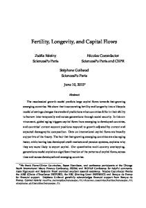
Figures 1 and 2 illustrate properties of the model solution.11 Figure 1 shows how the real option value of being a potential mother varies with the value of the underlying asset (the expected lifetime utility gain of motherhood). The curves represent the relationship 1, 12 and 120 months before the expiration date of the option (i.e. menopause), which is assumed to be known by all agents. The 45 degree line plots the gain in value from motherhood net investment costs. The tangency point between this line and each of the three curves are the childbearing thresholds in terms of expected lifetime utility gain. For T − t = 0, the investment rule is simply to choose motherhood if the expected gain net of costs is larger than zero. For younger women with more time remaining, we see that the threshold may be much higher than the expected gain itself, because the option leaves the agent with a value of waiting one period to make the decision. Because the option 11

Dixit and Pindyck (1994, pp.167-173) illustrates a solution of a similar model with infinite horizon in continuous time.

9

value can never be less than zero, the increased chance of highly favorable and highly non-favorable outcomes implied by a longer horizon increases the option value and the fertility threshold. A corresponding effect can be seen in Figure 2 where higher levels of uncertainty imply a higher option value of postponing childbearing, which increases the individual’s inaction range. If a peer’s childbearing generates a positive social externality the expected gain from motherhood will increase, potentially beyond the threshold where childbirth becomes optimal in which case fertility rate in the peer group goes up. If the social externality is negative, fertility in the rest of the group will decrease.12 Figure 2 illustrates how social influences may be affected by the level of uncertainty, σ. The tangency points show that increased uncertainty increases the size of the inaction region, requiring larger shifts to the value differentials for childbearing to become optimal. Thus, in this model coworkers childbearing are less influential under higher uncertainty.13 In our finite horizon setting, Figure 1 also show how the inaction region becomes smaller as t approaches T . Just like increased uncertainty, more time to maturity increases the upside potential of future option values while the downside potential is constant at zero, giving more incentive to wait and see. Thus, social influences should be weaker for women with longer time until the option to have a child expires. We explore these implications to see if the strength of the peer effect varies with the degree of uncertainty, and how it varies with the time left until the end of the fertile period. Since the identification of peer effects using observational data is difficult, we first describe our empirical strategy and data in detail. 12

It is worthwhile to note that out of all coefficients estimated below, negative point estimates are rare and in such cases they are almost never significant. This indicates that if the effects are driven by social influences, it seems as if positive externalities dominate in our setting. 13 This effect is recognized in the investment literature both theoretically (c.f Hassler (1996)) and empirically (c.f. Bloom et al. (2007))

10

3

Empirical design

The simple model outlined in the previous section is operationalized for the empirical analysis in the following way. The individual fertility decision is modeled as a function of co-workers’ past childbearing using a conditional linear probability model in discrete-time. The model can be thought of as a linear approximation of a proportional hazard model allowing for timevarying covariates, non-parametric duration dependence and time period effects (Allison, 1982).14 Our baseline specification is: Yijtc = αt + β1 (Any co-worker had a child within 12 months)ijtc + β2 (Any co-worker had a child within 13-24 months)ijtc

(5)

+ β3 (Any co-worker had a child within 25-36 months)ijtc Xijtc λ + Cijtc δ + ηθ + εijtc where the dependent variable Yijtc indicates whether employee i in workplace j had a child in calendar month c at duration month t. αt is a vector of month of duration dummies that non-parametrically control for the fact that the baseline hazard of childbearing varies dramatically over the life cycle (as seen in Figures A2 and A3). The variables “Any co-worker had a child within 12, 13-24 or 25-36 months” are indicators for whether a co-worker had a child within 12, 13-24 and finally 25-36 months prior to month c.15 14

We have also re-estimated the model using a Maximum Likelihood (complementary log-log) estimator. This provided similar results which are available upon request. 15 The variable “Any colleague had a child within twelve months” counts from t − 1 to t − 12. Hence, by construction, the dummy takes on the value of zero if the colleague gave birth to a child in the same month as the individual. This implies that we avoid the possibility that two colleagues having a child together show up as one of them responding to the other. It is important to note that peer effects may arise not only from whether any co-worker recently had a child, but also from the share of co-workers who did have a child. Empirically, since we focus on small and medium-size workplaces, this is not going to make much of a difference. In the robustness checks we do, however, provide evidence on this from regressions where we interact the baseline exposure variables with a dummy indicating if more than one co-worker gave birth to a child within the same time period.

11

Xijtc is a vector of individual background characteristics (marriage status and education), Cijtc is a vector of co-worker and workplace background characteristics such as the previous number of children among co-workers, age distribution, gender and educational attainments, and dummies controlling for establishment size in ten-worker intervals. ηθ is a vector of yearx monthx regionx industry dummies aimed to capture common macro shocks at the region-industry level that influence fertility decisions (for example, variation in the regional unemployment rate). Hence, we compare childbearing outcomes among employees in workplaces in the same year, month, three-digit industry and region with and without co-workers who recently had a child.16 Finally εijtc is the error term. The reported standard errors are adjusted for correlated errors at the workplace level.17 16

The three-digit industry classification is fairly detailed. In the education sector, it distinguishes between primary school, secondary school, higher education, and vocational school/adult education. In the manufacturing industry, it distinguishes e.g. between production of rubber or plastic goods. In the hotel and restaurant industry, it distinguishes between hotels, restaurant, camping, bar, and catering businesses. See http://www.foretagsregistret.scb.se/sni/040115snisorteradeng.pdf for full details. 17 The baseline empirical strategy follows the spirit of Kuziemko (2006) with some important modifications. Kuziemko (2006) estimates linear probability models and include individual fixed effects to identify the impact of sibling’s childbearing on individual childbearing. Duration dependence is controlled for using age in year dummies and indicators for whether the woman had a child within either of the previous three years. In order to estimate the individual fixed effects model she implicitly assumes that there are no differences in the baseline hazard between first and second births. She finds that the probability of having a child within the first 24 months after the birth of a sibling’s child increases by 17% on average. We do not include individual fixed effects since it is unlikely to help identify the effects of interest. In a hazard model framework, the closest equivalent of controlling for individual fixed effects is to exploit variation in the timing of treatment across multiple spells to allow for individual-specific heterogeneity (c.f. Lancaster, 1990; van den Berg 2000). When we can expect that the baseline hazard follows a reasonably similar pattern across spells, controlling for the common baseline hazard across spells is likely to capture important unobserved determinants of the timing of exit. While this approach may be reasonable when it concerns e.g. unemployment or sickness absence spells, as clearly displayed in Figures A2 and A3, the baseline hazards of having the first and second child are very different. Also see footnote 19 for a related discussion of workplace level fixed effects.

12

The main parameters of interest in equation (5) are β1 , β2 and β3 . The estimates of these parameters intend to capture the dynamic impact of co-workers’ recent fertility decisions on the likelihood of childbearing in a specific month. Our main analysis focuses on how co-workers’ childbearing affects the timing of first births since the variation in timing is largest for these births, but also because to be in the sample of individuals for whom we could estimate the time between first and second, one must have had a first birth. However, we also report estimates for higher order births. We estimate equation (5) for women under risk of having her first, second and third child separately using OLS.18 For first births, duration dependence is controlled for by “months since age 20” - specific indicator variables up until the first birth (or until censoring) and, for higher order births, the number of months from the previous birth. Note that the combination of the duration dummies (months since age 20) and calendar time effects also accounts for general cohort effects.

3.1

Threats to identification

The parameters of interest in equation (5) are identified under the assumption that the timing of co-workers’ childbearing is uncorrelated with omitted variables affecting individual childbearing, after controlling for age (in months) effects, calendar time-industry-region effects and other time-varying individual and co-worker characteristics. When could this assumption be violated? Changes in labor market conditions could change the individual’s and the co-workers’ fertility decisions simultaneously. Much of this variation in labor market conditions will be controlled for by the yearx monthx regionx industry dummies. However, firm level specific shocks that change the probability of childbearing among all co-workers, but not workers in other firms in the same industry and region, could also violate our key identifying assumption. In addition, if workers 18

During our observation period, higher order births are relatively uncommon.

13

sort into workplaces based on unobserved characteristics, e.g. childbearing preferences, we may find a spurious correlation between the childbearing of co-workers and the focal worker. Even though we are controlling for many important co-worker characteristics related to the timing of childbearing (average number of children, share in fertile ages, share close in age (±4 years), share of co-workers with college education, share females, share married) as well as occupational sorting and transitory unobserved shocks at the industry-regional level, individuals may still end up in the same workplace and have children at approximately the same time for unobserved reasons, despite the fact that they are not directly influenced by each other.19 To get a first sense of the potential severity of these basic and general concerns, we exploit the difficulty of anticipating exactly when conception takes place and the longitudinal data to form predictions about how the estimates of β1 , β2 , and β3 should behave if omitted factors are important. To see this clearly, suppose that two co-workers independently start trying to conceive at the same time (e.g. due to a change in firm policy). Due to the partly random nature of timing of conception, some will conceive sooner than others. However, calculations in Kuziemko (2006) suggest that the probability that individuals who start trying to conceive at the same time will end up having children more than six months apart is only around 14%. This implies that if unobserved common shocks are causing a spurious correlation between co-workers fertility decisions, we expect the strongest 19 A simple but unfeasible path to follow in order to try to control for workers’ sorting would be to add workplace fixed effects to equation (5). However, considering that we have a panel only stretching over 8 years and that we include lagged dependent variables for up to 36 months (which would be what the ”‘co-worker had a child”’ dummies would be characterized as in a within-workplace analysis) the workplace fixed effects estimates would, as is well known, be severely downward biased using an OLS estimator (Nickell, 1981). An alternative way of solving this problem would be to aggregate the data to the workplace level and then use a Arellano-Bond GMM estimator. But since an important focus of our analysis is to study in which way peer effects operate in relation to individual characteristics, we instead focus on other ways of ensuring that the peer effects are not simply driven by endogenous sorting of workers across workplaces.

14

effect to show up during the first twelve-month period after the birth of a co-workers child and then decline (i.e. β1 > β2 > β3 ). If instead the estimates simply reflect endogenous sorting of workers with similar fertility timing preferences across workplaces, we expect the timing of co-workers’ childbearing to be irrelevant. To make this clear, suppose that workers conceive independently of each other (i.e. no social influence) with some given probability each month. Then, since there is an equal chance of having a co-worker who gave birth within 12, 13-24, and 25-36 months, we would expect that β1 = β2 = β3 . In the following sections, we will see that our estimates do not match either of these predictions. We also assess the identifying assumptions using what we call “placebo peers”. We re-estimate the model in equation (5), but instead of focusing on the impact of the true co-workers, we check whether the childbearing behavior in three alternative groups of individuals also affects the fertility decisions of the focal worker. The placebo co-workers we consider are: i FIRM-LEVEL CO-WORKERS: These workers are employed in the same firm, region (21 regions), and two-digit industry, but not in the same workplace as the focal worker. ii FUTURE CO-WORKERS: This placebo peer group consists of future co-workers of the female employees in our sample that switch workplaces during the eight-year observation window.20 iii SIBLINGS OF CO-WORKERS: This placebo peer group is likely to share many of the co-workers’ observed and unobserved characteristics. They have experienced similar upbringings and might therefore have formed similar preferences for the timing of childbearing. These three placebo peer groups are likely to share many of the unobserved 20

To ensure that we capture actual job switchers, we restrict the sample to women who switch jobs only once during the observation period and we require that the individual is observed for at least two years before and after the change in jobs.

15

determinants of the timing of childbearing and experience similar unobserved shocks as the focal worker and the true co-workers. However, a priori, we do not expect to find a similar effect from childbearing in any of these placebo peer groups on the focal worker unless i) the baseline peer effect simply reflects a spurious correlation induced by unobserved factors that affect the timing of childbearing, or ii) they are directly influencing the focal worker. However, note that it is conceivable that the childbearing of siblings could influence the focal worker via the fertility decisions of the actual co-worker. In this case, we would expect the effect to show up after the additional lag it takes for first the co-worker and then the focal worker to react. Alternatively, if the sibling, the co-worker and the focal worker do not affect each other at all, but just share unobserved determinants of the timing of childbearing or if the sibling and the focal worker directly influence each other, we would expect to find a spurious placebo co-worker effect that follows the same pattern as the baseline results. Note that none of the placebo peer groups are perfect in isolation in the sense that they are not expected to share the exact same type of unobserved determinants or experience the same types of time varying unobserved shocks as the focal worker. However, they are imperfect in different ways. Hence, jointly they provide a strong test against the alternative spurious correlation hypothesis.

4

Data

The data we use come from the IFAU-database that contains various administrative registers covering the entire Swedish population aged 16-65. In addition to detailed individual background characteristics (LOUISE), the data contains firm and workplace identifiers (RAMS). From the “multigeneration” register, we add data on the full history of births as well as the month of birth of each child. This allows us to construct our measure of

16

co-worker fertility and our binary outcome variable; whether the focal worker gave birth to a child in a given month or not. We restrict the analysis to female workers aged between 20 and 44, employed in a workplace with less than 50 employees.21 We focus on women first of all because their fertility cycle is well-defined, but also because childbearing among women is associated with significant career interruptions. This restriction does not apply to co-workers. That is, the analysis looks at the impact of both male and female co-workers fertility on female workers fertility. The workplace size restriction is important since it allows us to focus on a well-defined peer group where interactions are likely to occur on a day-to-day basis. Our sample consists of 50 percent of the stock of women employed in 2004, followed for eight years back in time (1997-2004) 22 Hence, women are defined to be at the risk of childbearing from 1997 through the end of 2004 as long as they are observed in a workplace below 50 employees, until the month when they give birth or until the month they turn 45. To test whether our results are sensitive to our sampling procedure, we also construct a flow sample following cohorts of previously childless women from the year that they turn 20 in 1997-2004 (and thus become under risk of childbearing) until the month when they give birth. Since we require that the individuals should be working, we include them in our sample only in those years that we observe them in a workplace. This restriction implies that we will over sample individuals with stable employment. However, note that almost all women in Sweden remain in employment 21

The medical literature defines the childbearing age as the years falling between the age of 15 and 44. However, for simplicity, we restrict our sample to individuals who were aged above 20. Our choice is motivated by the fact that due to compulsory schooling in Sweden, it is very rare that individuals start working and having children before this age. In 2004, only 3.4 percent of Swedish women had their first child before their 20th birthday and the average age at first birth was 29 and 31 for women and men, respectively, in 2004 (National Board of Health and Welfare). 22 Since the data generating process requires that we expand each worker with the number of co-workers each year we have to restrict our sample to 50 percent of the women.

17

after giving birth to a child and hence, attrition is a minor concern. Relatively few workers hold multiple jobs. For those who do, we focus, for simplicity, on the workplace giving the primary source of earnings as the arena of social interaction. In addition, we always exclude workers who have zero or very low annual labor earnings (below the 10th percentile of the total annual labor earnings income distribution ). The cutoff, which corresponds to a yearly total labor income below 11000 SEK (1500 USD/1200 Euro) is applied to remove summer workers, very temporary workers or students working once a week etc.23 Without it co-workers is unlikely to be a good measure of a relevant peer group. The time until the pregnancy as well as the social influence of peers may be different for women having their first, second and third child, respectively. Therefore, we consider up to three fertility spells. For women without previous children, we define duration as the number of months from the age of 20 and up to their first birth (or censoring), and for mothers with one child (two children), duration is defined as the number of months from their previous child birth up to the second (third) or until they are censored. Individuals are followed from when they became fertile (had their previous child) and as long as they are of fertile age between 1997 and 2004. We combine this data with time varying information on the co-workers in the particular year, month and workplace and create indicators for whether any co-worker had a child in a specific month. We also add information on age structure, sex composition, the share of co-workers with college education, workplace size, number of children of the co-workers, region of work and the sector (public/private) and the three-digit industry of employment. Descriptive statistics for first-, second- and third-order spells are reported in Appendix A, Table A1. In our sample, mothers of first-born children are, on average, 27.6 years old and employed by workplaces with 18 employees.24 23

The threshold is computed each year and based on all employees in the labor market, both males and females. It is applied to focal women as well as to co-workers. 24 This is similar to the population average in Sweden during this time period.

18

The mean probability of having a child in a specific month is 0.005. The mean probability of having a second child is more than twice as high (0.011), reflecting that those who already have a child are much more likely to give birth to another child. The monthly probability of having a third child is only 0.002. These patterns reflect the two-child norm in Sweden. As shown in Figure A2 in Appendix A, the likelihood of childbearing for first-time mothers in our sample peaks around the age of 30. Figure A3 suggests that the probability of delivering a second child peaks after 28 months (2.3 years) and that most women (70 percent) had their second child within 6 years after their first child.

5 5.1

Main Results Baseline results

Column (1) of Table 1 shows the baseline estimates of the three β’s from equation (5), capturing the impact of co-workers’ childbearing on own fertility for women giving birth to their first child after controlling for duration dependence and year × month × region × industry cell fixed effects. The first, second and third rows report the estimates of β1 , β2 and β3 , i.e. the estimated impact of being exposed to a co-worker who had a child 1-12, 13-24 and 25-36 months earlier, respectively. The estimates are very robust across specifications. The estimates of β1 are small and not significantly different from zero but still precisely estimated. In contrast, the estimates of β2 and β3 indicate a positive (and declining) association between the focal worker’s childbearing and the past childbearing of her co-workers. The pattern of the parameters does not change significantly when adding controls for individual marital status and college education in column (2) or the co-worker and workplace controls in column (3). Together the estimates suggest that the co-workers’ fertility decisions primarily increase fertility with a lag of about one year. Evaluated at the baseline 19

probability of childbearing in a particular month, the fully specified model (column (3)) suggests that individuals are on average 9% (0.048/0.523) more likely to have their first child 13-24 months after the birth of a co-worker’s child. To put the estimates into perspective, first consider that for example Del Bono et al. (2012) find that women are about 10% less likely to have a child in the first couple of years after losing their job.25 The 12-24 month effect is also comparable to increasing the focal worker’s age by one (1) year in the age interval 20 through 30 or equivalently decreasing the focal worker’s age between ages 30 through 40. Moreover, the dynamic and consistent pattern across specifications gives a first indication that neither common unobserved shocks nor endogenous sorting are likely driving our results. As discussed in section 3.1 above, if unobserved common shocks were to induce individuals to start trying to conceive simultaneously, we would expect to find the largest effect within the first six months. We do not find any significant increase in childbearing until after twelve months. Similarly, the nonlinear pattern is difficult to reconcile with a simple endogenous sorting story. This is also supported by the fact that, conditional on the detailed yearx monthx regionx industry effects, adding an extensive set of individual, co-worker, and workplace controls hardly changes the pattern or the size of the point estimates at all. This could suggest that the empirically relevant sorting of workers based on childbearing preferences occurs at the 3-digit industry/region/time level or higher.

5.2

Robustness and validation checks

As a first specification check in column (1) of Table A3, we replace the three twelve-month indicators of interest with six six-month interval dum25 Interestingly, the magnitude of the social effect is furthermore very similar to those effects found in recent studies also focusing on co-worker peer effects in general. For example, Mas and Moretti (2009); Falk and Ichino (2006); Ichino and Maggi (2000); Hesselius et al. (2009) all find co-worker peer effects which are in the vicinity of our estimates, but for very different outcomes.

20

mies. These estimates are shown in Figure 3 (top), and suggest that the baseline specification indeed seems to do a good job in modeling the dynamic impact of co-workers’ childbearing. The main impact shows up after 13-18 months and then declines until it becomes insignificant after 31-36 months. Next we assess if increasing the dose of exposure matter by interacting the baseline variables of interest with dummy variables indicating if more than one co-worker had a child 1-12, 13-24 and 25-36 months ago. The estimates in column (2) provide a clear dose-response pattern of being exposed to the childbearing of several co-workers; the interaction terms are positive and of significant size. Controlling for additional births does, however, leave the baseline estimates essentially unchanged, suggesting that the main effect is not simply driven by exposure to many births. Therefore, we stick to the more parsimonious specification for the remainder of the analysis.26 Next we investigate whether sorting of workers based on e.g. the childfriendliness of the workplace is driving our results. Despite that our baseline model is likely to capture much of the selective sorting of this kind, it is possible that workers planning to have children systematically move to workplaces where childbearing is more frequent. As a first test of the validity of this concern, we split the sample with respect to worker tenure and report the results separately in columns (3) and (4) of Table A3. Comparing the estimates, we see that there are no major differences in the impact of peers on women with more and less than five years of tenure. If anything, the effect seems to be somewhat stronger for women with longer tenure, suggesting that sorting into establishments just before planning a pregnancy is not driving our results. The baseline estimates are based on a retrospective sample of women 26

We have also looked at the relationship between workplace size and the magnitude of the peer effect. The largest effects are found in the smallest workplaces and then decrease (although not necessarily monotonically with workplace size). The results from this exercise are available upon request.

21

observed working in 2004. In Table A4, we examine whether the results are sensitive to the choice of sampling procedure, by reestimating the baseline results using a flow sample instead. That is, for each year we select all women that become under risk (turn 20) and follow them until 2004 (as long as they are in a workplace with less than 50 employees). Effectively this implies that we limit our sample to women aged 20-27. To make the results comparable we construct two additional samples including women aged 28-36 and 37-44 respectively. Columns (1) to (3) reports the stock sample estimates for the same age groups (we will discuss these in more detail later). Due to the sampling procedure, women in the stock sample are older and therefore have higher baseline fertility rate. However, it is reassuring to see that the flow sample estimates confirm the pattern found in the baseline analysis. Putting the estimates in relation to the baseline fertility rate, the magnitudes are remarkably similar. It does not seem, therefore, that the estimates are driven by the choice of sampling method. Table 2 presents results from the placebo co-worker falsification exercise outlined in section 3.1 above. Column (1) reports the estimates for the first placebo peer group: firm co-workers, column (2) presents the results for the second placebo peer group: future co-workers, and column (3) shows the estimates for the third placebo peer group: co-workers siblings. It should be noted that the placebo tests restrict the samples to women working in private firms with more than one workplace in column (1), and to women who switch jobs in column (2).27 While the estimates for the true co-workers are highly similar to the baseline estimates, none of the three placebo co-worker regressions provide results that even vaguely resemble the main results.28 27

For comparison we also report the baseline estimates for the true co-workers’ childbearing in each of these sub-samples in Table A5. 28 One concern is that since the number of co-workers in the same firm can be much larger than the number of co-workers within the same workplace, we have also estimated the “same firm different workplace” regression only using firms that have less than a total of 50 employees. These estimates were very similar to the full placebo group sample estimates.

22

The only estimate that is significantly different from zero in any of the three placebo peer group regressions is the 25-36 month lagged effect in the co-workers’ sibling sample. To further assess this particular pattern, we estimated a model where we allowed co-workers’ siblings to affect the childbearing decisions of the focal worker in six-month intervals for up to 48 months. The results are presented in the lower panel of Figure 3. For comparison, we also show the six month interval estimates for the true co-workers in the upper panel. The parameter estimates are small and insignificant for the first 30 months after a co-worker’s sibling had a child, but there is an effect showing up with a lag of 31-36 months, which then fades out slowly. This suggests that the fertility decision spills over from the sibling of the co-worker via the co-worker to the focal worker. Finally, we allow the influence through a in equation (1) to vary with the degree of similarity between the co-workers in terms of gender, age, education and the number of previous children. A large sociological literature documents that individuals are much more likely to form social ties, and be influenced by peers who are more similar to themselves.29 The estimates are summarized in Figure A4. They suggest that similarity, social status, and prior experiences all play distinct roles in the social transmission of fertility decisions in social networks. The peer effect seems primarily to be driven by female co-workers and co-workers who are close in age (±4 years). College educated women seem to be affected by other college educated co-workers but not by those with a lower education. On the contrary, women without college education are similarly affected by both college educated co-workers and co-workers without college education. As such, the results bring additional support to our interpretation of the estimated effects as reflecting social influences rather than a spurious effect driven by unobserved common factors.30 29

For evidence of the relevance of homophily in social networks, c.f. McPherson et al. (2001); Currarini et al. (2009). 30 The only type of unobserved shocks that could explain these asymmetric parity and

23

5.3

Testing the model implications

i. Peer effects and uncertainty The first prediction of our model is that social influences should vary with the level of uncertainty about the value of becoming a mother. To test this, we re-estimate the baseline model with an added interaction term between the baseline indicators of whether a co-worker gave birth in the relevant time frame and two proxies of job-related uncertainty. We first try to capture the job-related uncertainty by using information on the tenure of the manager. We assume that, all else equal, working under a manager with long tenure is less uncertain than working under a manager with short tenure. The intuition is that in workplaces with a new manager the perceived risk of re-organizations, changes in firm policies, as well as managers’ less precise information about the worker’s productivity, and the new manager’s attitude towards childbearing, etc., lead to higher uncertainty about the future. However, as the manager’s tenure increases, this uncertainty is resolved because information about the manager’s attitudes and policies is revealed over time, as is information about e.g. the employees’ effort and productivity (Altonji and Pierret, 2001; Farber and Gibbons, 1996).31 education-specific peer effects patterns is workplace-specific shocks that only affect childbearing decisions among women with previous children (college education) but not women without children (without college education). On the contrary, unobserved shocks that affect childbearing decisions among women without previous children (without college education) must always also affect women with previous children (college education). The standard omitted variables that we are concerned about could lead to spurious correlations in fertility decisions within the workplace are unlikely to generate such asymmetric patterns. 31 To identify the manager, we use occupational codes and information on ownership. The data contains information on detailed occupational status for all establishments in the public sector and for a sample of private establishments. Information on ownership is available for all establishments in the economy. We identify the manager using the following hierarchical criteria: (1) Owner, (2) Top manager and (3) Middle manager. In case there are multiple managers at the same level, we assume that the manager is the individual with the highest wage. Manager tenure is defined as years at the workplace (truncated in 1985). Note that for sampling reasons, tenure is measured as the number

24

A potential concern when using manager tenure as a proxy for uncertainty is that high turnover firms may be overrepresented in firms with less tenured managers. If women sort into more or less stable workplace environments depending on their childbearing preferences, this could bias our results. To mitigate this concern, we add controls for individual and average co-worker workplace tenure in addition to the year×month×region×industry effects.32 As a second measure of uncertainty, we use the standard deviation of the workplace level churning rate over the observation period. The churning rate is a measure of the excess turnover of workers and restructuring, and has previously been used to measure industry or labor market uncertainty (c.f. Davis and Haltiwanger (1999)). Table 3, column (1) shows that the peer effect is significantly lower when uncertainty is high (new manager) compared to when it is low (tenured manager).33 A similar pattern, although less precisely estimated, is found when we include an interaction term between the peer effect and the variance of the workplace churning rate in column (2) (while controlling for the average workplace churning rate). In summary, the results in this section suggest that peers influences in fertility timing decisions matter most when job-related uncertainty is relatively low. This pattern is consistent with the model predictions that peer induced demand shocks for children should matter more when uncertainty about the net benefits of childbearing is lower. of years the current manager has been employed in the workplace. I.e. irrespective of whether he/she occupied the manager position for the whole period or not. Managers have an average tenure of 5.9 years (sd = 5.07). 32 However, the results are very similar even if we omit these additional controls. 33 The baseline estimates for the sample of workers for whom we can identify their manager’s tenure in the workplace are highly similar to the baseline results for the full sample.

25

ii. Peer effects and time to maturity The second prediction of the model is that the peer effect should become stronger as women approach the end of their fertile years. To test this, we simply divide the fertility phase of a woman’s life into an early (age 20-27), a primary (age 28-36) and a late (age 37-44) stage, and re-estimate the baseline model separately for women in these age groups. Columns (3)-(5) in Table 3 show that women in all age groups are influenced by their co-workers. However, consistent with the model, the peer effect is increasing in age: evaluated at the mean the estimates correspond to an increase in own childbearing of 7.3 percent in the early stage, 9.4 percent in the primary stage and 14.5 percent in the late stage of the fertility phase, as shown in Figure 4.34

5.4

Alternative explanations

i. Central planning and firms hiring policies If clustered timing of childbearing is costly for firms, it seems plausible that they may have developed policies encouraging women to space births (or take turns) to ensure an undisrupted conduct of business. Presumably any firm that hires women would make sure that if one (female) worker is not working as a result of having a child, another person would be available to temporarily replace that worker. This could potentially explain why we see stronger effects between more similar workers, since these are presumably better substitutes in the production process. However, this substitutability argument squares poorly with at least two 34

Since we do not have data on completed fertility for all workers in our sample, the distinction between pure timing effects and effects on completed family size is difficult. The fact that peers’ childbearing also influences women without previous children who are above their primary childbearing age does, however, indicate that social interactions may not only affect the timing of childbearing but also the decision of whether to have a child or not.

26

findings. First, assuming that leave-related costs are similar to the firm irrespectively of whether women are on leave with their first or second child, it is difficult to reconcile the substitutability story with the finding that influences from first to second time mothers are completely absent. Second, we find that low-skilled workers are clearly affected by the childbearing of their high-skilled co-workers (defined by education), who they are unlikely to replace in the production process. A final related concern is that the observed correlations in the timing of childbearing could be generated by firms’ hiring policies. Consider the case when firms use a staggered hiring strategy that generates a uniform distribution of worker tenure. Now combine this situation with workers preferring to have children just after some specific point in their career, for example after promotions. If promotions occur with regular intervals then it is possible to imagine a dynamic fertility-timing pattern similar to the one shown above. However, in some specifications presented above we do control for tenure at the plant and 3-digit industry dummies, which should account for much of this potential spurious variation in childbearing clustering. Again, it is difficult to explain the strongly heterogeneous peer effect patterns across different types of co-workers with such hiring practices. In an attempt to further try to rule out this possible alternative explanation, we investigated whether peers with longer or shorter tenure differentially influence women. If the peer effect is mechanically generated by the structure of hiring, this would result in a spurious association from peers with longer tenure to those with shorter workplace tenure. In contrast, if anything, we find that the peer influences are strongest from co-workers with lower tenure than the focal worker.35 35

One reason for why we see a larger peer effect from co-workers with shorter tenure could be due to a higher fraction of close-in-age co-workers in this group (29 compared to 15 percent). Although somewhat puzzling, the main point is that the tenure pattern is not consistent with a staggered hiring explanation without peer effects. These estimates are available upon request.

27

ii. Social learning Our model assumes that co-workers childbearing affects women’s fertility choices by changing the expected value of becoming mothers. An alternative explanation is that individuals resolve uncertainty about the value of childbearing by observing their co-workers childbearing experiences. Women may, for example acquire information from their female peers that reduce uncertainty about post-birth wage-profiles, career opportunities, or the possibility of combining children and work. However, from a standard social learning model, we would expect that women with more diffuse priors about the costs and benefits of having children should be more strongly influenced by their peers (see e.g. Bikhchandani et al. (1992), Banerjee (1992), Moretti (2011)). As shown in Table 4 we find that women who it seems reasonable to assume are better informed about the values and costs of children, are equally (or even more strongly) affected by their peers. Column (1) through (3) show that there are no marked differences in the magnitude of the peer effect (relative to their respective means) for women with no, one, or two previous children. Similarly, columns (4) and (5) show that women with long tenure (five years or more) are, if anything, more influenced by their peers than women with shorter tenure. Together these results speak in favor of social influences rather than social learning as the key underlying mechanism for the fertility peer effect.

6

Conclusions

In this study, we investigate how fertility decisions are transmitted in social networks. Specifically, we use unique matched employer-employee data and examine how recent births among co-workers affect the subsequent childbearing decisions among 140,000 Swedish women. We find that co-workers have a significant impact on the timing of childbearing. Consistent with the literature on the formation of social ties, same type peers are much more 28

influential than other type peers. We also show that the response to co-worker’s childbearing is weaker under higher uncertainty about the work-related costs of childbearing, and increases when women approach the end of their fertile ages. These results matches the predictions from our dynamic model of investments under uncertainty, where births among co-workers affect women through a shift in the expected value of becoming mothers. In contrast, there are no marked differences in the magnitude of the peer effect for women with differing precision in the prior about the costs and benefits of childbearing. These results together suggest that social influences rather than social learning is the key underlying mechanism in the current context. That social influences seems to be the dominant underlying mechanisms behind the fertility peer effects could suggest that policies that aim to reduce individuals uncertainty about the consequences of childbearing in order to increase fertility (for example through information programs, parental leave laws, subsidized childcare etc.), also unintendedly may result in larger fluctuations in the fertility rate by generating stronger peer effects.

29

References Allison, P. (1982). “Discrete-time Methods for the Analysis of Event Histories.” Sociological Methodology. Altonji, J. G., and Pierret, C. R. (2001). “Employer learning and statistical discrimination.” The Quarterly Journal of Economics, 116 (1), 313–350. Andersson, G. (1996). “Childbearing Trends in Sweden 1961-1997.” European Journal of Population, 15, 1–24. Arrow, K. J. (1968). “Optimal Capital Policy with Irreversible Investment.” In J. N. Wolfe (Ed.), Value, capital and growth papers in honor of Sir John Hicks, Edinburgh: Edinburgh University Press. Banerjee, A. V. (1992). “A simple model of herd behavior.” The Quarterly Journal of Economics, 107 (3), 797–817. Behrman, J. R., Kohler, H.-P., and Watkins, S. C. (2001). “The Density of Social Networks and Fertility Decisions: Evidence from South Nyanza District, Kenya.” Demography, 38, 43–58. Bernanke, B. (1983). “Irreversibility, Uncertainty, and Cyclical Investment.” The Quarterly Journal of Economics, 98 (1), 85–101. Bertola, G. (1988). “Irreversible Investment.” Massachusetts Institute of Technology doctoral thesis, re-printed in Research in Economics, 52, 3– 37. Bikhchandani, S., Hirshleifer, D., and Welch, I. (1992). “A theory of fads, fashion, custom, and cultural change as informational cascades.” Journal of Political Economy, 100 (5), pp. 992–1026. Bloom, N., Bond, S., and van Reenen, J. (2007). “Uncertainty and Investment Dynamics.” Review of Economic Studies, 74, 391–415. Currarini, S., Jackson, M. O., and Pin, P. (2009). “An Economic Model of Friendship: Homophily, Minorities and Segregation.” Econometrica, 77 (4), 1003–1045.

30

Dahl, G. B., Løken, K. V., and Mogstad, M. (2012). “Peer effects in program participation.” Working Paper 18198, National Bureau of Economic Research. Davis, S. J., and Haltiwanger, J. (1999). “On the Driving Forces behind Cyclical Movements in Employment and Job Reallocation.” American Economic Review, 89 (5), 1234–1258. Del Bono, E., Weber, A., and Winter-Ebmer, R. (2012). “Clash of Career and Family: Fertility Decisions after Job Displacement.” Journal of the European Economic Association, 10 (4), 659–683. Dixit, A., and Pindyck, R. S. (1994). Investment Under Uncertainty. Princeton: Princeton University Press. Durlauf, S. N., and Walker, J. R. (1998). “Social Interactions and Fertility Transitions.” mimeo, University of Wisconsin at Madison. Easterlin, R. A. (1975). “An Economic Framework for Fertility Analysis.” Studies in Family Planning, 6, 54–63. Falk, A., and Ichino, A. (2006). “Clean Evidence on Peer Effects.” Journal of Labor Economics, 24 (1), 39–57. Farber, H. S., and Gibbons, R. (1996). “Learning and wage dynamics.” The Quarterly Journal of Economics, 111 (4), 1007–1047. Fern´andez, R., and Fogli, A. (2006). “Fertility: The role of culture and family experience.” Journal of the European Economic Association, 4 (2-3), 552– 561. Fern´andez, R., and Fogli, A. (2009). “Culture: An empirical investigation of beliefs, work, and fertility.” American Economic Journal: Macroeconomics, 1 (1), 146–77. Feyrer, J. (2011). “The us productivity slowdown, the baby boom, and management quality.” Journal of Population Economics, 24 (1), 267–284. Freeman, R. (1979). “The Effect of Demographic Factors on Age-Earnings Profiles.” Journal of Human Resources, 14 (3), 289–318.

31

Glaeser, E., Sacerdote, B., and Scheinkman, J. (2003). “The Social Multiplier.” Journal of the European Economic Association, 1 (2-3), 345–353. Goldin, C., and Katz, L. F. (2012). “The most egalitarian of all professions: Pharmacy and the evolution of a family-friendly occupation.” Granovetter, M. S. (1995). Getting a Job: A Study of Contacts and Careers. Chicago: University of Chicago Press, Chicago, 2nd edn. Guryan, J., Kroft, K., and Notowidigdo, M. J. (2009). “Peer effects in the workplace: Evidence from random groupings in professional golf tournaments.” American Economic Journal: Applied Economics, 1 (4), 34–68. Hassler, J. (1996). “Variations in risk and fluctuations in demand: A theoretical model.” Journal of Economic Dynamics and Control, 20 (6-7), 1115– 1143. Herr, J. L., and Wolfram, C. (2009). “Opt-Out” Rates at Motherhood Across High-Education Career Paths: Selection Versus Work Environment.” NBER Working Paper No 14717. Hesselius, P., Johansson, P., and Nilsson, P. (2009). “Sick of your Colleagues Absence?” Journal of the European Economic Association, 7 (2-3), 583– 594. Higgins, M., and Williamson, J. G. (2002). “Explaining Inequality the World Round: Cohort Size, Kuznets Curves, and Openness.” Southeast Asian Studies, 40 (3), 268–302. Hoem, J. (1990). “Social Policy and Recent Fertility Change in Sweden.” Population and Development Review, 16, 735–748. Hotz, V. J., Klerman, J., and Willis, R. J. (1997). “The Economics of Fertility in Developed Countries.” In M. R. Rosenzweig, and O. Stark (Eds.), Handbook of Population and Family Economics, 275–347, New York: Elsevier. Ichino, A., and Maggi, G. (2000). “Work Environment and Individual Background: Explaining Regional Shirking Differences in a Large Italian Firm.” The Quarterly Journal of Economics, 115 (3), 1057–1090.

32

Ioannides, M. Y., and Loury, L. D. (2004). “Job Information Networks, Neighborhood Effects, and Inequality.” Journal of Economic Literature, 42 (4), 1056–1093. Iyer, S., and Velu, C. (2006). “Real Options and Demographic Decisions.” Journal of Development Economics, 80 (1), 39–58. Kato, T., and Shu, P. (2009). “Peer effects, social networks, and intergroup competition in the workplace.” Working Papers 09-12, University of Aarhus, Aarhus School of Business, Department of Economics. Katz, L., and Murphy, K. M. (1992). “Changes in Relative Wages, 1963-1987: Supply and Demand Factors.” The Quarterly Journal of Economics, 107, 35–78. Keim, S., Kl¨arner, A., and Bernadi, L. (2009). “Who is Relevant? Exploring Fertility Relevant Social Networks.” Max-Planck-Institut f¨ ur demografische Forschung Working Paper 2009-001. Kohler, H.-P. (1997). “Learning in Social Networks and Contraceptive Choice.” Demography, 34 (3), 369–383. Kohler, H.-P. (2001). Fertility and Social Interaction: An Economic Perspective. Oxford, United Kingdom: Oxford University Press. Kuziemko, I. (2006). “Is Having Babies Contagious? Estimating Fertility Peer Effects Between Siblings.” Mimeo, Yale University, June. Lyngstad, T., and Prskawetz, A. (2010). “Do siblings fertility decisions influence each other?” Demography, 47 (4), 923–934. Manski, C. F. (1993). “Identification of Endogenous Social Effects: The Reflection Problem.” Review of Economc Studies, LX, 531–542. Manski, C. F., and Mayshar, J. (2003). “Private Incentives and Social Interactions: Fertility Puzzles in Israel.” Journal of the European Economic Association, 1 (1), 181–211. Mas, A., and Moretti, E. (2009). “Peers at Work.” American Economic Review, 99 (1), 112–145.

33

McDonald, R., and Siegel, D. R. (1986). “The Value of Waiting to Invest.” The Quarterly Journal of Economics, 101, 707–727. McPherson, M., Smith-Lovin, L., and Cook, J. M. (2001). “Birds on a Feather: Homophily in Social Networks.” Annual Review of Sociology, 27 (415), 444. Moffitt, R. (2001). “Policy Interventions, Low-Level Equilibria, and Social Interactions.” In S. Durlauf, and P. Young (Eds.), Social Dymanics, Cambridge, MA: MIT Press. Montgomery, M. (1991). “New Evidence on Unions and Layoff Rates.” Industrial and Labor Relations Review, 44 (4), 1991. Montgomery, M., and Casterline, J. (1996). “Social Networks and the Diffusion of Fertility Control.” Policy Research Division Working Paper no. 119, New York: The Population Council. Moretti, E. (2011). “Social learning and peer effects in consumption: Evidence from movie sales.” The Review of Economic Studies, 78 (1), 356–393. Munshi, K., and Myaux, J. (2006). “Social norms and the fertility transition.” Journal of Development Economics, 80 (1), 1–38. Murphy, K. M., and Welch, F. (1992). “The Structure of Wages.” The Quarterly Journal of Economics, 107 (1), 285–326. Nickell, S. (1981). “Biases in dynamic panel data models with fixed effects.” Econometrica, 49, 1417–1426. Pindyck, R. (1988). “Irreversible Investment, Capacity Choice, and the Valuation of the Firm.” American Economic Review, 79, 969–85. Ranjan, P. (1999). “Fertility Behavior under Income Uncertainty.” European Journal of Population, 15, 25–43. Riksf¨ors¨akringsverket (2004). “Flexibel f¨or¨aldrapenning- Hur mammor och pappor anv¨ander f¨or¨aldraf¨ors¨akringen och hur l¨ange de ¨ar f¨or¨aldralediga.” RFV Analyserar 2004:14. Socialstyrelsen (2005). “Reproduktiv h¨alsa i ett folkh¨alsperspektiv.” Epidemiologiskt centrum, Stockholm. 34

Weinberg, B. (2007). “Social Interactions and Endogenous Association.” NBER Working Paper No 13038. Welch, F. (1979). “Effects of cohort Size on Earnings: The Baby Boom Babies’ Financial Busts.” Journal of Political Economy, October, 65–97. Wilde, E., Batchelder, L., and Ellwood, D. T. (2010). “The Mommy Track Divides: the Impact of Childbearing on Wages of Women of Differing Skill Levels.” NBER Working Paper 16582.

35

Tables and Figures Figure 1: Option value and time to maturity

Note: Model solution for β = 0.995, σ = 0.2 and µ = 0.

36

Figure 2: Option value and uncertainty

Note: Model solution for β = 0.995, T − t = 120 and µ = 0.

37

Figure 3: Spill-over effects between networks The impact of co-workers’ childbearing (top) and co-workers’ siblings’ childbearing (bottom).

38

Figure 4: Peer influences at different stages of the life-cycle

39

Table 1: Baseline estimates Any co-worker had a child within: 12 months 13-24 months 25-36 months Controls: Married

(1)

(2)

(3)

0.001 (0.007) 0.050*** (0.007) 0.016** (0.007)

0.002 (0.007) 0.050*** (0.007) 0.015** (0.007)

0.003 (0.007) 0.048*** (0.007) 0.011 (0.007)

1.184*** (0.016) -0.087*** (0.008)

1.183*** (0.017) College education -0.087*** (0.007) Total no of children of all co-workers 0.003*** (0.000) Share fertile co-workers 0.025 (0.016) Share close-in-age co-workers 0.071*** (0.018) Share female co-workers 0.084*** (0.014) Share married co-workers -0.015 (0.017) Share co-workers with college education -0.004 (0.016) Duration dummies Yes Yes Yes Calendar time× Ind.×Region dummies Yes Yes Yes Individual characteristics Yes Yes Establishment characteristics Yes Mean Y 0.523 0.523 0.523 R2 0.044 0.047 0.047 Observations 5,575,497 5,575,497 5,575,497 Notes: *,** and *** denote statistical significance at the 10, 5 and 1 percent level, respectively. Standard errors robust for clustering at the workplace level are shown in parentheses. The level of analysis is the individual-month. Calendar time is defined at the Y ear × M onth level. Industry is defined at the 3-digit level and the region is the county. For readability all coefficients have been multiplied by 100.

40

Table 2: Placebo co-workers (1) Same firm, different workplace Any co-worker had a child within: 12 months

(2) Future co-workers

(3) True co-workers’ siblings

0.015 -0.003 0.005 (0.025) (0.020) (0.007) 13-24 months -0.015 0.015 0.011 (0.025) (0.020) (0.007) 25-36 months 0.010 0.000 0.031*** (0.025) (0.020) (0.007) Duration dummies Yes Yes Yes Calendar time dummies Yes Yes Yes Individual char. Yes Yes Yes True co-work. char. Yes Yes Yes Placebo co-work. char. Yes Yes Yes Mean dependent variable 0.503 0.58 0.523 Observations 1,066,052 729,767 5,403,084 Notes: *,** and *** denote statistical significance at the 10, 5 and 1 percent level, respectively. Standard errors robust for clustering at the workplace level are shown in parentheses. The level of analysis is the individual-month. Calendar time is defined at the Year×Month level. Individual characteristics include civil status and a dummy for college education. Workplace characteristics include establishment size dummies in intervals of ten employees, the regional (county/year) unemployment rate where the workplace is located, the number of previous children in the workplace and the share of fertile, close-in-age, female, married and college-educated co-workers. The specification in column (2) additionally controls for firm size using nine dummies (2-9, 10-19, 20-29, 30-39, 40-49,50-99,100-199, 200-499, > 499 employees). For readability all coefficients have been multiplied by 100.

41

Table 3: Testing for social influences: uncertainty and time to maturity Uncertainty Time to maturity New vs. High/low Early: Primary: Late: old variability age age age manager in excess 20-27 28-36 37-44 turnover (1) (2) (3) (4) (5) Any co-worker had a child within: 12 months 0.020 -.020 -0.004 -0.009 -0.013 (0.020) (0.020) (0.008) (0.025) (0.020) 13-24 months 0.087*** 0.053*** 0.030*** 0.087*** 0.043** (0.020) (0.016) (0.008) (0.019) (0.020) 25-36 months 0.043* 0.028* 0.007 0.032* 0.033 (0.020) (0.016) (0.008) (0.019) (0.020) High uncertainty× Any co-worker had a child within: 12 months -0.006 -0.033 (0.037) (0.023) 13-24 months -0.079** -0.028 (0.033) (0.022) 25-36 months -0016 -0.033 (0.034) (0.023) Mean dependent variable 0.51 0.52 0.41 0.92 0.30 Duration dummies Yes Yes Yes Yes Yes Calendar time×Ind.×Region Yes Yes Yes Yes Yes Individual char. Yes Yes Yes Yes Yes Workplace char. Yes Yes Yes Yes Yes Observations 921,655 2,001,654 3,838,904 1,324,836 409,657 Notes: *,** and *** denote statistical significance at 10, 5 and 1 percent level respectively. Robust standard errors clustered at the workplace level are shown in parentheses. Column (1) measures uncertainty by an indicator for whether the manager has less than 4 years of tenure. Column (2) measures uncertainty by an indicator for whether the standard deviation of the workplace churning rate is above the median. The sample in column (1) consists of women in plants where the manager is identified. For computational reasons, the sample in column (2) is based on a 50 percent random sample of the total. All regressions include the same controls as the baseline (Table 1). Columns (1) and (2) include individual workplace tenure (0, 1-2, 3-4, 5-10, >10 years). In addition, column (1) includes 5 workplace age categories (0, 1-2, 3-4, 5-10, >10) and average tenure among the co-workers. For readability all coefficients have been multiplied by 100.

42

Table 4: Test of the social learning hypothesis Precision of prior: Precision of prior: Number of previous children: Workplace tenure: No One child Two Short Long children children tenure tenure (1) (2) (3) (4) (5) Any co-worker had a child within: 12 months 0.001 0.029 0.022 -0.001 0.029 (0.012) (0.028) (0.028) (0.007) (0.021) 13-24 months 0.047*** 0.151*** 0.040* 0.044*** 0.059*** (0.011) (0.025) (0.022) (0.007) (0.021) 25-36 months 0.024* 0.104*** 0.040* 0.011* 0.040* (0.011) (0.024) (0.008) (0.007) (0.021) Mean dependent variable 0.523 1.105 0.202 0.523 0.523 Duration dummies Yes Yes Yes Yes Yes Time×Ind.×Region eff. Yes Yes Yes Yes Yes Individual char. Yes Yes Yes Yes Yes Workplace char. Yes Yes Yes Yes Yes Observations 5,573,497 2,015,434 3,729,137 4,559,220 1,014,177 Notes: *,** and *** denote statistical significance at 10, 5 and 1 percent level respectively. Robust standard errors clustered at the workplace level are shown in parentheses. Long tenure is defined as having five years tenure or longer with the current employer. All coefficients have been multiplied by 100 to reflect percentage point changes.

43

A

Appendix material

Figure A1: Total fertility rate, 1900-2003, Source: Socialstyrelsen (2005)

44

Figure A2: Smoothed baseline hazard of first births

Figure A3: Smoothed baseline hazard of second births

45

Figure A4: Increase in the probability that an employee gives birth 13-24 months after a same-type/different-type co-worker. The estimated effects are evaluated at the mean monthly childbirth probability along with the 95% confidence intervals reported. For full results, see Appendix Table A6.

46

Table A1: Descriptive statistics Sample:

First birth Mean Sd

Second birth Mean Sd

Third birth Mean Sd

Had a child in current month Age College education

0.005 27.6 0.38

0.011 32.5 0.31

0.002 35.3 0.31

Number of children of co-workers Share fertile co-workers Share close in age co-workers Share female co-workers Establishment size Public sector Private sector Observations Individuals

20.5 18.9 0.67 0.25 0.23 0.20 0.65 0.29 18.2 12.5 0.27 0.45 0.73 0.45 5,575,497 139,020

0.072 5.4 0.49

47

0.105 5.1 0.46

23.6 20.2 0.62 0.25 0.20 0.18 0.66 0.30 18.1 12.6 0.34 0.47 0.66 0.47 2,015,434 60,534

0.045 4.3 0.46

25.6 20.8 0.59 0.25 0.20 0.17 0.67 0.31 18.2 12.4 0.40 0.49 0.60 0.49 3,730,264 73,518

Table A2: Descriptive statistics for true and placebo peer groups Sample:

Age Total # of children Female Fertile High edu. Married

Private firms with multiple workplaces True: Placebo: Same firm Same firm same different workplace workplace 35.3 36.2 (7.3) (6.4) 18.5 1,178 (16.4) (2196) 0.64 0.64 (0.27) (0.26) 0.69 0.66 (0.22) (0.18) 0.58 0.57 (0.25) (0.20) 0.35 0.36 (0.22) (0.18)

This peer had a child within 12 months 0.39 0.81 (0.49) (0.40) 13-24 0.42 0.82 months (0.49) (0.39) 25-36 0.42 0.82 months (0.49) (0.38) Obs. 1,066,052 1,066,052

Job switchers

All

True: Current co-work.

Placebo: Future co-work.

True: All co-work

Placebo: Co-work. siblings

37.6 (7.1) 20.3 (18.6) 0.66 (0.29) 0.64 (0.24) 0.30 (0.28) 0.41 (0.24)

36.1 (7.0) 19.9 (18.5) 0.65 (0.29) 0.63 (0.23) 0.32 (0.28) 0.39 (0.24)

36.7 (7.6) 20.5 (18.9) 0.65 (0.29) 0.65 (0.24) 0.31 (0.28) 0.38 (0.24)

38.2 (8.0) 19.1 (17.9) 0.49 (0.21) 0.57 (0.24) 0.27 (0.22) 0.36 (0.22)

0.34 (0.47) 0.38 (0.49) 0.37 (0.48) 730,356

0.39 (0.49) 0.40 (0.49) 0.38 (0.49) 730,356

0.36 (0.48) 0.39 (0.49) 0.37 (0.48) 5,575,497

0.36 (0.48) 0.36 (0.48) 0.34 (0.47) 5,385,787

48

Table A3: Specification checks Sample: Any co-worker had a child within: 1-6 months 7-12 months 13-18 months 19-24 months 25-30 months 31-36 months 12 months 13-24 months 25-36 months

(1) Baseline

(2) Baseline

(3) < 5 years of tenure

(4) ≥ 5 years of tenure

0.002 (0.008) 0.043*** (0.008) 0.013 (0.008)

-0.001 (0.007) 0.044*** (0.007) 0.011 (0.007)

0.029 (0.021) 0.059*** (0.021) 0.040* (0.021)

0.007 (0.008) 0.017** (0.008) 0.050*** (0.008) 0.028*** (0.008) 0.017** (0.008) 0.005 (0.008)

Multiple births: 12 months 0.024** ×1(> 1 birth) (0.012) 13-24 months 0.030*** ×1(> 1 birth) (0.01) 25-36 months 0.001 ×1(> 1 birth) (0.011) Duration dummies Yes Yes Yes Yes Calendar time × Industry Yes Yes Yes Yes × Region dummies Individual char. Yes Yes Yes Yes Workplace char. Yes Yes Yes Yes Mean Y 0.523 0.523 0.523 0.523 Observations 5,575,497 5,575,497 5,575,497 5,575,497 Notes: *,** and *** denote statistical significance at the 10, 5 and 1 percent level, respectively. Standard errors robust for clustering at the workplace level are shown in parentheses. The level of analysis is the individual-month. Calendar time is defined at the Y ear × M onth level. Industry is the defined at the 3-digit level and region is the county. Individual characteristics include civil status and a dummy for college education. Workplace characteristics include establishment size dummies in intervals of ten employees, the number of previous children in the workplace and the share of 49 fertile, close-in-age, female, married and college educated co-workers. 1(> 1 birth) is a dummy variable equal to 1 if at least two co-workers gave birth to a child during the previous ≤12, 13-24 and 25-36 months. For readability, all coefficients have been multiplied by 100.

Table A4: Stock vs. flow sample (1)

(2)

(3)

Early Primary Late (age 20-27) (age 28-36) (age 37-44) A: RETROSPECTIVE STOCK SAMPLE (baseline) Any co-worker had a child within 12 months -0.004 -0.009 -0.013 (0.008) (0.025) (0.020) 13-24 months 0.030*** 0.087*** 0.043** (0.008) (0.019) (0.020) 25-36 months 0.007 0.032* 0.033 (0.008) (0.019) (0.020) Mean dependent variable 0.41 0.92 0.30 Observations 3,838,904 1,324,836 409,657 B: FLOW SAMPLE (robustness check) Any co-worker had a child within 12 months -0.000 0.008 0.008 (0.005) (0.012) (0.000) 13-24 months 0.015*** 0.090*** 0.035*** (0.005) (0.012) (0.000) 25-36 months 0.013*** 0.014 0.027*** (0.004) (0.012) (0.000) Mean dependent variable 0.22 0.951 0.348 Observations 5,517,344 3,425,985 1,100,862 Duration dummies Yes Yes Yes Time×Ind.×Region eff. Yes Yes Yes Individual char. Yes Yes Yes Workplace char. Yes Yes Yes Notes: *,** and *** denote statistical significance at the 10, 5 and 1 percent level, respectively. Standard errors robust for clustering at the workplace level are shown in parentheses. The estimates reported in the upper panel is based on the (baseline) retrospective sample of women working in 2004 and is the same as in Table . The estimates in the lower panel is based on a flow sample of women entering the sample in 1997 or the first time they become under risk of having their first child and followed as long as they are working until 2004 or until they have their first child (see section 5 for a more detailed description). The level of analysis is the individual-month. Calendar time is defined at the Yearx Month level. Industry is defined at the 3-digit level and the region is the county. Individual characteristics include civil status and a dummy for college education. Workplace characteristics include establishment size dummies in intervals of ten employees, the number of previous children in the workplace and the share of fertile, close-in-age, female, married and college educated coworkers. For readability all coefficients have been multiplied by 100.

50

51

(1) True Same firm, same workplace

(2) Placebo Same firm, different workplace

(3) True Contemporary co-workers

(4) Placebo Future co-workers

(5) Placebo The true co-workers’ siblings

0.012 0.015 0.026 -0.003 0.005 (0.016) (0.025) (0.021) (0.020) (0.007) 13-24 months 0.067*** -0.015 0.072*** 0.015 0.011 (0.015) (0.025) (0.021) (0.020) (0.007) 25-36 months 0.019 0.010 0.032 0.000 0.031*** (0.016) (0.025) (0.021) (0.020) (0.007) Duration dummies Yes Yes Yes Yes Yes Calendar time dummies Yes Yes Yes Yes Yes Individual char. Yes Yes Yes Yes Yes True co-work. char. Yes Yes Yes Yes Yes Placebo co-work. char. No Yes No Yes Yes Mean dependent variable 0.503 0.503 0.58 0.58 0.523 Observations 1,066,052 1,066,052 729,767 729,767 5,403,084 Notes: *,** and *** denote statistical significance at the 10, 5 and 1 percent level, respectively. Standard errors robust for clustering at the workplace level are shown in parentheses. The level of analysis is the individual-month. Calendar time is defined at the Year×Month level. Individual characteristics include civil status and a dummy for college education. Workplace characteristics include establishment size dummies in intervals of ten employees, the regional (county/year) unemployment rate where the workplace is located, the number of previous children in the workplace and the share of fertile, close-in-age, female, married and college-educated co-workers. The specification in column (2) additionally controls for firm size using nine dummies (2-9, 10-19, 20-29, 30-39, 40-49,5099,100-199, 200-499, > 499 employees).

Any co-worker had a child within: 12 months

Peer group

Table A5: Placebo co-workers

52

(1) Female

(2) Close in age

(3) College education

(4) No college education

(5) No prev. children

(6) One prev. child

(7) Two prev. children

Any co-worker had a child within: 12 months 0.007 -0.031** 0.001 -0.035** 0.001 0.020 -0.007 (0.010) (0.008) (0.015) (0.016) (0.012) (0.019) (0.006) 13-24 months 0.016 0.009 0.011 0.063*** 0.047*** 0.023 0.009 (0.011) (0.008) (0.014) (0.017) (0.011) (0.019) (0.005) 25-36 months 0.000 -0.014* 0.005 -0.021 0.024** -0.009 0.007 (0.011) (0.008) (0.014) (0.017) (0.011) (0.019) (0.005) This type of co-worker had a child within: 12 months -0.000 0.088*** -0.005 0.052*** 0.003 0.029 0.022 (0.012) (0.012) (0.019) (0.017) (0.013) (0.028) (0.028) 13-24 months 0.047*** 0.107*** 0.058*** -0.011 0.000 0.151*** 0.040* (0.012) (0.012) (0.018) (0.018) (0.012) (0.025) (0.022) 25-36 months 0.0026** 0.096*** 0.042** 0.034** -0.009 0.104*** 0.040** (0.012) (0.012) (0.018) (0.017) (0.011) (0.024) (0.019) Duration dummies Yes Yes Yes Yes Yes Yes Yes Calendar time dummies Yes Yes Yes Yes Yes Yes Yes Individual char. Yes Yes Yes Yes Yes Yes Yes Workpl. char. Yes Yes Yes Yes Yes Yes Yes Mean dependent variable 0.523 0.523 0.562 0.498 0.523 1.105 0.202 Observations 5,575,497 5,575,497 2,140,535 3,432,418 5,575,497 2,015,434 3,729,137 Notes: *,** and *** denote statistical significance at the 10, 5 and 1 percent level, respectively. Standard errors robust for clustering at the workplace level are shown in parentheses. The level of analysis is the individual-month. Calendar time is defined at the Year×Month level. Individual characteristics include civil status and a dummy for college education. Workplace characteristics include establishment size dummies in intervals of ten employees, the regional (county/year) unemployment rate where the workplace is located, the number of previous children in the workplace and the share of fertile, close-in-age, female, married and college-educated co-workers. The specification in column (2) additionally controls for firm size using nine dummies (2-9, 10-19, 20-29, 30-39, 40-49,5099,100-199, 200-499, > 499 employees). For readability, all coefficients have been multiplied by 100.

SAMPLE

Table A6: Heterogeneous effects: gender, age and birth order