Boosting with pairwise constraints Changshui Zhang ,Qutang Cai ,Yangqiu Song State Key Laboratory on Intelligent Technology and Systems, Tsinghua National Laboratory for Information Science and Technology (TNList), Department of Automation, Tsinghua University, Beijing 100084, China

Abstract In supervised learning tasks, boosting can combine multiple weak learners into a stronger one. AdaBoost is one of the most popular boosting algorithms, which is widely used and stimulates extensive research efforts in the boosting research community. Different from supervised learning, semi-supervised learning aims to make full use of both labeled and unlabeled data to improve learning performance, and has drawn considerable interests in both research and applications. To harness the power of boosting, it is important and interesting to extend AdaBoost to semi-supervised scenarios. Moreover, in semi-supervised learning, it is believed that incorporating pairwise constraints such as side-information is promising to obtain more satisfiable results. However, how to extend AdaBoost with pairwise constraints remains an open problem. In this paper, we propose a novel framework to solve this problem based on the gradient descent view of boosting. The proposed framework is almost as simple and flexible as AdaBoost, and can be readily applied in the presence of pairwise constraints. We present theoretical results, show possible further extensions, and validate the effectiveness via experiments. Key words: Boosting, pairwise constraints, classifier ensemble, semi-supervised learning, gradient descent boosting

1 Introduction In supervised learning, Boosting [1] is a meta-algorithm that can create a single strong learner from a set of weak learners. Most boosting algorithms iteratively learn weak learners with respect to a distribution over training data and combine them with appropriate weights as a final strong classifier. The crucial steps in these boosting algorithms are their methods of weighting training data and hypotheses. AdaBoost [2] is one of the most popular algorithms in boosting. Although simple, AdaBoost is able to combine weak learners into a rather strong one. Experiments on real-world data [3] shows that AdaBoost has excellent performance, and is not Preprint submitted to Elsevier

16 July 2009

easy to overfit the data. Interestingly, the weak learners in AdaBoost have to be only slightly better than a random guess, which gives great flexibility to the choice of the weak classifier. Due to its simplicity, flexibility, and excellent power, AdaBoost has therefore gained popularity among practitioners, and has been extensively used and extended in many applications, such as text categorization [4], speaker detection [5], face detection [6], and cost-sensitive classification [7]. Semi-supervised learning [8], which makes use of both labeled and unlabeled data, has drawn considerable attentions recently. In many practical tasks, unlabeled training examples are often readily available but labeled data are fairly expensive to obtain. Therefore, it is important to take the most out of the labeled and unlabeled data. Compared with supervised learning, semi-supervised learning algorithms utilize useful observations extracted from labeled and unlabeled data to obtain a better classification performance in classification tasks [9,10], and to reach more satisfiable results in clustering scenarios [11–13]. One way to characterize useful observations for semi-supervised learning is via pairwise constraints, which can be used to model the relationships between instances. A pairwise constraint between two instances describes whether they should belong to the same or different classes (or clusters). Pairwise constraints have been successfully used in semi-supervised clustering [11,12,14–17] and in semisupervised classification [18–20]. It suggests that appropriately incorporating pairwise constraints is hopeful to further improve the performance of learning algorithms. We note that most of existing approaches using pairwise constraints only focus on developing specific algorithms. For example, the constrained K-means algorithm [15] adjusts the cluster memberships to comply with the prescribed constraints; the algorithms in [16,17] are designed to use the pairwise constraints in the prior probabilistic models for data clustering; the frameworks in [19,20] directly model the decision boundary. However, it is often the case that we already have a specifically designed basic learning algorithm, and we only need a meta-learning algorithm like AdaBoost to enhance its performance. Moreover, although there are some semi-supervised boosting classification algorithms [21–25], these methods do not make use of pairwise constraints. For example, the approaches in [21,22] attempt to maximize the objective functions derived from certain kinds of classification confidence, while the algorithms in [23–25] make use of the geometry of data manifolds. To our best knowledge, a general semi-supervised framework for incorporating pairwise constraints into boosting classifiers is still absent. In this paper, we propose a general framework to use both label information and pairwise constraints. We take the gradient descent approach to boosting [26,27] and derive the solution to our framework. As we will show in this paper, this method will generate promising results compared to the state-of-the-art boosting algorithm and can be extended analogously. The remainders of this paper are organized as 2

follows. In Section 2, we formulate the basic problem in this paper. In Section 3, we present a brief review of AdaBoost as well as its gradient descent treatment for our further study. In Section 4 and Section 5, we propose a new surrogate function, develop the gradient boosting procedure, and study its properties. In Section 6, we demonstrate a specialization of the boosting method and validate our framework via experiments. We conclude this paper in Section 7.

2 Problem formulation Let X and H denote the feature space and the set of weak learners, respectively. Since a multi-class problem in boosting can be converted into binary classification forms [28], we hence only consider binary classification problems with labels {+1, −1}. Let the labeled training data, L, be the instances x1 , · · · , xl with known labels y1 , · · · , yl . Let the unlabeled data, U, be the instances xl+1 , · · · , xl+u . Without additional confusion, we abbreviate xi ∈ L by i ∈ L, and abbreviate xi ∈ U by i ∈ U . Throughout this paper, we will use sgn(·), I(·) and span(H) as the sign function, the indicator function, the ensemble learner space based on H, respectively. The output of the weak learners in H is restricted to class labels, i.e., {+1, −1}. 2.1 Pairwise constraints Similar to the must-link and cannot-link in semi-supervised clustering [8], there are also two types of pairwise constraints in classification scenarios: the sameclass and different-class constraints. The same-class constraint between xi and xj requires that the labels assigned to xi and xj are the same, while the different-class constraint requires that the labels are different. We denote the sets of the prescribed same-class constraints and different-class constraints by S and D, respectively. We also let the whole set of constraints, C1 , · · · , Cn , be denoted as C (C = S ∪D). For a pairwise constraint Ck , we let i ∈ Ck represent that the constraint involves instance xi , and we denote the event that Ck is fulfilled by Ck = 1 (otherwise, Ck 6= 1). Note that it may be difficult to satisfy all the given constraints simultaneously, especially when there are potential conflicts within the prescribed constraints. Therefore, we will use soft constraints instead. For each constraint Ck , we introduce a cost ck when Ck is violated. Thus, in the ensemble problem with pairwise constraints, a natural objective is to seek an optimal ensemble classifier F that minimizes l X i=1

|

+

I(F (xi ) 6= yi ) {z

n X

k=1

}

|

empirical misclassification cost

ck I(Ck 6= 1), {z

}

constraint violation cost

3

(1)

which involves the cost of empirical misclassification and violating constraints. Remark 1 Note that we place no additional restrictions on C and ck ’s, thus bringing some flexibility: • Conflicts, redundancies and duplications are allowed among the constraints in C, since we only care about the total violation cost. • The instances involved in the constraints can be arbitrary. A constraint in C can be between a labeled instance and an unlabeled instance, or between two unlabeled instances. Since a constraint between a labeled instance and an unlabeled instance is equivalent to assign a (pseudo-)label to the unlabeled instance, without loss of generality, we will only consider constraints between unlabeled instances.

2.2 Examples

We now present two common examples in semi-supervised classification concerning pairwise constraints. (1) Smoothness assumption: The smoothness assumption, which is often considered in semi-supervised learning [8], is that if two instances are close to each other, the corresponding labels are likely to be the same. One feasible way to incorporate the smooth assumption is via designing the violation costs ci ’s: the closer the two nearby instances, the higher the corresponding violation cost of the same-class constraint. (2) Special instances: In some classification tasks, several special unlabeled instances are more interesting than others. Although their true labels are unknown, one can impose same-class and different-class constraints according to their similarity or dissimilarity. The decision boundary modeling problem below can serve as a more concrete example: The optimal decision boundaries are often unknown, and can be difficult to explicitly obtain due to modeling and computational difficulties. Moreover, it is almost impossible to explicitly specify the decision boundary for some classifiers (e.g., support vector machines with RBF kernels). However, it remains feasible to model the decision boundary using pairwise constraints. Note that two instances from different classes are always located on different sides of the true boundary. In other words, the true boundary is located between these two instances. Similar to the case where support vectors in SVMs determine the separating hyperplane, it is expected that the resulting classifier is likely to have a good decision boundary when the different-class constraints involving special data that are located near the correct boundary are satisfied. This is also the basic idea in [19]. 4

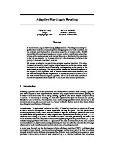
We present another example on how to construct pairwise constraints in practical applications, which is taken from a scenario of classifying people’s identities in surveillance video[13]. In this scenario, one can benefit from the inherent characteristics of video streams, such as the sequential continuity, to pose different types of constraints automatically or only with little human effort. For example, in Fig. 1, one can readily obtain the pairwise constraints with the aid of temporal relations: (1) two spatially overlapping regions extracted from temporally adjacent frames can be assumed to share the same labels (see Fig. 1(a)); (2) two regions appearing simultaneously in a frame cannot be labeled as the same (see Fig. 1(b)).

(a)

(b)

Fig. 1. Examples of pairwise constraints: (a) Same-class constraints from a single tracked sequence, (b) Different-class constraints between different regions in the same video frame.

3 AdaBoost and gradient descent boosting We briefly review AdaBoost as well as its gradient descent viewpoint [26] for the subsequent study. The gradient descent viewpoint for AdaBoost is useful for both devising new boosting algorithms (e.g., see [21,22]) and analyzing Boosting’s performance such as population theory [29], convergency [30] and consistency [31,32]. Let Ft be an ensemble classifier, which is a linear combination of t base classifiers, Ft (x) =

t X

αi fi (x),

(2)

i=1

where fi ’s are the base classifiers which output ±1 and t is the number of base classifiers used. A natural objective for the ensemble of classifiers is to minimize the empirical classification error of labeled training data, l X

I(Ft (xi ) 6= yi ),

i=1

5

(3)

which can be viewed as a special case of the objective function in (1) without the cost component for constraint violation. 3.1 Surrogate function Note that global minimization of (3) is a typical combinatorial optimization problem and is generally intractable [33]. AdaBoost uses a surrogate loss function instead of 0 − 1 loss used in (3), R(F ) ,

l X

exp(−yi F (xi )),

(4)

i=1

which is an upper bound of (3) since I(Ft (xi ) 6= yi ) ≤ exp(−yi F (xi )).

(5)

Although (4) is difficult to be globally optimized directly, R(F ) possesses the following ”good” properties for gradient optimization. With Ft−1 fixed, R(Ft−1 + αf ) possesses the following properties: (1) Differentiability: R(Ft−1 + αf ) is differentiable with respect to f . We denote the linear operator of the Gateaux derivative at Ft−1 in the direction of f by R0 (Ft−1 ; f ). R0 (Ft−1 ; f ) ,

l X ∂R(Ft−1 + αf ) |α=0 = − exp(−yi Ft−1 (xi )) × yi f (xi ). (6) ∂α i=1

The greedy descent direction for R(Ft−1 + αf ) at α = 0 is ft∗ , arg max f ∈H

= arg max f ∈H

(t−1)

where Di Pl

(t−1) i=1 Di

=

l X i=1 l X

yi f (xi ) exp(−yi Ft−1 (xi )) (t−1)

Di

I(f (xi ) = yi ) −

i=1

l X

(t−1)

Di

I(f (xi ) 6= yi ),

(7)

i=1

exp(−yi Ft−1 (xi )) Zt−1

and Zt−1 =

Pl

i=1

exp(−yi Ft−1 (xi )). Since

= 1, (7) can be reduced to arg min f ∈H

l X

(t−1)

Di

I(f (xi ) 6= yi ),

(8)

i=1

which can be carried out by learning the classifier with minimal error under P (t−1) (t−1) I(f (xi ) 6= yi ) by err(t) (f ) probabilities Di ’s. We also denote li=1 Di for later use. 6

(2) Convexity: for any fixed f , R(Ft−1 + αf ) is strictly convex and infinite differentiable with respect to α, and is globally minimized when ∂R(Ft−1 + αf ) = 0. ∂α

(9)

Thus, the optimal α can be analytically given by P

l 1 exp(−yi Ft−1 (xi ))I(sgn(f (xi )) = yi ) α = ln Pi=1 l 2 i=1 exp(−yi Ft−1 (xi ))I(sgn(f (xi )) 6= yi ) 1 1 − err(t) (f ) = ln . 2 err(t) (f ) ∗

(10)

3.2 Gradient boosting procedure The above two properties of R(F ) suggest that (4) can be optimized iteratively in an alternative optimization fashion: in each iteration, seek the optimal descent direction f ∗ , then choose the optimal step size α∗ along the direction of f ∗ , and add α∗ f ∗ to the ensemble. Following the steps in (6–10), the algorithmic procedure of AdaBoost can be summarized in Table 1. As in Table 1, AdaBoost employs an iterative procedure to produce a final classifier, which is a linear combination of weak hypotheses. At each stage of its algorithmic procedure, AdaBoost maintains a probability distribution on the examples, and then obtains an optimal weak learner under current probability settings. The weak learner is then used to update the distribution, and the hard examples receive higher probability. At the end of each iteration, the weak hypothesis is added to the linear combination to form the current hypothesis of the algorithm.

4 Surrogate function with pairwise constraints As a generalization of (3), the objective function (1) is also difficult to be minimized directly. To derive our boosting methods in the gradient descent boosting framework, we need a new surrogate function for (1) similar to the surrogate function (4) for (3). We require that the new surrogate function should share the differentiability and convexity properties of (4). This section aims to devise such a surrogate function. 4.1 A simple surrogate function First, we make the following observation as described in Lemma 1. 7

Table 1. Algorithmic Procedure of AdaBoost Input: Labeled data L. (0)

Initialization: Set weights Di = 1l on each instance xi . Iteration: Repeat for t = 1, 2, . . . , T : (t−1)

(a) Train weak learner ft∗ using weights Di

’s,

ft∗ = arg min err(t) (f ),

(11)

f ∈H

P (t−1) where err(t) (f ) = li=1 Di I(f (xi ) 6= yi ). (b) Compute the optimal weight αt∗ of ft∗ by (10): αt∗ =

1 1 − err(t) (ft∗ ) ln , 2 err(t) (ft∗ )

and the ensemble classifier of current iteration is F (t) = (c) Reweigh: update the probability setting of training data (t)

(t−1) −α∗t yi ft∗ (xi )

Di = Di

e

Output: output the final ensemble classifier F (T ) =

(12) Pt

∗ ∗ i=1 αi fi .

/Zt .

(13)

PT

∗ ∗ t=1 αt ft .

Lemma 1 Let F be the ensemble classifier, and suppose the pairwise constraint Ck involves two unlabeled instances, xi and xj . (1) If Ck is a same-class constraint, then I(Ck 6= 1) ≤ min{exp(−F (xi ))+exp(−F (xj )), exp(F (xi ))+exp(F (xj ))}. (14) (2) If Ck is a different-class constraint, then I(Ck 6= 1) ≤ min{exp(−F (xi ))+exp(F (xj )), exp(F (xi ))+exp(−F (xj ))}. (15) PROOF. (1) Note that I(Ck 6= 1) = I(sgn(F (xi )) 6= sgn(F (xj ))) and the right-hand side of (14) is always positive. We only need to show that the right-hand side of (14) is not less than 1 when sgn(F (xi )) 6= sgn(F (xj )). When sgn(F (xi )) 6= sgn(F (xj )), the values of F (xi ) and F (xj ) contain a positive value. Therefore,  exp(−F (x )) + exp(−F (x )) i j exp(F (xi )) + exp(F (xj ))

8

> exp(0) = 1 > exp(0) = 1.

(16)

By (16), the inequality (14) holds. (2) This can be proved in a procedure similar to (1).

2

According to Lemma 1, for each Ck ∈ C, we construct a mapping φk : span(H) → R+ by (1) If Ck is a same-class constraint, φk (F ) , min{exp(−F (xi )) + exp(−F (xj )), exp(F (xi )) + exp(F (xj ))}; (17) (2) If Ck is a different-class constraint, φk (F ) , min{exp(−F (xi )) + exp(F (xj )), exp(F (−xi )) + exp(F (xj ))}; (18) where xi and xj are the two instances involved in Ck . A qualitative comparison between (17–18) and (5) indicates that • The upper bound in (5) is greater than 1 when xi is misclassified, and tends to zero as F (xi ) increases when xi is correctly classified. • The upper bound in (17–18) is greater than 1 when Ck is violated, and tends to zero as F (xi ) and F (xj ) increase when Ck is satisfied. Lemma 1, (4) and (5) suggest that the following function in (19) can be used as a surrogate function for (1), Q(F ) =

l X

exp(−yi F (xi )) +

i=1

n X

ck φk (F ).

(19)

k=1

Remark 2 A comparison between Q(F ) and R(F ) gives the following immediate results: • The expression of R(F ) is simple in the sense that it is a linear combination of the exponential functions, which is convex and infinitely differentiable. The expression of Q(F ) is still simple, but it is not differentiable. • When ck ≡ 0, a.k.a. there is no constraints, Q(F ) = R(F ). Therefore, R(F ) is a special case of Q(F ). • If all labeled instances are correctly classified, as |F (xi )| tends to ∞ for all xi ’s, the risk R(F ) → 0. Similarly, if all labeled instances are correctly classified and all constraints are satisfied, as |F (xi )| tends to ∞ for all xi ’s, Q(F ) → 0. 4.2 Alternative formulation We have seen that the new surrogate function Q(F ) is a simple generalization of R(F ). However, for a fixed Ft−1 ∈ span(H) and variables α ∈ R, f ∈ H, un9

like R(Ft−1 + αf ) in (6–10), Q(Ft−1 + αf ) does not possess the differentiability and convexity properties, which prevents the usage of the gradient descent boosting framework. However, we observe that the two parts in min(·) in the definition of φ(·) possess these properties. In the following, we seek the way to utilize this observation to develop the gradient descent procedure for reducing (19). In the construction of φk (·) in (17–18), for each constraint Ck , we introduce auxil(1) (2) iary functions φk (·), φk (·) and φ˜k as in Definition 1. Definition 1 (Auxiliary functions) Suppose Ck involves xi and xj (i ≤ j). We (1) (2) define φk : span(H) → R+ and φk : span(H) → R+ as follows: (1) If Ck is a same-class constraint, (1)

(2)

φk (F ) , exp(−F (xi ))+exp(−F (xj )), φk (F ) , exp(F (xi ))+exp(F (xj )); (2) If Ck is a different-class constraint, (1)

(2)

φk (F ) , exp(−F (xi ))+exp(F (xj )), φk (F ) , exp(F (xi ))+exp(−F (xj )). Furthermore, we define another auxiliary function φ˜ : span(H) × [0, 1] → R+ , (1) (2) φ˜k (F, a) = a · φk (F ) + (1 − a) · φk (F ).

(20)

In Definition 1, φ˜k (F, a) is an extension of φk (F ), and it is readily seen that φk (F ) = min φ˜k (F, a). a

(21)

It can also be verified that the optimal a in (21), a∗k , arg min φ˜k (F, a),

(22)

a∈[0,1]

should take value in {0, 1}. Thus, intuitively, a∗k can be viewed as a selector for (0) (1) φk (F ) in {φk (F ), φk (F )}. With (20–22), we can reformulate (19) as the following. ˜ ; a1 , · · · , an ) : span(H) × [0, 1]n → R+ be defined as Lemma 2 Let Q(F ˜ ; a1 , · · · , an ) , Q(F

l X

exp(−yi F (xi )) +

i=1

Then,

n X

ck φ˜k (F, ak ).

˜ ; a1 , · · · , an ). Q(F ) = a min Q(F ,··· ,a 1

(23)

k=1

n

10

(24)

PROOF. By (21), l X

˜ ; a1 , · · · , an ) = min min Q(F a ,··· ,a a ,··· ,a 1

n

n

1

= =

l X i=1 l X

exp(−yi F (xi )) +

i=1

n X

ck φ˜k (F, ak )

k=1

exp(−yi F (xi )) + exp(−yi F (xi )) +

i=1

n X k=1 n X

ck min φ˜k (F, ak ) a k

ck φk (F )

k=1

= Q(F ).

2

˜ ; a1 , · · · , an ) Therefore, reducing Q(F ) for F ∈ span(H) is equivalent to reducing Q(F n for F ∈ span(H) and (a1 , · · · , an ) ∈ [0, 1] , i.e., min

F ∈span(H)

Q(F ) =

min

F ∈span(H) a1 ,··· ,an

˜ ; a1 , · · · , an ). Q(F

(25)

Moreover, like R(Ft−1 + αf ) in (6–10), with Ft−1 and a1 , · · · , an fixed, ˜ t−1 + αf ; a1 , · · · , an ) is differentiable with respect to f at α = 0. The lin(1) Q(F ear operator of the Gateaux derivative at Ft−1 and (a1 , · · · , an ) in the direction ˜ 0 (Ft−1 , a1 , · · · , an ; f ) for later use. of f is denoted by Q ˜ t−1 +αf ; a1 , · · · , an ) is convex and differentiable with respect (2) for fixed f , Q(F to α. ˜ ; a1 , · · · , an ) can also be decreased using the Therefore, with a1 , · · · , an fixed, Q(F alternate optimization technique, whence we will develop our boosting procedure.

5 Boosting with pairwise constraints In this section, we will derive in details the boosting algorithm from the gradient descent boosting framework, and study the risk bound during the boosting procedure. 5.1 Optimization method Like AdaBoost, we will employ an iterative alternative optimization procedure to ˜ ; a1 , · · · , an ), keeping one of F and (a1 , · · · , an ) fixed and optimizing reduce Q(F ˜ with respect to the other. Let F (t−1) , (a(n−1) ) be the values of F Q(·) , · · · , a(n−1) 1 n and (a1 , · · · , an ) in the previous iteration (the t−1-th iteration), respectively. 11

(t−1) ˜ (t−1) + α · • Step 1: keep (a1 , · · · , an ) fixed to (a1 , · · · , a(t−1) ) and reduce Q(F n (t−1) f ; a1 , · · · , a(t−1) ) with respect to F : We take the same procedure as AdaBoost n in (6–10), and we only need to seek a new α · f to add to the previously obtained Ft−1 . (1) Seek maximal descent direction:

˜ 0 (F (t−1) , a1(t−1) , · · · , a(t−1) ; f ). ft∗ = arg max −Q n f ∈H

(26)

(2) Choose the optimal step size along the direction of f ∗ : ˜ (t−1) + αf ∗ ; a(t−1) , · · · , a(t−1) ). αt∗ = arg min Q(F 1 n t α

(27)

Then the new F is F (t) = F (t−1) + αt∗ ft∗ . ˜ (t) ; a1 , · · · , an ) with respect to • Step 2: Keep F = F (t) fixed and optimize Q(F (t) a1 , · · · , an : By (21), the optimal a1 , · · · , a(t) n can be directly given by (t)

ak =

 1, 0,

if φ˜k (F (t) ) > φ˜k (F (t) ), otherwise. (1)

(2)

(28)

Compared with the minimization of the surrogate function of AdaBoost in (6–10), (t) the only new step introduced in (26–28) is the step for determining ak ’s. 5.2 Boosting procedure Having described necessary introduction and analysis, we are now in a position to develop the detailed boosting procedure. More specifically, we need to develop the detailed steps for (26) and (27). 5.2.1 Maximal descent direction In (26), ˜ (t−1) + αf ; a1 , · · · , a(t−1) ) ∂ Q(F n (t−1) ˜ 0 (F (t−1) , a(t−1) ; f ) = Q , · · · , a |α=0 1 n ∂α (t−1) l n X X ∂ exp{−yi (F (t−1) (xi ) + αf (xi )))} ∂ φ˜k (F (t−1) + αf, ak ) = |α=0 + ck |α=0 ∂α ∂α i=1 k=1 (t−1) l n X X ∂ φ˜k (F (t−1) + αf, ak ) (t−1) =− yi exp(−yi F (xi ))f (xi ) + ck |α=0 . (29) ∂α i=1 k=1 (t−1)

(t−1)

∂ φ˜ (F (t−1) +αf,a

)

k In (29), it suffices to consider k |α=0 . As in Definition 1, we as∂α (1) sume here that Ck involves xi and xj , i ≤ j. Note that both φ˜k (F (t−1) + αf ) and

12

(2) φ˜k (F (t−1) + αf ) can be unified as

exp{λ1 (F (t−1) (xi ) + αf (xi ))} + exp{λ2 (F (t−1) (xj ) + αf (xj ))},

(30) (t−1)

where λ1 , λ2 ∈ {±1} only depend on the constraint type of Ck . Since ak ∈ (t−1) (t−1) {0, 1}, φ˜k (F + αf, ak ) falls in the same set as in (30), and can be unified in the following form (t−1) φ˜k (F (t−1) +αf, ak ) =

X

(t−1),+

γk,m

(t−1),−

exp(−αf (xm )) + γk,m

exp(αf (xm )),

m∈{i,j}

(31) (t−1),+ (t−1),− (t−1) where γk,m , γk,m ≥ 0 are determined by ak and the constraint type of (t−1) Ck . For example, when Ck is a same-class constraint and ak = 1, we have (t−1),− γk,m = 0 and  exp(−F (t−1) (x )), i (t−1),+ γk,m = (t−1) exp(−F (xj )),

if m = i; if m = j. (t−1)

On the other hand, when Ck is a same-class constraint and ak (t−1),+ γk,m = 0 and  exp(F (t−1) (x )), i (t−1),− γk,m = (t−1) exp(F (xj )), (t−1),+

= 0, we have

if m = i; if m = j.

(t−1),−

(t−1),+

We extend γk,m and γk,m for convenience: when m ∈ / {i, j}, let γk,m (t−1),− and γk,m = 0. Then by (29) and (31),

=0

˜ 0 (F (t−1) , a(t−1) Q , · · · , a(t−1) ; f) 1 n

(32)

=−

l X

f (xi ){I(yi = +1)exp(−yi F (t−1) (xi ))} −

i=1

+

l X

l+u X

f (xi ) ·

i=l+1

f (xi ){I(yi = −1)exp(yi F (t−1) (xi ))} +

i=1

l+u X i=l+1

n X

(t−1),−

ck γk,i

k=1

f (xi ) ·

n X

(t−1),−

ck γk,i

.

k=1

By (32), the maximal descent direction in (26) can be thus obtained with the following steps: i) Assign weights and pseudo-labels: Let  I(y = +1)exp(−F (t−1) (x )), if i ∈ {1, · · · , l}, i i (t−1),+ hi , Pn (t−1),+  k=1 ck γk,i

,

otherwise,

 I(y = −1)exp(F (t−1) (x )), if i ∈ {1, · · · , l}, i i (t−1),− hi , Pn (t−1),−  k=1 ck γk,i

,

13

otherwise.

(33)

(34)

Pl+u (t−1),+

Note that we have

i=1

hi

+

Pl+u (t−1),− i=1

hi

= Q(F (t−1) ). Furthermore, let

(t−1),+

(t−1),+

Di

,

(t−1),−

hi hi (t−1),− , and D , . i Q(F (t−1) ) Q(F (t−1) )

(35)

(t−1),+

To each xi , we assign pseudo-label +1 with probability Di , and, at the (t−1),− same time, assign pseudo-label −1 with probability Di . The assignment approach is determined according to the base classifier. If the base classifier support weighted data, one can simply make the weights of xi with pseudo-label (t−1),+ (t−1),− +1 and −1 to be Di and Di , respectively. Otherwise, one can approximately construct new training data by randomly resampling from the original training data using the probability distribution given in (35), and then use them for training the base classifier . ii) Train the new base learner: By (33–35), the right-hand side in Equation (32) can be rewritten as −Q(F

(t−1)

)·

(l+u X

(t−1),+ Di f (xi )

−

i=1

)

l+u X

(t−1),− Di f (xi )

.

i=1

Therefore, Equation (26) can be converted into ft∗ = arg max f ∈H

= arg min f ∈H

l+u X

i=1 l+u X

(t−1),+

Di

f (xi ) −

l+u X

(t−1),−

Di

f (xi )

i=1 (t−1),+

Di

I(f (xi ) 6= +1) +

i=1

l+u X

(t−1),−

Di

I(f (xi ) 6= −1),(36)

i=1

where the last equality follows from the fact that f (xi ) ∈ {±1} and Pl+u (t−1),− = 1. Note that in (36), i=1 D l+u X

(t−1),+

Di

I(f (xi ) 6= +1) +

i=1

l+u X

(t−1),−

Di

Pl+u

I(f (xi ) 6= −1)

i=1

D(t−1),+ +

(37)

i=1 (t−1),+

(t−1),+

is the classification error of f under the probability law D1 , · · · , Dl+u , (t−1),− (t−1),− D1 , · · · , Dl+u with corresponding pseudo-labels. We also denote (37) by err(t) (f ). Therefore, ft∗ can be found by learning the classifier with minimal training error with the assigned probabilities and corresponding pseudo-labels.

5.2.2 Optimal step size When the new classifier ft∗ is found, we need to determine its weight. In (27), we ˜ (t−1) + αft∗ ; a(t−1) ) is convex with respect α. Hence , · · · , a(t−1) have seen that Q(F 1 n 14

the optimal αt∗ satisfies ˜ (t−1) + αf ∗ ; a1 ∂ Q(F t ∂α

(t−1)

, · · · , a(t−1) ) n

|α=α∗t = 0,

which gives that l+u X

(t−1),+

exp(−α∗ f ∗ (xi ))f ∗ (xi ) −

Di

i=1

l+u X

(t−1),−

Di

exp(α∗ f ∗ (xi ))f ∗ (xi ) = 0.(38)

i=1

By (38) and the fact that f ∗ (·) ∈ {±1}, l+u X

∗

e−α · ( ∗

(t−1),+

Di

i=1 l+u X

= eα · (

I(f ∗ (xi ) = +1) +

(t−1),+

Di

l+u X

i=1 l+u X

I(f ∗ (xi ) 6= +1) +

i=1

(t−1),−

Di

I(f ∗ (xi ) = −1))

(t−1),−

Di

I(f ∗ (xi ) 6= −1)).

i=1 ∗

∗

Therefore, we have e−α (1 − err(t) (ft∗ )) = eα err(t) (ft∗ ) and then αt∗ =

1 1 − err(t) (ft∗ ) ln . 2 err(t) (ft∗ )

(39)

5.2.3 Algorithmic procedure We summarize in Table 2 the boosting procedure with pairwise constraints, which we name by AdaBoost.PC. Though the above analysis for the development of AdaBoost.PC is somewhat complicated, the procedure of AdaBoost.PC is still simple. The comparison of AdaBoost.PC and AdaBoost is given as follows. Remark 3 (1) When there is no presence of pairwise constraints C, the steps in Table 2 are identical to that in Table 1. Thus, AdaBoost can again be viewed as a special case of AdaBoost.PC. (2) The methods for learning the base classifiers and determining their corresponding weights of AdaBoost.PC and AdaBoost are identical in essence. The main difference between Table 2 and Table 1 lies in the step for updating probabilities of the instances. AdaBoost is known to decrease its surrogate function R(F (t) ) throughout the iterations. We have similar results for AdaBoost.PC. Proposition 1 Throughout the iterations of AdaBoost.PC, the surrogate function Q(F (t) ) decreases. Moreover, ˜ (t) ; a(t−1) Q(F (t) ) ≤ Q(F , · · · , a(t−1) ) ≤ Q(F (t−1) ). 1 n 15

(42)

Table 2. AdaBoost.PC: Procedure for Boosting with Pairwise Constraints Input: Labeled data L, unlabeled data U and pairwise constraints C. Initialization: Let F (0) = 0. Assign each instance xi pseudo-label +1 with probabil(0),+ (0),− ity Di and pseudo-label −1 with probability Di , as in (35). Iteration: Repeat for t = 1, 2, . . . , T : (t−1),+

(a) Train weak learner ft∗ using weights Di corresponding pseudo-labels,

(t−1),−

’s and Di

’s together with the

ft∗ = arg min err(t) (f ),

(40)

f ∈H

P (t−1),+ (t−1),− where err(t) (f ) = l+u I(f (xi ) 6= +1) + Di I(f (xi ) 6= −1). i=1 Di ∗ ∗ (b) Compute the optimal weight αt of ft by (39): αt∗ =

1 1 − err(t) (ft∗ ) ln , 2 err(t) (ft∗ )

(41)

P and the ensemble classifier of current iteration is F (t) = ti=1 αi∗ fi∗ . (t),+ (c) Reweigh: update the probability setting for all pseudo label assignments, Di ’s (t),− and Di ’s. For each instance xi , (t) (t),+ (t),− (c.1) update ak , γk,i , γk,i by (28) and (31); (t),+

(t),−

(c.2) update probability Di for pseudo-label +1, and probability Di pseudo-label −1 by (33–35); P Output: output the final ensemble classifier F (T ) = Tt=1 αt∗ ft∗ .

for

PROOF. By step (a–b) in Table 2 (see also (26) and (27)) and Lemma 2, we have ˜ (t) ; a(t−1) ˜ (t−1) + αt∗ ft∗ ; a(t−1) Q(F , · · · , a(t−1) ) = Q(F , · · · ,a(t−1) ) 1 1 n n (t−1) ˜ (t−1) ; a1 , · · · , a(t−1) ) = Q(F (t−1) ). ≤ Q(F n

Moreover, by Lemma 2 and (28), we have (t) ˜ (t);a(t) ˜ (t) (t−1),· · · ,a(t−1) ). Q(F (t) ) = Q(F 1 ,· · ·,an ) ≤ Q(F ; a1 n

Therefore, the inequality (42) holds.

2

Proposition 1 guarantees the descent of Q(F (t)) in each iteration, and from this point of view, the initialization step in Table 2 is not crucial in the gradient descent framework and other initialization measures can be adopted as required. 16

5.3 Risk bound We present below an upper bound for risk function (1), which is analogous to Theorem 6 in [2]. Note that Theorem 1 is reduced to Theorem 6 in [2] when ck = 0, k = 1, · · · , n. Theorem 1 Suppose the base learners, f1∗ , · · · , fT∗ , generated in AdaBoost.PC have weighted training errors ε1 , · · · , εT (i.e., εt = err(t) (ft∗ )). Then the risk of the final classifier F (T ) in (1) is bounded above by (l +

n X

2ck )

T q Y

2 εt (1 − εt ).

(43)

t=1

k=1

PROOF. Since Q(F ) is an upper bound of (1), then when F (T ) is used as the classifier, the risk in (1) is upper bounded by Q(F (T ) ). Moreover, ˜ (t−1) + α∗ f ∗ ; a(t−1) Q(F , · · · , a(t−1) ) 1 t t n (t−1) Q(F ) =

l+u X

(t−1),+

Di

exp(−αt∗ ft∗ (xi )) +

i=1

= (1 − err

l+u X

(t−1),−

Di

i=1 (t−1)

∗ (ft∗ ))eαt

+ err

(t−1)

∗

exp(αt∗ ft∗ (xi )) q

(ft∗ )e−αt = 2 εt (1 − εt ),

t where the last equality follows from αt∗ = 21 ln 1−ε . By Proposition 1, we have εt

T q q Y Q(F (t) ) (T ) (0) ε (1 − ε ), and Q(F ) ≤ Q(F ) εt (1 − εt ). ≤ 2 2 t t Q(F (t−1) ) t=1

In (44), Q(F (0) ) = Q(0) = l +

Pn

k=1

2ck , and the conclusion then follows.

(44) 2

To understand the significance of Theorem 1, assume that for some ² > 0 , εt ≤ 0.5 − ² forq all t (i.e., ft∗ ’s are uniformly slightly better than random guessing). Then √ 2 we have 2 εt (1 − εt ) ≤ 1 − 4²2 ≤ e−2² , which means that the upper bound in (43) decreases exponentially fast with T .

6 Specialization and experiments We will show in this section that the ASSEMBLE algorithm [22], the winner in the 2001 NIPS Unlabeled Data Competition, can also be viewed as a special case of 17

AdaBoost.PC, and present experiments to illustrate the effectiveness of the boosting procedure.

6.1 The ASSEMBLE algorithm In the following, we will show an interesting fact that the ASSEMBLE algorithm [22] can also be covered by AdaBoost.PC. The significance of this fact is two-fold. Firstly, it indicates that AdaBoost.PC can be used as a more general framework for developing concrete boosting algorithms. Secondly, the effectiveness of ASSEMBLE demonstrated in [22] also validates the effectiveness of AdaBoost.PC. Moreover, the analysis below can also serve as an example for deriving concrete algorithms from AdaBoost.PC. The ASSEMBLE procedure of AdaBoost adopts the following surrogate function, QASSEM (F ) ,

l X i=1

|

exp(−yi F (xi )) {z

}

cost on labeled data

+

λ |

l+u X i=l+1

exp(−|F (xi )|), {z

(45)

}

cost on unlabeled data

where λ is a constant for the significance of cost on unlabeled data in the surrogate function. Intuitively, for unlabel instance xi , |F (xi )| can be viewed as the confidence of classifying xi as sgn(F (xi )). Thus, an ideal optimal F not only attempts to correctly classify labeled data but also needs to have good confidence on the unlabeled data, and the surrogate function (45) offers tradeoff between the labeled and unlabeled data. We restate the iteration procedure of ASSEMBLE in Table 3. After each iteration, the ASSEMBLE algorithm assigns each unlabeled instance one pseudo-label for the next iteration. It can be seen that the iterations are similar to those in AdaBoost, except that they introduce the step for updating pseudo-labels of the unlabeled data. To derive the ASSEMBLE algorithm from AdaBoost.PC, we should introduce constraints that lead to the same surrogate function. Since we impose no restriction on the instances involving in pairwise constraints, we can employ the following constraints: for each unlabeled instance xl+k , k = 1, · · · , u, we impose a same-class pairwise constraints on xl+k and xl+k (i.e., the two instances involved are identical) with corresponding violation cost ck = λ/2. By (17) and Definition 1, φk (F ) = min{2 exp(−F (xl+k )), 2 exp(F (xl+k ))} = 2 exp(−|F (xl+k )|), (1) (2) φ˜ (F ) = 2 exp(−F (xl+k )), and φ˜ (F ) = 2 exp(F (xl+k )). k

k

Plugging the values of φk (F )’s and ck ’s into Equation (19) gives the surrogate function (45). 18

Table 3. The ASSEMBLE iterations. (Repeat for t = 1, 2, . . . , T :) (t−1)

(a) Train weak learner ft∗ using weights Di

(t−1)

’s with (pseudo-)labels yi

,

ft∗ = arg min err(t) (f ),

(46)

f ∈H

where err(t) (f ) =

Pl+u i=1

(t−1)

Di

(t−1)

I(f (xi ) 6= yi

).

(b) Compute the optimal weight αt∗ of ft∗ by (10): αt∗ =

1 1 − err(t) (ft∗ ) ln , 2 err(t) (ft∗ )

and the ensemble classifier of current iteration is F (t) =

(47) Pt

∗ ∗ i=1 αi fi .

(c) Reweigh and relabel: (c.1) update the pseudo-label ( (t) yi

=

yi , sgn(F (t) (xi )),

xi ∈ L, xi ∈ U;

(c.2) update the probability setting of both labeled and unlabeled data ( (t) (t) e−yi F (xi ) /QASSEM (F (t) ), xi ∈ L, (t) Di = (t) (t) −y F (x ) (t) i λe i /QASSEM (F ), xi ∈ U.

(48)

(49)

We now show that the iterations in Table 2 for ASSEMBLE is the same as that in Table 3. In Table 2, using QASSEM (F ) as the surrogate function instead, (t)

(t),+

(t),−

step c.1 ak , γk,i , γk,i

(t)

can be directly computed by ak = sgn(F (t) (xl+k )),

 exp(−F (t) (x )), i (t),+ γk,i = 0,  exp(F (t) (x )), i (t),− γk,i = 0, (t),+

step c.2 Di

(t),+ Di

(t),−

and Di

xi ∈ U, and sgn(F (t) (xi )) = +1, otherwise, xi ∈ U , and sgn(F (t) (xi )) 6= +1, otherwise.

(50)

(51)

can be computed by  (t)   exp(−F (xi )),

i ∈ L and yi = +1, = 1/QASSEM (F (xi ))×λ exp(−F (xi )), i ∈ U and sgn(F (t) (xi )) = +1,   0, otherwise, (t)

(t)

19

(t),− Di

 (t)   exp(F (xi )),

i ∈ L and yi = −1, = 1/QASSEM (F (xi ))× λ exp(F (xi )), i ∈ U and sgn(F (t) (xi )) 6= +1,    0, otherwise. (t)

(t)

(t),−

(t),+

Observe that for each instance xi in L∪U , only one of Di and Di is nonzero. (t),− (t),+ Moreover, which one in {Di , Di } is nonzero depends solely on yi if xi is labeled, and on sgn(F (t) (xi )) if xi is unlabeled. Then the above calculations can be (t) simplified by assigning each xi one (pseudo-)label yi which indicates the pseudolabel with positive probability for xi , as given by (48). Thus, it can be readily veri(t),+ (t),− and Di are unified by (49) and step (a–b) in Table 2 is equivalent fied that Di to that in Table 3. Therefore, the procedure of AdaBoost.PC under the above constraints is equivalent to the ASSEMBLE algorithm. In addition, by Proposition 1, we obtain that the objective function is monotonously decreasing throughout the ASSEMBLE procedure. We can alsoqobtain an upper Q bound using Theorem 1 that QASSEM (F (T ) ) ≤ (l + 2λu) Tt=1 2 εt (1 − εt ). 6.2 Real-world data experiments As a special case, the experiments[22] concerning ASSEMBLE also validate the effectiveness of AdaBoost.PC. We also conduct new experiments on the boosting benchmark (available from http://ida.first.fraunhofer.de/projects/bench/benchmarks.htm, compiled by Gunnar R¨atsch) as supplementary to illustrate the effectiveness of our algorithms. Each data set consists of samples from two classes, and all the attributes are real values. The brief information of each dataset is described in Table 4. Table 4.Data sets used in experiments. Data Set Banana Breast-Cancer Diabetes Flare-Solar German Heart Image

Samples Attributes 5300 277 768 1066 1000 270 2310

2 9 8 9 20 13 18

Data Set Samples Attributes Ringnorm Splice Thyroid Titanic Twonorm Waveform

7400 3175 215 2201 7400 5000

20 60 5 3 20 21

Since decision stumps (one-level binary decision trees [34,35]) are typical weak classifiers that are simple to implement and can be combined into a fairly strong classifier by boosting [3], we use them as the base classifiers in the experiments. Moreover, we also use 8-node C4.5 decision trees [36], which are more complicated than decision stumps, as the base classifiers. 20

In each experiment, for each dataset, we randomly split the data points into three parts: labeled (L), unlabeled (U) and test (T ). The proportion of the test data T is fixed to 10% of the whole data, and the rest of the data, L ∪ U, are used for training. For each dataset, we run the experiments independently 100 times using four proportions (10%, 20%, 40%, 60%) of L∪U as the labeled data L, respectively. The pairwise constraints are generated through the following two steps: (1) Randomly split U into two equal parts, denoted by U1 and U2 . (2) For each instance x1 in U1 , find its nearest neighbor x2 in U2 . If x1 and x2 belong to the same class, then generate a same-class constraint between them, otherwise generate a different-class constraint. After the constraints are generated, the actual labels of the unlabeled data are dropped. In practical applications, the violation costs can be tuned by prior knowledge or cross-validation techniques. To simplify the experiments, we make the violation costs ck ’s be equal to a constant c, and fix the tradeoff between constraint vio1 lation cost and empirical misclassification cost in (1) to be 0.05 (i.e., let c = 20 l/n). In each experiment, we use the labeled data for the training of the base learners and AdaBoost, and use the labeled data together with the pairwise constraints on the unlabeled data for the training of the proposed algorithm. The boosting algorithms are run for 100 and 25 steps for decision stumps and C4.5 decision trees, respectively, (0) (0) without special care of overfitting. The initial starting points a1 , a2 , · · · , a(0) n for AdaBoost.PC are all set to be 0.5. The training results are tested on the test data T for calculating the misclassification error rates. Since the procedure of AdaBoost.PC is quite similar to that of AdaBoost, the CPU time used in AdaBoost and AdaBoost.PC is comparable in our experiments. The classification results with decision stumps and 8-node decision trees as the base classifiers are presented in Table 5 and Table 6, respectively. We also present results of the base classifiers and AdaBoost (using decision stumps and 8-node decision trees as the base classifiers, respectively) for comparison. When the proportions of the labeled data are small, we observe that the average error rates of AdaBoost.PC are lower than the other two algorithms in most cases. Moreover, a 95% confidence significance test corrected for multiple testing with the Bonferroni method also indicates that AdaBoost.PC also performs statistically better for most datasets. These indicate that taking pairwise constraints into account into boosting is very helpful for further reducing the classification error for small-size labeled data. As the size of the labeled data increases in the experiments, we also observe that incorporating the pairwise constraints may bring little benefit or even deteriorate the classification accuracy. It is interesting to investigate the factors that may affect the performance of AdaBoost.PC. We only mention a few briefly as follows: 21

• The choice of base learners used in AdaBoost.PC may largely affect the classification accuracy. For example, the testing accuracy of AdaBoost.PC on the banana dataset is reduced by 50%∼60% when using 8-node decision trees instead of decision stumps as the base learners. • We have conducted additional experiments to test the sensitivity of AdaBoost.PC to the initial starting points. We adopt two other methods for setting the starting (0) (0) points a1 , a2 , · · · , a(0) n as follows: · Method I: All the starting points are made to agree with the actual labels of the unlabeled data U. For example, for a same-class constraint involving xi and xj , let  1, the corresponding actual labels of i and j are +1 (0) ak =  0, otherwise.

· Method II: All the starting points are made to contradict the actual labels of the unlabeled data U. This method is the opposite of Method I. The other experimental settings remain unchanged. In our experiments, there is little statistical significance between the training results of these two initialization methods in most cases. However, for the image dataset and 40% of the labeled data using 100 decision trees, the testing error rates are 2.07±0.95 and 2.28±0.98 for Method I and II, respectively, where Method I also performs statistically better than Method II. • The method for generating pairwise constraints may also affect the classification accuracy. For the case of 10% of the labeled data with decision stumps as the base learners, we cast AdaBoost.PC only using the same-class constraints and the different-class constraints in the generated constraints, respectively. We observe that the error rate on the Diabetes dataset with the same-class constraints is 27.05 ± 5.35, and the error rate on the ringnorm dataset with the differentclass constraints is 5.60 ± 0.92. Both the results are statistically better than the corresponding results in Table 5.

6.3 Further possible generalizations An obvious advantage of the proposed boosting method is its flexibility inherited from AdaBoost. AdaBoost.PC can be applied with the presence of pairwise constraints whenever AdaBoost can be used in the corresponding supervised scenarios. A closer look at the derivation of AdaBoost.PC reveals that it still can be further generalized. We point out briefly two possible further generalizations for AdaBoost.PC. (1) General surrogate functions: The gradient descent framework in [26] provide a general way for devising boosting algorithms when the surrogate functions are given. The AdaBoost.PC framework can be generalized analogously. 22

Table 5. Experimental results with decision stumps Labeled Base

10% ADA

Banana 42.06 (2.47) 28.77 (2.53) B.Cancer 29.81 (7.51) 34.37 (8.59) Diabetes 30.36 (7.65) 28.45 (5.33) F.Solar 41.21 (10.69) 44.50 (11.70) German 31.00 (3.47) 30.42 (4.48) Heart 29.85 (10.15) 26.56 (9.33) Image 29.74 (4.63) 7.89 (2.11) Ringnorm 38.21 (1.36) 6.08 (1.03) Splice 24.58 (3.95) 9.61 (1.75) Thyroid 25.00 (9.57) 14.95 (9.91) Titanic 22.77 (2.42) 23.12 (2.41) Twonorm 33.51 (1.64) 3.91 (0.72) Waveform 23.53 (2.54) 12.46 (1.50) Win

1

0

Base

40% ADA

Labeled Banana B.Cancer Diabetes F.Solar German Heart Image Ringnorm Splice Thyroid Titanic Twonorm Waveform Win

41.37 (1.86) 28.96 (7.05) 26.70 (4.59) 37.71 (6.10) 30.06 (0.66) 26.96 (8.72) 27.74 (3.09) 38.07 (1.33) 23.10 (2.61) 22.91 (6.52) 22.50 (2.05) 32.93 (1.51) 23.21 (2.14) 0

APC 29.15 (2.44) 36.11 (8.69) 27.31 (5.34) 44.29 (13.51) 29.63 (4.28) 24.26 (9.21) 7.77 (2.18) 6.04 (1.00) 8.79 (1.61) 13.82 (7.67) 23.02 (2.46) 3.57 (0.64) 12.03 (1.56) 6 APC

28.52 (2.35) 28.88 (1.89) 28.96 (7.11) 28.19 (7.59) 24.39 (4.50) 24.29 (4.28) 39.79 (11.89) 39.43 (11.42) 25.72 (4.42) 25.58 (4.10) 21.52 (7.98) 20.70 (7.79) 4.84 (1.58) 5.28 (1.67) 5.11 (0.85) 5.21 (0.91) 6.84 (1.40) 6.61 (1.34) 7.91 (5.07) 7.27 (4.96) 22.32 (2.10) 22.32 (2.09) 3.39 (0.66) 3.29 (0.64) 11.30 (1.28) 11.55 (1.29) 3

1

Base

20% ADA

41.45 (2.11) 28.87 (2.25) 28.48 (6.55) 34.19 (10.37) 28.40 (5.43) 25.90 (5.72) 39.14 (10.28) 43.07 (12.29) 30.31 (1.33) 27.60 (4.04) 28.48 (8.60) 23.93 (9.23) 28.91 (3.85) 5.78 (1.61) 38.12 (1.31) 5.35 (0.77) 24.00 (3.59) 8.22 (1.43) 22.95 (7.38) 10.05 (6.47) 22.50 (2.05) 22.61 (2.30) 33.28 (1.70) 3.60 (0.68) 23.55 (2.35) 11.83 (1.41)

28.99 (2.02) 33.74 (9.36) 25.01 (5.15) 41.64 (11.53) 27.08 (4.10) 21.67 (8.33) 6.06 (1.83) 5.43 (0.84) 7.62 (1.38) 8.14 (6.24) 22.48 (2.14) 3.48 (0.62) 11.83 (1.49)

1

0

5

Base

60% ADA

APC

41.40 (1.90) 28.93 (7.02) 26.73 (4.11) 36.57 (3.70) 30.00 (0.00) 26.70 (8.64) 27.12 (2.37) 37.83 (1.39) 22.91 (2.17) 23.18 (6.11) 22.50 (2.05) 32.77 (1.75) 23.07 (1.91)

28.61 (2.05) 27.85 (6.65) 24.17 (4.68) 39.79 (11.59) 25.06 (4.22) 19.04 (7.79) 4.56 (1.66) 5.07 (0.84) 6.59 (1.53) 5.82 (4.79) 22.29 (2.02) 3.29 (0.63) 11.10 (1.44)

28.91 (1.83) 27.30 (6.96) 23.73 (4.44) 38.71 (10.80) 25.47 (4.43) 19.67 (7.36) 4.96 (1.67) 5.13 (0.85) 6.46 (1.36) 5.55 (4.94) 22.30 (2.04) 3.28 (0.64) 11.15 (1.40)

0

2

0

Experimental results, comparing the error rate of decision stumps (Base), AdaBoost (ADA), and our algorithm (APC). The standard deviations are also presented in the brackets. For each dataset, we put in emphasis the statistically significantly best algorithm. The last row counts the number of times each algorithm performs significantly best.

23

APC

Table 6. Experimental results with 8-node decision trees Labeled Base

10% ADA

APC

Banana 21.15 (3.02) 13.46 (1.78) 13.34 (1.67) B.Cancer 32.56 (8.61) 33.70 (8.40) 35.63 (8.22) Diabetes 30.56 (6.14) 28.56 (5.56) 29.42 (5.36) F.Solar 43.57 (10.86) 45.36 (11.81) 47.07 (13.47) German 32.50 (4.31) 30.30 (5.16) 30.49 (4.11) Heart 29.44 (9.32) 26.67 (8.92) 25.78 (8.55) Image 23.44 (2.98) 6.21 (1.98) 5.26 (1.93) Ringnorm 26.19 (1.61) 6.61 (1.11) 5.81 (0.92) Splice 12.86 (3.27) 8.09 (1.90) 5.94 (1.49) Thyroid 17.41 (10.62) 15.32 (10.67) 11.82 (7.56) Titanic 22.42 (2.08) 22.23 (2.23) 22.29 (2.23) Twonorm 25.64 (1.56) 5.34 (0.77) 5.04 (0.81) Waveform 18.87 (2.18) 12.67 (1.68) 12.65 (1.50) Win

0

0

Base

40% ADA

APC

19.78 (1.92) 28.37 (7.54) 27.17 (4.44) 40.57 (9.99) 28.86 (3.84) 24.96 (8.01) 23.52 (2.43) 25.67 (1.53) 10.47 (1.91) 10.41 (6.85) 22.36 (1.96) 25.48 (1.68) 18.00 (1.72)

12.09 (1.51) 32.67 (8.21) 27.01 (4.80) 43.93 (12.45) 26.56 (4.29) 20.67 (8.02) 2.77 (1.12) 4.96 (0.91) 4.82 (1.26) 7.64 (5.32) 21.98 (1.94) 4.77 (0.83) 11.98 (1.27)

12.55 (1.91) 31.89 (8.76) 27.08 (4.63) 44.79 (12.59) 26.48 (3.88) 21.67 (6.65) 2.57 (1.09) 4.84 (0.90) 4.60 (1.21) 7.41 (4.99) 22.03 (1.99) 4.66 (0.80) 11.73 (1.35)

2

1

0

Labeled Banana B.Cancer Diabetes F.Solar German Heart Image Ringnorm Splice Thyroid Titanic Twonorm Waveform Win

5

Base

20% ADA

APC

20.46 (2.26) 29.85 (7.80) 29.00 (4.77) 42.71 (12.43) 30.67 (4.23) 27.48 (9.00) 23.59 (2.78) 25.91 (1.45) 11.37 (2.69) 12.27 (7.93) 22.20 (1.93) 25.78 (1.62) 18.38 (1.74)

12.57 (1.81) 33.78 (8.92) 28.10 (5.09) 46.43 (12.12) 29.14 (4.05) 23.81 (8.26) 3.91 (1.28) 5.34 (0.86) 6.03 (1.32) 10.14 (6.71) 22.02 (1.93) 4.90 (0.79) 12.20 (1.50)

12.71 (2.14) 34.22 (8.41) 27.94 (4.95) 43.36 (13.82) 28.21 (3.82) 23.63 (8.05) 3.44 (1.24) 5.08 (0.82) 5.08 (1.28) 10.05 (6.31) 22.11 (1.96) 4.93 (0.81) 12.17 (1.52)

1

0

3

Base

60% ADA

APC

19.66 (1.60) 11.94 (1.52) 27.74 (6.99) 30.81 (7.86) 26.49 (4.34) 25.53 (4.89) 38.00 (10.88) 43.71 (11.90) 28.52 (3.51) 25.75 (4.06) 23.26 (7.46) 21.26 (7.09) 23.15 (2.49) 2.42 (1.04) 25.51 (1.52) 4.69 (0.82) 10.43 (1.65) 4.48 (1.24) 9.77 (6.14) 5.77 (5.00) 22.29 (1.76) 21.97 (1.79) 25.48 (1.66) 4.55 (0.77) 18.00 (1.84) 11.72 (1.64) 2

2

Experimental results, comparing the error rate of 8-node decision trees (Base), AdaBoost (ADA), and our algorithm (APC). The standard deviations are also presented in the brackets. For each dataset, we put in emphasis the statistically significantly best algorithm. The last row counts the number of times each algorithm performs significantly best.

24

12.59 (2.07) 30.78 (7.75) 25.61 (4.81) 43.57 (12.08) 25.88 (4.44) 21.41 (8.05) 2.43 (1.06) 4.69 (0.80) 4.19 (1.26) 5.91 (5.03) 22.20 (1.89) 4.53 (0.71) 11.52 (1.57) 0

Let M (−yF (x)) be the risk function that predict an instance x of label y with F (x) (e.g., in AdaBoost, M (·) is the exponential function). A mild requirement in our framework is that • M (·) is a nonnegative, monotonously increasing function on <, M (x) ≥ 1 for x ≥ 0, and M (x) < 1 for x < 0; • M (Ft−1 + αf ) is differentiable with respect to f at α = 0; • With f fixed, M (Ft−1 + αf ) can be minimized with respect to α in a certain way. If the requirement is met, one can simply replace the exponential functions in (1) (2) (1) (2) ˜ Q(·), Q(·), φk ’s,φk ’s,φ˜k ’s and φ˜k ’s with M (·), and the corresponding boosting procedure can be obtain analogously. Moreover, one can also check that Lemma 1, Lemma 2 and Proposition 1 still hold. (2) More general constraints: Though we only consider pairwise constraints in this paper, the analysis and framework for AdaBoost.PC are still applicable to more general class constraints. For example, one may be interested in class constraints involving more than two instances (e.g., xl+1 , xl+2 , xl+3 belong to the same class, or, equivalently, sgn(F (xl+1 )) = sgn(F (xl+2 )) = sgn(F (xl+3 ))). A more general class constraint Ck can be stated that xl+i1 , · · · , xl+ink belong to the same class while xl+j1 , · · · , xl+jmk belong to the other class. We can change the inequalities in Lemma 1 into I(Ck 6= 1) ≤ min{

nk X

h=1 nk X

exp(−F (xl+ih )) +

mk X

exp(F (xl+jh )),

h=1

exp(F (xl+ih )) +

mk X

exp(−F (xl+jh ))},

(52)

h=1

h=1

and the subsequent results in this paper such as Lemma 2, Proposition 1, Theorem 1 and the boosting procedure can still apply with minor modifications.

7 Conclusions In this paper, we have studied how to incorporate the pairwise constraints into boosting algorithms for semi-supervised learning tasks. We derive our algorithm within the gradient descent boosting framework. The proposed algorithm has close relationship with AdaBoost, and also inherits some appealing properties of AdaBoost, such as simplicity and flexibility. We obtain a risk bound in the proposed boosting procedure, which exponentially decreases provided the weak learner is uniformly better than random guess. A semi-supervised boosting algorithm, the ASSEMBLE algorithm, can also be viewed as a special case of our algorithm. The experimental results show that the proposed algorithm outperforms other related algorithms, thus confirming that pairwise constraints are helpful for improving classification accuracy and our algorithm is effective in incorporating the constraints. 25

Since our algorithm is nearly as simple and flexible as AdaBoost, we believe it holds promises in a wide range of scenarios taking pairwise constraints into account. We also present other possible generalizations of the proposed algorithm. In the future exploration, we will apply our algorithm in practical applications, extend our algorithm to more general constraints involving more than two instances, and consider other surrogate functions used in other boosting algorithms.

References [1] R. E. Schapire, A brief introduction to boosting, in: Proceedings of the Sixteenth International Joint Conference on Artificial Intelligence, Vol. 2, 1999, pp. 1401–1406. [2] Y. Freund, R. E. Schapire, A decision-theoretic generalization of online learning and an application to boosting, Journal of Computer and System Sciences 55 (1) (1997) 119–139. [3] E. Bauer, R. Kohavi, An empirical comparison of voting classification algorithms: bagging, boosting, and variants, Machine Learning 36 (1) (1999) 105–139. [4] R. E. Schapire, Y. Singer, BoosTexter: a boosting-based system for text categorization, Machine Learning 39 (2) (2000) 135–168. [5] A. Garg, V. Pavlovi´c, J. M. Rehg, Boosted learning in dynamic bayesian networks for multimodal speaker detection, Proceedings of the IEEE 91 (9) (2003) 1355–1369. [6] P. Viola, M. J. Jones, Robust real-time face detection, International Journal of Computer Vision 57 (2) (2004) 137–154. [7] Y. Sun, M. S. Kamel, A. K. Wong, Y. Wang, Cost-sensitive boosting for classification of imbalanced data, Pattern Recognition 40 (12) (2007) 3358–3378. [8] O. Chapelle, B. Sch¨olkopf, A. Zien, Semi-supervised Learning, MIT Press, 2006. [9] T. Joachims, Transductive inference for text classification using support vector machines, in: Proceedings of the 16th International Conference on Machine Learning, Morgan Kaufmann Publishers Inc., San Francisco, CA, USA, 1999, pp. 200–209. [10] M. Belkin, P. Niyogi, V. Sindhwani, Manifold regularization: A geometric framework for learning from labeled and unlabeled examples, The Journal of Machine Learning Research 7 (2006) 2399–2434. [11] E. P. Xing, A. Y. Ng, M. I. Jordan, S. Russell, Distance Metric Learning with Application to Clustering with Side-Information, Advances in Neural Information Processing Systems 15 (2003) 521–528. [12] M. Bilenko, S. Basu, R. J. Mooney, Integrating constraints and metric learning in semisupervised clustering, in: Proceedings of the 21st international conference on Machine learning, New York, NY, USA, 2004.

26

[13] S. Basu, I. Davidson, K. L. Wagstaff, Constrained Clustering: Advances in Algorithms, Theory, and Applications, Chapman & Hall/CRC, 2008. [14] E. P. Xing, A. Y. Ng, M. I. Jordan, S. Russell, Distance metric learning, with application to clustering with side-information, in: Advances in Neural Information Processing Systems, Vol. 15, 2003, pp. 505–512. [15] K. Wagstaff, C. Cardie, S. Rogers, S. Schroedl, Constrained k-means clustering with background knowledge, in: Proceedings of the 18th International Conference on Machine Learning, 2001, pp. 577–584. [16] S. Basu, M. Bilenko, R. J. Mooney, A probabilistic framework for semi-supervised clustering, in: Proceedings of the 2004 ACM SIGKDD International Conference on Knowledge discovery and data mining, 2004, pp. 59–68. [17] Z. Lu, T. K. Leen, Semi-supervised learning with penalized probabilistic clustering, in: Advances in Neural Information Processing Systems, Vol. 17, 2005, pp. 849–856. [18] S. Xiang, F. Nie, C. Zhang, Learning a mahalanobis distance metric for data clustering and classification, Pattern Recognition 41 (12) (2008) 3600–3612. [19] R. Yan, J. Zhang, J. Yang, A. G. Hauptmann, A discriminative learning framework with pairwise constraints for video object classification, IEEE Transactions on Pattern Analysis and Machine Intelligence 28 (4) (2006) 578–593. [20] J. Zhang, R. Yan, On the value of pairwise constraints in classification and consistency, in: Proceedings of the 24th International Conference on Machine learning, 2007, pp. 1111–1118. [21] F. d’Alch´e Buc, Y. Grandvalet, C. Ambroise, Semi-supervised marginboost, in: Advances in Neural Information Processing Systems, Vol. 14, 2002, pp. 553–560. [22] K. P. Bennett, A. Demiriz, R. Maclin, Exploiting unlabeled data in ensemble methods, in: Proceedings of the 8th ACM SIGKDD International Conference on Knowledge Discovery and Data Mining, 2002, pp. 289–296. [23] B. K´egl, L. Wang, Boosting on manifolds: adaptive regularization of base classifiers, in: Advances in Neural Information Processing Systems, Vol. 16, 2004. [24] K. Chen, S. Wang, Regularized boost for semi-supervised learning, in: Advances in Neural Information Processing Systems, Vol. 20, 2008. [25] N. Loeff, D. Forsyth, D. Ramachandran, ManifoldBoost: stagewise function approximation for fully-, semi-and un-supervised learning, in: Proceedings of the 25th International Conference on Machine learning, 2008, pp. 600–607. [26] L. Mason, J. Baxter, P. L. Bartlett, M. Frean, Boosting algorithms as gradient descent, in: Advances in Neural Information Processing Systems, Vol. 12, 2000, pp. 512–518. [27] J. Friedman, T. Hastie, R. Tibshirani, Additive logistic regression: a statistical view of boosting, The Annals of Statistics 28 (2) (2000) 337–407. [28] G. Eibl, K.-P. Pfeiffer, Multiclass boosting for weak classifiers, The Journal of Machine Learning Research 6 (2005) 189–210.

27

[29] L. Breiman, Population theory for boosting ensembles, The Annals of Statistics 32 (1) (2004) 1–11. [30] P. J. Bickel, R. Ya’acov, A. Zakai, Some theory for generalized boosting algorithms, The Journal of Machine Learning Research 7 (2006) 705–732. [31] W. Jiang, Process consistency for AdaBoost, The Annals of Statistics 32 (1) (2004) 13–29. [32] P. L. Bartlett, M. Traskin, AdaBoost is consistent, The Journal of Machine Learning Research 8 (2007) 2347–2368. [33] K. U. Hoffgen, H. U. Simon, K. S. Vanhorn, Robust trainability of single neurons, Journal of Computer and System Sciences 50 (1) (1995) 114–125. [34] W. Iba, P. Langley, Induction of one-level decision trees, in: ML92: Proceedings of the Ninth International Workshop on Machine learning, 1992, pp. 233–240. [35] I. H. Witten, E. Frank, Data Mining: Practical Machine Learning Tools and Techniques, 2nd Edition, Morgan Kaufmann, 2005. [36] R. J. Quinlan, C4.5: programs for machine learning, Morgan Kaufmann, 1993.

28